Finite element simulation of temperature variation in grain metal silo

(1)

Finite element simulation of temperature variation

in grain metal silo

Mohammed Gana Yisa*, Adeshina Fadeyibi*, O.I.O. Adisa,

Kehinde Peter Alabi

Department of Food, Agricultural and Biological Engineering, Kwara State University,

Malete, Nigeria

*Corresponding author: adeshina.fadeyibi@kwasu.edu.ng

Abstract

Yisa M.G.,Fadeyibi A., Adisa O.I.O., Alabi K.P. (2018): Finite element simulation of temperature variation in grain metal silo. Res. Agr. Eng., 64: 107–114.

This research was conducted to study temperature variation in grain metal silo using Finite Element Method (FEM). A mathematical model was developed, based on conductive heat transfer expressed in Poisson and Laplace Differential models, by discretising the actual temperature variation at 8 hours storage interval for 153 days (May to September). The temperature variations were measured from specified radii (0, 3.25 m and 8.25 m) and at depth of 1.2 m from the base of the grain silo. The results of the simulation were compared with the ambient and measured values, and this agreed with each other. The pattern of temperature at the depth of 1.2 m from the radii of the metal silo did not differ from each other. This may imply that the silo will need aeration at an interval of 8 hours to curtail excessive heat build-up that may lead to deterioration of stored grains and possible structural failure.

Keywords: finite element; simulation; modelling; temperature variation; grain metal silo

Production of agricultural commodities is sea-sonal, whereas the food industries require a con-tinuous supply of raw materials (Laszlo, Adrian 2009). This gives rise to sophisticated storage and distribution systems. The quality of stored agri-cultural materials is maintained in storage largely through the control of physical environment, low-ering of temperature and water activities so that the biological activity of the potential pests is mini-mised (Jia et al. 2001). A grain in storage is a human made ecological system in which living organisms and their non-living environment interact. Dete-rioration of stored grain results from interactions among physical, chemical and biological variables. Principal among the agents that contaminate and destroy stored grains are insects, mites and fungi. The rate of reproduction and growth of these or-ganisms is mostly dependent on temperature and

moisture content of the grains. Heat, moisture and carbon-dioxide are produced by respiration of wet grains; and this is likely to promote the activities of deterioration organisms.

(2)

silo and hot spots due to elevated temperatures. Mathematical models can be developed to predict the temperatures and moisture content at various locations in the stored grains. The predictions can be used to decide the location of sensors for detect-ing spoilt stored grains.

A number of investigations on mathematical models for use in predicting and monitoring the behaviours of some environmental variables with respect to stored grains quality have been reported (Casada 2000; Jia et al. 2001; Laszlo, Adrian 2009). For instance, Laszlo and Adrian (2009) reported that the measured grain temperature over a 32-month period agreed with the correspond-ing predicted values uscorrespond-ing a finite difference based simulation. Casada (2000) reported that the in-teraction of the grain bed with solar heated head-space was higher at the silo wall than at the centre based on his work on the adoption of grain storage model in a 2-D generalized coordinate system to a 2-D cylindrical system. Jia et al. (2001) recom-mended the application of the simulation method in monitoring the temperature variation within a storage bin. However, these investigations are for discretized problems and cannot be adopted for mixed boundary problems, including solar radia-tion and air convecradia-tion. Such continuum problems can be conveniently addressed using the finite ele-ment method because of the flexibility, versatility and the ease of analysis it provides.

Temperature distribution of grain in a silo is af-fected by many factors such as ambient air tem-perature, air convection, local wind velocity, solar radiation, and silo structure and size. Certain as-sumptions are made in error during the develop-ment of most finite eledevelop-ment methods for studying temperature changes in silos (Jia et al. 2002). These include the assumption that convective heat trans-fer is the only active heat transtrans-fer player in the silo. It should be noted that the unaccounted effect of ambient temperature on the bottom layer of the silo is equally of great significance (Lo, Chen 1975; Yang et al. 2002). In this study, the finite element method was used to address these shortcomings with a view to predicting the temperature variation within metal silo. This will enable easy monitoring of likely structural failures due to excessive heat build-up within the silo. Therefore, the objective of this research was to simulate the temperature changes within grain metal silo using the finite ele-ment method.

MATERIAL AND METHODS

Description and installation of the grain metal silo. An oxygen limited vertical silo type (Fig. 1), made from corrugated metal sheet, rolled to a curve, bolted together to form a vertical cylinder and anchored to a floor level ring fixed to a con-crete pad was used for this investigation. The cor-rugation profiles are relatively shallow and special-ly designed to shade the grains without imposing excessive vertical loads on the structure. The verti-cal stiffeners bearing the vertiverti-cal loads exerted by the grains are fitted to the outside of the metal silo. In this study, a 19.0 m cylindrical metal silo with height 11.0 m (Fig. 1) was used. The physical and thermal properties of the material used in making the wall of the silo are: thickness 1.25 mm, density 780 kg·m–3_{, specific heat capacity 0.2265 kJ·kg}–1_·K–1_,

thermal conductivity 64 W·m–1_K–1_{and thermal}

diffusivity 0.1393 m2_·h–1 _{(Sachdere 1993). Metal}

baffles were made in the cylindrical sides of the silo for sample collection, and these were opened only when samples were to be collected. The positions of thermocouples for measuring temperature vari-ation are shown in Fig. 2. The silo was loaded to full capacity (440,000 kg) with maize of a moisture content of 10.5 % (w.b.) with the help of a tractor. All the faces of the silo were exposed to similar am-bient conditions by placing them on 1 m concrete raised platform.

Aerating system and setting. In order to main-tain the quality of maize stored in the silo, aerated grit channel ventilator and fan with flow rate of 2.3 m3_{and rating 3 kW was fitted allow for}

(3)

Temperature measurement. The monitoring of the temperature difference with respect to the ambient condition within and out the silo was car-ried out using six copper constantan thermocouple probes, inserted at the depth of 1.2 m from the floor and attached at 3.25 m interval from the wall, at six different positions. The wet and dry bulb tempera-tures were measured using thermometers placed in the silo. An interface of AC converter and control panel arrangement were connected to the six ther-mocouple probes for data collection. Records of the temperature readings from the thermocouple probes were noted after every 8 hours of storage which lasted for 153 days (May to September).

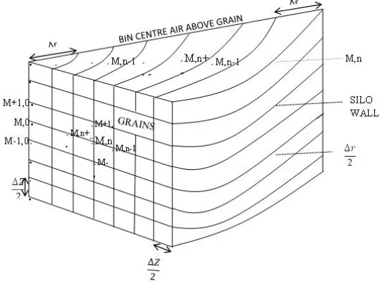
Mathematical model development. A section of the cylindrical grain metal silo was divided into a finite number of spatial elements in radial direc-tion, as shown in Fig. 2. The conductive heat trans-fer models, expressed in Poisson and Laplace

dif-ferential equations, were adopted and used as the guiding principle in this investigation.

2 q ₀ _{K T}

k

     _conduction

q

T q ThA

hA

    convection

Q = Ibv + Id radiation

Total heat transfer is therefore:

Q_t= KV2_{T + VT + h}

c2πrl(Ts –Tair) + Iblv + Id where: K – thermal conductivity; ∇T – temperature gradient in two dimensions; h_c– heat capacity (J·kg– 1_·K–1_);_r_{– base}

[image:3.595.66.376.101.285.2]

radius of the silo (m); l – height of the silo (m); T_s– inter-nal temperature of the silo (K); T_air – temperature of the surounding or outside air (K); s – Stefan-Boltzmann con-stant (5.6704 × 10–8_W·m–2_K–4_);_b_{– width of the silo (m)} Fig. 1. Cross section of the vertical silo type

Fig. 2. Finite element of spatial arrangement in grain metal silo

Temp/RH Probe

Loading hopper

19 m

11 m

Gate for uploading Ladder

Perforation for aeration

[image:3.595.69.344.551.756.2]

(4)

However, general differential equation of heat flow in two dimensions in a cylindrical system (Smithies et al. 1952; Carslow, Jaeger 1959) is given as:

2 2

δ _αδ 1 δ δ

δ δ δ δ

T T T T

t r r r y

 

 _  _

  (1)

T(ryt) = T_i (r,y) for t = 0

where: T_i – the initial grain temperature

Meanwhile, the heat transfer by conduction was computed using Eq. (3).

α ρ

g

p

K C



where: α – thermal diffusivity; K_g – thermal conductivity; ρ – bulk density; C_p – specific heat capacity; T – tem-perature of stored grains and is a function of independent variables of r and y at r–y plane; r, y – radial and vertical coordinates of the cylindrical storage silo; t – time

Now, considering the boundary conditions where the convective heat transfer coefficient and ambi-ent temperature exist in Fig. 2, the expression in Eq. (4) was used to compute the heat transfer in the silo due to convection.





δ δ ₀

δ δ

g T T c A

K h T T

r y

 

   

 

  (2)

The temperature at any point T_m_, which is dis-cretized in time. Subscript p was used to denote time dependence of T, and the time derivative is expressed in terms of the difference in tempera-tures associated with the new (p + 1) and previous (p) times. Hence calculations are performed at suc-cessive times separated by interval ∆t. The explicit form of finite difference of Eq. (2) for the interior mode m, n of the storage silo is:

1

, , 1, 1, ,

2

1, , , 1 , 1 ,

2 2 1

α

2 1

P P P P P

m n m n m n m n m n

P P P P P

m n m n m n m n m n

T T T T T

t r

T T T T T

m P r y



 

  

      

 

 _   



   

   

      

 _  _   _ 

   

   

(3)

Solving for the nodal temperature at the new (p + 1) time and assuming that ∆r = ∆y:

(4)

where: F₀ – finite-difference form of the Fourier number

2

α

o r

F r  



However, using L' Hospital’s rule Eq. (1) can be transformed into:

2

2 0

1 δ δ δ δ lim

r

T T

r r y



 _{ }

 

 

Therefore, Eq. (1) for the centre of the silo can be written as:

2 2

δ _α δ δ

δ δ δ

T T T

t r y

 

 _  _

  (5)

For centre of the silo, where r = 0 (m = 0, n = 0) at new time (p + 1) is:









1

0,0P

4

0 1,0P 0,1P 0, 1P

1 6

0,0P 0

T



F T

T

F









(6) In practice, the surface temperature changes with variation of the outside temperature. LO and CHEN (1986) reported that for point on outside surfaces which are exposed to convective condi-tions, the finite difference equation must be ob-tained by applying the energy balance method to a control volume about that node. As a result of this, the finite difference form of the Eq. (1) for the surface points with specified convective boundary condition at the new time (p + 1) is given as:









1 1

, 1, , 1 , 1

0 1

0 ,

2 2

1 1

2 1 4

1 1

P

P P P P a

m n m n m n m n

c w

P m n c w

B T

T F T T T

h L Kw F B

F T

h L Kw



  

 

 _    _



 

 

 

 _  _



 

  (7)

where: K_w – thermal conductivity of the silo wall (W· mK–1_);_L

w – thickness of the silo wall (m); TPa –

ambient temperature at time, p (°C); B₁– the finite-dif-ference form of the Biot number and is given as:

I c

g

h r B

K  

The finite element computer program was de-veloped to solve Eq. (7). The input data are the node and element, boundary condition, thermal properties of grain, air and storage material, initial temperature of every node in the domain, outside temperature and the thickness of the silo wall. The nodal temperature for the new time is determined exclusively by known nodal temperatures for the

, 0 1, 1, , 1 , 1

, 0

1 1

1

1 4

P P P P P

m n m n m n m n m n

P m n

T F T T T T

m

T F

m

   

   

 _ _  _   _

 

 

  

 _  _  __

 

(5)

previous time. In this way, the transient tempera-ture distribution was obtained by successively in-crementing t by ∆t. By repeating this procedure, the temperature distribution within the silo was computed.

Development and execution of simulation protocol

The deterioration of grains in metal silo is usu-ally associated with a lot of energy emissions in the form of temperature. This realisation was used as a basis for simulating the model developed in this investigation. Thus, in order to take care of sudden increases in temperature within the silo, the model was designed to predict temperature slightly high-er than both the measured and ambient temphigh-era- tempera-ture values. A flow diagram of the simplified ver-sion of the simulation protocol is shown in Fig. 3. The measured temperature data were used as

in-put data for the simulation exercise, which started during the rainy season and lasted for five months (May to September). Based on the input parameter controlling the fan operation, the grains boundary conditions were determined using forced convec-tion sub routines at the appropriate time interval. The finite element model expressed in Eq. (7) was thereafter used to predict the temperature from the centre and radii (3.25 and 8.25 m) of the metal silo.

RESULTS AND DISCUSSION

[image:5.595.72.324.89.474.2]

(6)

112

for predicting the temperature changes, from the months of May to September, were comparable with the ambient and measured values from the speci-fied radius (0, 3.25 m and 8.25 m) and at a depth of 1.2 m from the base of the silo (Figs 5 to 7). For both the centre and radii locations, the simulated temperatures followed the measured values more closely at 1.2 m depth. The model predicted that the temperatures at 1.2 m location increased from May through the end of September in comparison with the measured temperatures values. This may probably be associated with heat of respiration of the grains together with the accumulated heat gain during the day and long hours of sunshine. The var-iation occurring from July to the start of dry sea-son (September) might be responsible for the slight temperature build up in September.

It is also important to note that the pattern of temperature at the depth of 1.2 m from all the

[image:6.595.307.524.99.258.2]

specified radii of the silo did not differ from each other. For instance, the difference between the measured and ambient temperature from the cor-responding simulation value was less than 5°C, as is shown in Figs 6 and 7. This implies that the fi-nite element model can be relied upon for predict-ing the temperature variations within the storage silos and the interactive effects imposed by the ambient condition. In a related investigation, Al-abadan (2006) applied the finite difference model in 2-D, to predict the influence of bin diameter on the temperature variations within maize bulk stor-age. The author reported that the ambient tem-peratures during the dry season were higher than the wet season. Lawrence et al. (2013) also agreed with our findings, in their investigation on the ap-plication of 3-D transient heat, mass, momentum, and species transfer in the stored grain ecosystem, that grain surface temperature within the silo was Fig. 4. Validation of model for predicting silo temeprature

[image:6.595.77.272.100.255.2]

change at the centre and at a depth of 1.2 m Fig. 5. Validation of model for predicting silo temeprature change at depth of 1.2 m and radius of 3.25 m from centre

[image:6.595.80.276.577.725.2]

Fig. 7. Validation of model for predicting silo temeprature change at the centre and depth of 1.2 m

Fig. 6. Validation of model for predicting silo temeprature change at depth of 1.2 m and radius of 8.25 m from centre

!

0 5 10 15 20 25 30 35 M ay Ju

ne _July

A ug us t Se pt em be r Te m pe ra tu re (° C ) Storage period 0 5 10 15 20 25 30 35 40 M ay Ju

ne _July

A ug us t Se pt em be r Te m pe ra tu re (° C ) Storage period Ambient Simulated Measured 0 5 10 15 20 25 30 35 M ay Ju

ne _July

A ug us t Se pt em be r Te m pe ra tu re (° C ) Storage period 0 5 10 15 20 25 30 35 M ay Ju

ne _July

A ug us t Se pt em be r Te m pera tu re (° C ) Storage period 0 5 10 15 20 25 30 35 M ay Ju

ne _July

A ug us t Se pt em be r Te m pe ra tu re (° C ) Storage period Ambient Simulated Measured Ambient Simulated Measured Ambient Simulated Measured Ambient Simulated Measured Ambient Simulated Measured

!

0 5 10 15 20 25 30 35 M ay Ju

ne _July

!

0 5 10 15 20 25 30 35 M ay Ju

ne _July

!

0 5 10 15 20 25 30 35 M ay Ju

ne _July

[image:6.595.307.533.580.731.2]

(7)

Res. Agr. Eng. Vol. 64, 2018 (3): 107–114 https://doi.org/10.17221/101/2016-RAE

higher than the ambient by 5°C. Also, the research result of Lawrence and Maier (2012) was in line with our findings as the authors reported a differ-ence of 4°C between the different configurations of the cone used for maize storage.

Fig. 8 and Fig. 9 indicate that the temperature near the silo wall and at the 8.25 m was still higher than that in the bin centre and at 3.25 m when the ambient temperature began to rise in September. Should this not adequately and effectively be cor-rected during the period of storage, the high tem-perature incidence within the metal silo can cause the stored grains to spoil. The higher silo tempera-tures near the wall and at radius of 8.25 m might have been influenced by solar radiation between the silo roofing and surface layer. Thus, in order to avoid this from happening, vents are usually made through the silo walls or roof for the excess heat to escape (Laszlo and Adrian 2009). The research results of Zhang et al. (2016) corroborated our findings in their work on temperature variation in small grain steel silos. Furthermore, the varia-tion in the temperature within the metal silo can cause pressure build up in horizontal direction, just around the wall of the storage silo. In the view of Moran et al. (2012), the increment in the pres-sure developed is much experienced as variation in temperature increased. The implication of the pre-sent research results is that since there is no much difference between the measured and ambient air temperatures from the simulated, the overall effect can only result in lower pressure build up within the silo to such an extent that structural failure is not envisaged.

CONCLUSION

The temperature variation in the grain metal silo was investigated using finite element method (FEM). By taking temperature measurements at in-terval of 8 hours for 153 days from January to Sep-tember, a mathematical model was developed and used to simulate the temperature behaviour within the silo. The results of the simulation were com-pared with the ambient and measured values from specified radii (0, 3.25 m and 8.25 m) and at depth of 1.2 m from the base of the grain silo. The simu-lated results agree with the measured and ambient temperature data. The pattern of temperature at the depth of 1.2 m from the radii of the metal silo did not differ from each other. This may imply that the silo will need aeration at an interval of 8 hours to curtail excessive heat build-up that may lead to deterioration of stored grains and possible struc-tural failure.

References

Alabadan B.A. (2006): Temperature changes in bulk stored maize. AU Journal of Technology, 9: 187–192.

Casada M.E. (2000). Adapting a grain storage model in a 2-D generilised coordinate system. ASAE Annual International Meeting: 1–14.

Carslaw H.S., Jaeger J.C. (1959): Conduction of Heat in Solids. 2nd edition. Clarenden Press, Oxford.

[image:7.595.70.270.97.253.2]

David F.G. (1986): Dynamics of viscoelastic studies: a time domain finite element formulation. UTIAS report, No. 301. Institute for Aerospace studies, University of Toronto, XI. Fig. 8. Validation of model for predicting silo

[image:7.595.309.521.104.250.2]

teme-prature change of 1.2 m and radius of 3.25 m from the internal wall

Fig. 9. Validation of model for predicting silo temeprature change at a depth of 1.2 m and radius of 8.25 m from the internal wall

!

0 5 10 15 20 M ay Ju

ne _July

A ug us t Se pt em be r Te m pe ra tu re Storage period 0 5 10 15 20 25 M ay Ju

ne _July

A ug us t Se pt em be r Te m pe ra tu re (° Storage period Ambient Simulated Measured 0 5 10 15 20 25 30 35 M ay Ju

ne _July

!

0 5 10 15 20 25 M ay Ju

ne _July

A ug us t Se pt em be r Te m pe ra tu re (° Storage period 0 5 10 15 20 25 M ay Ju

ne _July

A ug us t Se pt em be r Te m pe ra tu re (° Storage period Ambient Simulated Measured 0 5 10 15 20 25 30 35 M ay Ju

ne _July

(8)

Jia C., Suna D. W., Caob C. (2001): Computer simulation of temperature changes in a wheat storage bin. Journal of Stored Products Research, 37: 165–177.

Laszlo R., Adrian T. (2009): Simulation of changes in a wheat storage bin regarding temperature, Analele Universităţii Din Oradea, Fascicula:Protecţia Mediului, 14: 239–244. Lawrence J., Maier D.E., Stroshine R.L. (2013):

Three-dimen-sional transient heat, mass, momentum, and species trans-fer in the stored grain ecosystem: Part II. Model validation. Transaction of the American Society of Agricultural and Biological Engineering, 56, 181–201.

Lawrence J., Maier D. E. (2012): Prediction of temperature distributions in peaked, Leveled and inverted cone grain mass configurations during aeration of corn. Applied En-gineering in Agriculture, American Society of Agricultural and Biological Engineers, 28: 685–692.

Lo K.M., Chen C.S. (1975): Simulation of temperature and moisture changes in wheat storage due to weather vari-ability. Journal of Agricultural Engineering Research, 20: 47–53.

Moran J. M., Aguado P. J., Ayuga F., Guaita M., Juan A. (2012): Effects of thermal loads on agricultural silos. In: 15th_ASCE

Engineering Mechanics Conference, June 2–5, Columbia University, New York: 1–8.

Sadhere R.C. (1993). Fundamentals of Engineering Heat and Mass Transfer. India, Wiley, Eastern Limited.

Yang W., Jia C.C., Siebenmorgen T. J., Howell T. A., Cnossen A. G. (2002): Intra–kernel moisture responses of rice to drying and tempering treatments by finite–element simula-tion. Transaction of the American Society of Agricultural and Biological Engineering, 45: 1037–1044.

Zhang L., Chen X., Liu H., Peng W., Zhang Z., Ren G. (2016): Experiment and simulation research of storage for small grain steel silo. International Journal Agricultural and Biological Engineering, 9: 170–178.