Scalable Engineering Calculations
on The Example of Two Component
Alloy Solidification
Elzbieta Gawronska, Robert Dyja, Andrzej Grosser, Piotr Jeruszka, Norbert Sczygiol
Abstract—Consideration of the issue of two-component alloy solidification with the usage of the finite element method may lead to the need to calculate the system of equations with millions of unknowns in which the coefficient matrix is the sparse matrix. In addition, symmetry of this matrix can be impaired with the introduction of boundary conditions. This sit-uation introduces laborious numerical calculations which - due of technical limitations – is practically impossible to speed up with the consideration of a single computational unit. Because of this reason, using parallel and distributed processing to resolve this issue becomes the interesting algorithmic problem. The paper focuses on the use of scalability of available development tools (libraries and interprocess communication mechanisms) to engineering simulation of two-component alloy solidification in the mold. An important aspect of the considerations are the ways parallelization of computations taking into account the fourth-type boundary condition – the contact between the two materials. The implementation uses a TalyFEM library. PETSc (Portable, Extensible Toolkit for Scientific Computation) library is the computing pillar of this set of classes and methods. It provides a programming interface which contains vectors, matrices, and solvers (including systems of linear equations) structures. This interface enables the automatic distributed data structures in a number of computational units using MPI (Message Passing Interface) whereby the communication itself is hidden from the programmer. This is an advantage during the desig of algorithms which use vectors and matrices. A problem solved with FEM can be parallelized in two ways: the parallelization on the mathematical formulas level (independent parts of the pattern can be calculated parallelly) and the division of tasks into smaller subtasks – assignment of nodes and elements into specific computational units. Such a division is called domain decomposition. The domain is a set of data on a single processor. Both methods can be used in the TalyFEM library, if the input files loading module is modified. We have designed our own parallel input module (finite element mesh) providing a division of loaded nodes and elements into individual computational units. These solutions enable the full potential of parallel computing available in the TalyFEM library using the MPI protocol. This implemented software can be run on any computer system with distributed memory.
Index Terms—parallel computing, distributed memory, FEM, solidification
I. INTRODUCTION
T
HE development of the computing power of personal computers increased the possibility of carrying out nu-merical calculations. Large engineering simulations, in which billion of unknown has to be estimated, can be calculated an ever shorter period of time on High Performance Comput-ing (HPC) systems. However, today’s PCs have sufficientlyManuscript received March 29, 2017; revised April 4, 2017.
E. Gawronska et al. are with the Faculty of Mechanical Engineering and Computer Science, Czestochowa University of Technology, Dabrowskiego 69, 42-201 Czestochowa, Poland, e-mail: [email protected]
powerful computational units which are able to solve small problems. Nowadays, due to technological limitations (size of the printed circuit boards can not be reduced indefinitely, disproportionate power in relation to the possibilities, etc.), the possibility of accelerating the calculations is focused on the use of multiple computational units in the same numeric process. Instead of accelerating the cycle frequency of one unit, a greater number of such units is used, especially on HPC systems. This also can be seen in today’s processors – they contain more cores but lack of a greater acceleration of the clock frequency.
Software needs to be adapted to such hardware. To effi-ciently utilize the possibilities of multi-core computing unit, the code must include parallel computation. In addition, the use of supercomputers, consisting of several thousands of nodes operating in parallel, requires scalable software project.
To avoid common problems in scalable software at the stage of designing the algorithms, distinguishment of ele-ments which can be calculated independently is required. Each portion that depends on the other requires the use of expensive and time-synchronization task to avoid errors resulting from the use of the same variables. This paper shows a method that uses separation of tasks into subtasks which can be calculated separately on each computing unit. The numerical method, which has been presented in this paper, uses a system of linear equations to calculate the results. Systems of equations usually stored in the form of a coefficients matrix and additional vectors are well described and implemented in the existing components and they are ready to be used in the source code. Vectors, matrices, and solvers – objects responsible for solving the system of equations – can operate parallelly, separating items into individual computational units. Our engineering software used ready-made data structure used to calculate the scalable systems of linear equations.
The presented issues such as: the division of tasks and parallel calculation of the unknown, had to be implemented in the form of packaged engineering software. From the soft-ware engineering’s viewpoint, this process can be accelerated by using the core of the finished application. The use of such core, adjusted it to the required applications, reduces the time needed for the design, creation and implementation of software.
the scientific problems connected with a system of equation obtained from the partial differential equations. Although, there are developed another methods, too, e.g. method of continuous source functions which is a boundary meshless method reducing the problem considerably comparing to other methods [3]. The rest of this article presents the numer-ical model, the use of preprocessor, the parallel methods of implementation of the model in the software, and the results.
II. SOLIDIFICATIONMODEL
Engineering calculations were performed on the example of the solidification process of an alloy. The model of solidification process is built on the basis of the equation of heat conduction with the source member [4]:
∇ ·(λ∇T) =cρ∂T ∂t −ρsL
∂fs
∂t (1)
wherein:T – temperaturet– time,λ– thermal conductivity,
c– specific heat,ρ– density,L– latent heat of solidification,
fs– the solid phase fraction.
A. Discretization of the Area and of the Time
Equation (1) is converted in the model using enthalpy for-mulation (basic capacitive forfor-mulation). As a result, it gives one equation that describes the liquid phase and the solid area of solidification. The apparent heat capacity formulation keeps the temperature as the unknown in the equation [5].
As a result of this transformation and the implementation of the discretization of the area by the finite element and the discretization of the time with the finite difference (Euler Backward modified scheme [6]), the linear system of equations was achieved. It has a suitable form to be solved by the one of the algorithms equations above:
(M+ ∆tK)Tt+1=MTt+ ∆tb (2) where:
K = Z
Ω
λ∇N∇NdΩ
M = Z
Ω
c∗(T)NNdΩ
b = Z
Γ
NλT,inidΓ
(3)
whereinK – the conductivity matrix,M– the mass matrix,
b– the boundary conditions vector,N– the shape function vector,i– spatial coordinates,Ω– the computational domain,
c∗ – effective heat capacity,Γ– boundary.
B. Boundary Conditions
The model uses two types of boundary conditions: the Newton’s boundary condition which models heat transfer be-tween volume and environment, and the boundary condition of contact, which reflects the flow of heat between the two domains (cast and mold) taking into account to the separation layer. Both of these boundary conditions are natural boundary conditions.
The introduction of the natural boundary conditions is carried out by means of elements which are the boundary’s
discretization. In the case of the three-dimensional mesh consisting of the tetrahedral elements, boundary elements are the triangular elements and introducing the boundary conditions is made with the following equations:
b1 b2 b3 = A 12
2 1 1 1 2 1 1 1 2
q1 q2 q3 (4)
This system is a solution of the integral in the expression definingbin the formula (Eq. 3), wherein Ais the area of the boundary element and q’s are the flows of heat at the boundary of a given vertex. The value of heat flux occurring in the formula is calculated in accordance with the type of boundary condition. For Newton’s boundary condition the following formula is used:
Γ : q=α(T−Tot) (5) whereinα– the coefficient of heat exchange with the envi-ronment,T – the temperature of the body on the boundaryΓ
andTot – the ambient temperature. In contrast, the following
formula shows the exchange of heat by the boundary layer separation:
Γ :
q=κ(T(1)−T(2)) T(1) 6=T(2)
(6)
wherein κ– a heat transfer of a separation layer, T(1) and
T(2) – the temperature of two areas on contact point. As it has been shown, the introduction of above boundary conditions requires modifying the coefficient matrix because the boundary conditions consist of a temperature of the current time step.
III. THEIMPLEMENTATION OF THEREQUIRED
FUNCTIONALITY
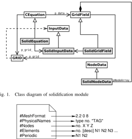
Implementation of the computing module using the TalyFEM library [7], [8] (with PETSc library, developed by [9]) requires the implementation of several classes, pre-sented in figure 1. The basic class is SolidEquation. It provides an implementation of assembling the global matrix and boundary conditions by means of overrid-denIntegrandsmethods andIntegrands4Side. An-other SolidInputData class manages loaded proper-ties of the material from the text file. The next class
SolidGridField, thanks to overriding theSetIC meth-ods with theGridFieldmethod, allows the initial condi-tions to be introduced. On the other hand,SolidNodeData
objects store the results in nodes. As noted in the in-troduction, one of the implementation problems was the inclusion of the boundary condition of the fourth type with the separation layer. To generate the Finite Element mesh, the GMSH preprocessor was used. That preprocessor allows entering many physical areas by setting appropriate flags for the material. This makes it possible to distinguish the cast, mold or external surfaces during the loading stage of the grid. TalyFEM was not compatible with files generated by the GMSH, therefore, implementation of several classes in order to load and distribute the parallel distribution of the data between all processes was required.
Fig. 1. Class diagram of solidification module
#MeshFormat #PhysicalNames #Nodes #Elements #Periodic
2.2 0 8 type no. "TAG" no. X Y Z
no. [desc] N1 N2 N3 ... N1 N2
Fig. 2. The*.mshfile data scheme.[desc]means a description of the
item which differs in syntax depending on the pre-processor and the element
elements with smaller dimension than the dimension of the task. For example, the boundary conditions of two-dimensional plates (divided into two-two-dimensional elements) refer to the one-dimensional edge which can be regarded as one-dimensional finite elements. Similarly, with a cube (three-dimensional finite elements) – boundary conditions apply to the two-dimensional walls. With the used library, all elements must be the same type which unfortunately, makes it difficult to use the data boundary (for example: to select only one surface element located on the edge of the area). This situation had to be resolved by the appropriate use of configuration data.
Another required functionality was to ensure proper oper-ation of the fourth boundary condition. In the solidificoper-ation model, the fourth condition requires a physical data derived from adjacent elements. For example, considering the heat transfer between the mold and the casting, the thermal conductivity of the two areas should have been taken into account. At the same time, it is apparent that the knowledge about the connections between nodes (a node of one area corresponding to the node of second area) is required.
A. Implementation of the GMSH Format
One of the essential elements of the simulation is to load input data representing the considered problem. The problem presented earlier loaded input data generated by the GMSH preprocessor. Due to the scalability of the TalyFEM library, the very process of loading must take into account the distribution of the data (nodes, elements) into processes. The figure 2 shows a diagram of the GMSH file. The implemen-tation of loading of this file needs to combine a declaration of physical conditions (here in the #PhysicalNames section) with the properties described in the simulation configuration file.
*.msh scheme format is simple. At the beginning, the
declarations of a physical object group – components of
a single type (eg. surface consisting of three walls) – are given. These objects combine some physical property. The GMSH preprocessor is not used to set specific value. It is only possible to select specific components to connect into a physical group. The next sections are a section of the nodes and the finite elements. The description of each node consists of a number of its current and subsequent coordinates. It should be noted that regardless of the dimension of the task, the GMSH saves the three-dimensional coordinates – the z coordinate is stored with a value of 0 for the two-dimensional tasks which had to be taken into account in implementation. The description of an element consists of the item index, a description of geometric and physical properties, and the serial indices of nodes that make up the item. A description of property, in the case of meshes generated for solidification, consists of four integers – the type of an element, unused value (usually a value of 2), the index of the physical object, and the geometry of the object. The type of an item and physical object of the group are important for the TalyFEM Library.
Loading nodes did not cause major implementation issues but loading elements required following a few rules. First of all, for the TalyFEM library, the main information about the physical properties (a boundary condition; they are called indicators in the library) are stored in objects representing nodes, and the .msh format stores this information in the elements. The library retains the image of a mesh consisting only of the elements of one type; GMSH also saves boundary elements. For the three-dimensional grid for calculations, tetrahedral elements should be only read; for boundary con-ditions, recorded triangular elements located on the surfaces of volume must be analysed. Loading nodes and elements can be divided into the following steps:
• load the number of nodes and move the position of the next character into the elements section;
• load the total number of elements and analyse the element. The loading module analyses the boundary elements and the space, creating a map of the node index of the physical property. After this step, the number of spatial elements is known, and this number determines the number of all the items used in the calculations; • load spatial elements;
• go back to nodes section and load nodes data using in-formation of the constructed map of physical properties of nodes.
The last interesting piece of the file is the information about nodes adjacent to each other (Periodic section)1 [10].
Basi-cally, this section consists of indices pairs, which represent nodes having the same coordinates. This information is used during the boundary condition of the fourth type with the contact of two boundaries.
The loading was implemented for two scenarios for the program based on TalyFEM:
• the calculation with the decomposition of the area (the grid division into smaller sub-areas stored on each process) which required the implementation of data communications;
1There are many mechanical and technological problems with the periodic
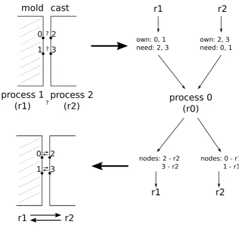
Fig. 3. Scheme of loading and decomposing data by the main process (process 0)
Fig. 4. The diagram of aggregation of data received from the main process
• calculation without decomposition of the area; all data is stored in one process only.
The first scenario is interesting from the programming point of view. The library supports parallel data storage with dis-tributed memory but low-level data, such as node coordinates or description of the elements, which had to be sent using the MPI interface [11]. Figure 3 shows a scheme of loading the.mshfile using decomposition area for the main process. The main process (process 0) reads information but does not keep it – the individual data is transferred to the separate processes. At the beginning, physical properties are loaded and broadcasted to all processes. It has been recognized that there is no need for the division of information into the individual processes. Such information requires very little memory resources compared with information about the mesh.
Then the analysis and loading of elements, including map of the physical properties of nodes is carried out. At this stage, information is sent in the form of a NxM matrix whereN is the number of elements for then-th process, and
M is the number of data describing an element – physically (for simplicity of communication) it is an array ofNxM size. Similarly, the information about the nodes is sent, wherein, additional information about physical group is transmitted (the physical properties of a given node) and information on the adjacent node (if the node does not have a boundary condition of the fourth kind, a value of −1 is sent). The task of the remaining processes is to take the data and assemble it in a simple dynamic arrays, what is presented in figure 4. The TalyFEM library converts information from the arrays into its object-oriented counterpart. There is no need for manual communications between different processes nor even involve other processes in the process of sending the data – excluding the information on the connected areas.
B. The Adjacent Nodes in Different Processes
[image:4.595.49.290.50.164.2]The problem with parallel processing of the fourth condi-tion mode arises due to the necessity of modifying a local matrix (in each process) using the physical parameters and a
Fig. 5. The scheme of exchanging information on adjacent nodes (in the boundary condition of the fourth type)
local matrix of neightbouring element. To properly assemble the system of equations, the knowledge of a pair of nodes that have the same coordinates (but belong to different areas) is required. These nodes can belong to different processes. Moreover, one process does not have information on the location (process rank) of its adjacent node. As shown in figure 5, communication during the loading of the mesh is limited to the communication of the main process with other processes. Another difficulty is the renumbering nodes while performing of the parMETIS tools – the numbers of nodes from a .msh file are converted to the numbers optimal in parallel communication. Each process keeps the map of the physical index of the node (specified in the
.msh file) in solution index but this map is limited solely to the ones stored in the process. The library and the modifications (shown in the next section) require knowledge about the number of nearly processes (contain neighbouring nodes). To avoid troublesome point-to-point (peer-to-peer) communication, the data repository seeking for all adjacent nodes was used in the 0 process.
Any process obtaining the nodes and converting them into an object, analyses the proximity of the node. As shown in the previous section, information about a node consists of coordinates, the index of physical groups, and the index (according to the numbering of the preprocessor) of adjacent node. For process 0, the following information is prepared:
• map of the index from .msh file into the solution index of nodes which are adjacent to another node (and, therefore, they will be adjacent to the another node); • the physical indices of those nodes for which
informa-tion about the process is required.
[image:4.595.50.287.197.272.2]Fig. 6. The relevant area. Cast has dark gray color, mold – light gray
value is provided by TalyFEM so there is no need for manual communications between processes.
Above solution is not scalable (parallelization is not used to speed up calculations), but is necessary for the proper im-plementation of the fourth-type boundary condition. Further, the finding of adjacent nodes is executed only once, while loading task properties.
IV. RESULTS
Performance tests were done on the CyEnce computer lo-cated at Iowa State University. CyEnce is a cluster consisting of 248 computing nodes each with two eight-core Intel Xeon E5 and 128 GB RAM. The calculations were made for the area shown in the figure 6.
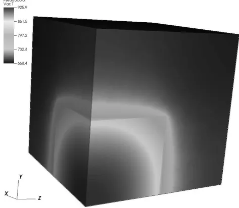
This area consists of a cast (dark gray) and mold (light gray). As shown, the mold is a cube with a side of 0.2 , m. The cast also has the shape of a cube but with a side of0.1m. The Al2Cu alloy is the material for the cast; steel – for the mold. The heat exchange between the cast and the mold was held using the boundary condition of 4th type including the separation layer. A thermal conductivity of the release layer was equal to1000W/m2K. Heat transfer through the mold to the environment was held with the boundary condition of the third type in which the heat transfer coefficient was equal to10W/mK. The initial cast temperature is equal to960K; mold – 660 K. Exemplary distributions of temperature for different time instants are shown in the figures 7, 8, 9. The results are consistent with the physics of the phenomenon.
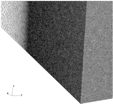
Performance tests were made for two sizes of finite ele-ments mesh: small (of 3.5 million eleele-ments, see Fig. 10), and big (of 25 million elements, see Fig. 11). The time required to perform 100 steps of simulation (where the size of the time step was equal to 0.05 s) is shown in the charts on figures 12 and 13.
[image:5.595.52.285.52.246.2]For performance testing, the output file saving has been switched off because the analysed times and the preaparation of the calculation could be affected by the writing operation. The charts show summarised loading time of retrieve data from files operation and the operations described in Chapter III. The initialization time is the time to perform optimal decomposition of the area into the sub-areas. The number
Fig. 7. Temperatures in the relevant area after 5 s
Fig. 8. Temperatures in the relevant area after 25 s
[image:5.595.307.542.289.496.2] [image:5.595.306.543.529.735.2]Fig. 10. Mesh details with 3.5 milion elelemnts
[image:6.595.311.540.55.227.2]Fig. 11. Mesh details with 25 milion elelemnts
Fig. 12. Time required to perform 100 steps of simulation in mesh with 3.5 million elements
of sub-areas was equal to the number of processors used. The calculation time consists of assembling the system of equations and subsequent solution. The GMRES method was used to solve the system of equations [12].
V. CONCLUSIONS
[image:6.595.78.260.248.414.2]The paper presents the use of libraries that support calcu-lations which use the finite element method applied to the solidification simulation. Although the TalyFEM library had
Fig. 13. Time required to perform 100 steps of simulation in mesh with 25 million elements
already been tested on computers of high power, its use in solving a specific problem required adding essential pieces of code. The essence of the research presented in the paper was to answer the question of how changes affect the performance and to determine the ability of using computers of distributed memory for calculations.
The results show that despite the limitations of the in-put/output operations, the example performs efficiently for large tasks and it provides good scalability while the load time equals the time of calculation.
REFERENCES
[1] O. C. Zienkiewicz and R. L. Taylor,The finite element method; 5th ed. Oxford: Butterworth, 2000.
[2] N. Sczygiol,Modelowanie numeryczne zjawisk termomechanicznych w krzepncym odlewie i formie odlewniczej. Politechnika Czstochowska (in Polish), 2000.
[3] V. Kompiˇs and Z. Murˇcinkov´a, “Thermal properties of short fibre composites modeled by meshless method,” Advances in Materials Science and Engineering, vol. 2014, p. 521030, 2014.
[4] J. Mendakiewicz, “Identification of solidification process parameters,” Computer Assisted Mechanics and Engineering Sciences, vol. Vol. 17, no. 1, pp. 59–73, 2010.
[5] R. Dyja, E. Gawronska, A. Grosser, P. Jeruszka, and N. Sczygiol, “Estimate the impact of different heat capacity approximation methods on the numerical results during computer simulation of solidification,” Engineering Letters, vol. 24, no. 2, pp. 237–245, 2016.
[6] W. L. Wood,Practical time-stepping schemes / W.L. Wood. Clarendon Press ; Oxford University Press Oxford [England] : New York, 1990. [7] H.-K. Kodali and B. Ganapathysubramanian, “A computational frame-work to investigate charge transport in heterogeneous organic pho-tovoltaic devices,” Computer Methods in Applied Mechanics and Engineering, vol. 247-248, pp. 113–129, 2012.
[8] O. Wodo and B. Ganapathysubramanian, “Computationally efficient solution to the cahnhilliard equation: Adaptive implicit time schemes, mesh sensitivity analysis and the 3d isoperimetric problem,”Journal of Computational Physics, vol. 230, no. 15, pp. 6037–6060, 2011. [9] S. Balay, W. D. Gropp, L. C. McInnes, and B. F. Smith, PETSc
2.0 User Manual, Argonne National Laboratory, 2014. [Online]. Available: http://www.mcs.anl.gov/petsc/
[10] S. Legutko, K. Zak, and J. Kudlacek, “Characteristics of geometric structure of the surface after grinding,”MATEC Web Conf., vol. 94, p. 02007, 2017. [Online]. Available: https://doi.org/10.1051/matecconf/ 20179402007
[11] University of Tennessee, Knoxville. (2016) MPI: A message passing interface. [Online]. Available: http://mpi-forum.org/docs/ mpi-3.0/mpi30-report.pdf
[image:6.595.55.282.449.619.2]