A Novel MAC Protocol for Improving the
Throughput in Multi-Hop Wireless Networks
Takumi Sanada, Xuejun Tian, Takashi Okuda, and Shi Xiao,
Abstract—WLANs have become increasingly popular and widely deployed. The MAC protocol is one of the important technology of the WLANs and affects communication efficiency directly. In this paper, focusing on MAC protocol, we propose a novel protocol that network nodes dynamically optimize their backoff process to achieve high throughput in multi-hop wireless networks. Distributed model MAC protocol has an ad-vantage that no infrastructure such as access point is necessary. On the other hand, total throughput decreases heavily under a high traffic load due to the hidden node problem, which needs to be improved. Through theoretical analysis, we find that the average idle interval per a node can represent current network traffic load and can be used together with estimated number of neighbor nodes for setting optimalCW. Through simulation comparison with a conventional method and recently a proposed method, we show that our scheme can greatly enhance the throughput in saturated case.
Index Terms—WLANs, multi-hop, MAC, backoff, throughput
I. INTRODUCTION
W
IRELESS Wireless local area networks (WLANs) have become increasingly popular and widely de-ployed. In two channel access methods DCF (Distributed Coordination Function) and an optional centralized PCF (Point Coordination Function), due to inherent simplicity and flexibility, the DCF is preferred in the case of no base station such as vehicle to vehicle communications. Since all the nodes share a common wireless channel with limited bandwidth in the WLANs, it is highly desirable that an efficient and fair medium access control (MAC) scheme is employed. In multi-hop wireless networks, the transmission range of a node is not large enough to transmit to every nodes in the entire network area. In that case, the transmission between two nodes may require more than one hop. Thus, the throughput decreases rapidly due to the hidden node problem. Several researches have been proposed in [1], [2], [3], [4], [5], [6], [7] for alleviating the hidden node problem. In [1], [2], [3], [4], the multi-channel MAC protocol was proposed. In [1], the authors proposed a MAC protocol, which employs two radio interfaces per node. One interface follows fast hopping and is mainly for transmission, while the other interface follows slow hopping and is generally for reception. The works in [3], [4] adopt the busy tone to deliver the data packets successfully. The other nodes that hear the busy tone should suspend their attempts for data transmissions. In [6], the authors proposed the multiple receiver transmissionTakumi Sanada is with School of Information Science and Technology, Aichi Prefectural University(email: [email protected])
Xuejun Tian is with School of Information Science and Technology, Aichi Prefectural University(email: [email protected])
Takashi Okuda is with School of Information Science and Technology, Aichi Prefectural University(email: [email protected])
Shi Xiao is with school of Electronic and Electrical Engineering, Wuhan textile University(email:[email protected])
(MRT), the fast NAV (Network Allocation Vector) truncation (FNT) and the adaptive receiver transmission (ART) shceme. For alleviating the receiver blocking problem, each node transmits to multiple receivers in MRT scheme and the NAV duration in RTS packet reduces in FNT protocol. Considering the drawbacks from the MRT and FNT schemes, the ART scheme further improves the throughput.
The above most works are used in limited network and not flexible enough. For example, the works in [3], [4] assume that each network node needs to use at least two transceivers, which is merely utilized in wireless networks. The MRT and ART schemes in [6] assume that each node has multiple destination nodes. Also, most works do not take the backoff process into account to improve the throughput. In multi-hop wireless networks, the collisions are caused by the neighbor nodes or the hidden nodes, which is more than single hop wireless networks. Thus, for improving the throughput, the optimal backoff process is required to avoid the collisions. In [8], authors proposed a novel MAC protocol by observing the channel to estimate the number of nodes and tuning the network to obtain high throughput with good fairness according to the number of nodes. This is proved to be effective but assumes that the network is in single-hop wireless networks. In this paper, for expanding the work [8] in multi-hop wireless networks, we propose a novel MAC protocol that dynamically optimizes each node’s backoff process for multi-hop wireless networks. We call it OBM. The models on throughput analysis have been investigated in [9], [10], [11], [12] for multi-hop wireless networks. These models is refered in the performance analysis of proposed OBM.
The remainder of this paper is organized as follows. In Section II, we elaborate on our key idea and the theoretical analysis for improvement. Then, we present in detail our proposed OBM scheme. Section III gives performance eval-uation and the discussions on the simulation results. Finally, concluding remarks are given in Section IV
II. ANALYSIS AND THEPROPOSAL OFOPTIMIZING
BACKOFF BYDYNAMICALLYESTIMATINGNUMBER OF
NEIGHBORNODES
In the IEEE 802.11 MAC, an appropriateCW (Contention Window) is the key to providing throughput. In multi-hop wireless networks, the collisions are caused by the neighbor nodes or the hidden nodes, which is more than single hop. Thus, network nodes need to obtain the optimalCWin order to avoid the collisions. In OBM, By observing the channel, all nodes adjust the optimal CW and we can obtain high throughput.
In this analysis, we have the following assumptions: • For simplicity, the transmission, interference and
• Each node uses the RTS/CTS exchange and contends for the medium with the same probability p, where
p denotes the transmission probability at a randomly chosen chosen time slot.
• All nodes always have packets to transmit.
A. Optimal Backoff
The analytical model is derived based on the standpoint of a tagged node. In a given time slot, there are three states in a tagged node, that is, the idle state, the successful transmission state, and the collision state. In the idle state, the tagged node counts down its backoff timer during the channel is idle. Otherwise, its backoff timer is freezed due to either the physical or virtual carrier sensing mechanisms because the neighbor node of the tagged node transmits a packet. In the successful transmisison state, after the backoff timer has reached zero, the tagged node transmits RTS and DATA packets successfully. In the collision state, the tagged node fails to transmit the RTS packet due to collision caused by either the neighbor nodes or the hidden nodes of the tagged node. By calculating the probabilities of these states, the throughput of the tagged node can be obtained. In the following, we give the probabilities that the tagged node is in the idle state, the successful transmission state and the collision state, respectively.
The tagged node in the idle state means that the tagged node does not transmit RTS or DATA packets, the probability that the tagged node is in the idle state is denoted byPidl, it can be expressed as
Pidl= 1−p. (1)
There are three cases if the tagged node is in the idle state as follows: Case 1: All nodes within the carrier sensing range of the tagged node do not transmit any packets; Case 2: Only one node within the carrier sensing range of the tagged node transmits packets; Case 3: Two or more nodes within the carrier sensing range of the tagged node transmit packets. We denote byPidl 1,Pidl 2, andPidl 3the probabilities of the three cases, respectively. Thus, we can express the above probabilities as
Pidl 1 = (1−p)n
Pidl 2 = (1−p)(n−1)p(1−p)n−2
Pidl 3 = Pidl−Pidl 1−Pidl 2 (2)
wherenis the average number of neighbor nodes including the tagged node, that is, the average number of nodes within the tagged node’s carrier sensing range. The tagged node in Case 1 remains for the duration of a slot timetslt. We denote by Tidl 2 andTidl 3 the time duration of Case 2 and Case 3, respectively. These time durations can be expressed as
Tidl 2 = TRT S+TCT S+TDAT A+TACK
+4τ+ 3SIF S+DIF S
Tidl 3 = TRT S+τ+EIF S (3)
whereTRT S,TCT S,TDAT AandTACK are the transmission duration for a RTS packet, a CTS packet, a DATA packet and a ACK packet, respectively. τ is the maximum propagation delay between two nodes.
For simplicity, we assume that the transmission is success-ful when a RTS packet is transmitted successsuccess-fully. In fact, a DATA packet may be collided due to transmissions of the hidden nodes. This case is caused due to large interference range as shown in [13]. In this analysis, for simplicity, we assume that DATA packet is not collided. Therefore, the transmission of the tagged node is successful when the neighbor nodes of the tagged node do not transmit packets in the same time slot and the hidden nodes of that do not transmit during the vulnerable period ηRT S, which can be calculated asηRT S =⌈(TRT S+TSIF S)/Tslot⌉. We denote byPsthe probability that the tagged node is in the successful transmission state, which can be expressed as
Ps=p(1−p)n−1(1−p)2ηRT SH(r) (4)
where r is the distance between the transmitter and the receiver.H(r)is the number of hidden nodes of the tagged node and depends onr. We denote byTtx the time duration for successful transmission, which equalsTidl 2.
Moreover, we denote by Pcol the probability that the tagged node is in the collision state. The tagged node is in the collision state in the case that the tagged node transmits a RTS packet and a collision is caused by neighbor nodes or hidden nodes. The probability that the tagged node is in the collision state is expressed as
Pcol = p{1−(1−p)n−1}
+p(1−p)n−1{1−(1−p)2ηRT SH(r)}
= p−p(1−p)n−1(1−p)2ηRT SH(r) (5)
We denote by Tcol the time duration for collision, which equalsTidl 3.
Consequently, using the above probabilities of three states, the throughput per a node is expressed as
ρ = {LPs}/{tsltPidl 1+Tidl 2Pidl 2
+Tidl 3Pidl 3+TtxPs+TcolPcol} (6) where L is the total number of bits in the payload. Our aim is to maximize the throughput shown in Eq.(6). To this end, we need to obtain the optimal CW according to the network condition such as the number of neighbor nodes. In the following, we give the method for estimating the number of neighbor nodes on line by three parametersPidl 1,Pidl 2 andPidl 3which can be obtained directly by listening to the channel for a certain interval. Then, using obtained Pidl 1,
Pidl 2 andPidl 3, we give the method for maximizing the throughput dynamically. Calculating the number of neighbor nodes directly by Eq.(2) is inefficient and unrealistic. Here, we use a simple and effective method which is suitable for real time estimating. With Eqs.(1) and (2), we obtain
Pidl 1=Pidln . (7)
Letfidl(n) =Pidln , wherePidl, i.e.,Pidl 1,Pidl 2andPidl 3 are known parameters andn is the unknown parameter that needs to be estimated. We find thatfidl(n)is the monotone function. We take the derivative offidl(n)with respect ton, and let dndf ={log(1−p)}(1−p)n. It can be found that df
dn is not plus whenpchanges from 0 to 1.
0 0.1 0.2 0.3 0.4 0.5 0.6 0.7 0.8
30 35 40 45 50 55 60 65 70
fidl
(n)
Number of Neighbor Nodes
Pidl_1=0.605(p=0.01)
Pidl_1=0.077(p=0.05)
fidl(n) (p=0.01)
[image:3.595.308.542.55.221.2]fidl(n) (p=0.05)
Fig. 1. Monotone functionfidl(n)when the real value ofnis 50
decreases as the number of neighbor nodes is increasing. SincePidl 1 is a known value,fidl(n)should be adjusted in agreement with Pidl 1. When Pidl 1 is equal to fidl(n), n is the number of neighbor nodes deployed in real network.
The above characteristic is favorable for estimating the number of neighbor nodesnwhich can be calculated by the following dichotomy. Supposing n is in a range [0, nmax], initially let ntry1 = nmax/2 and substitute it into fidl(n). Then compare fidl(ntry1) with Pidl 1. If fidl(ntry1) >
Pidl 1, we should setntry2= [ntry1+nmax]/2. Otherwise, we should set ntry2 = [ntry1+ 0]/2 for the following cal-culation. Obviously, this method is simple and effective. For example, when nmax= 100, we just need to calculate four times to estimatenin the worst case with maximum error 3. In the following, we present the condition of high throughput. And then, we give the method of how to dynamically tune
CW to enhance throughput. The average idle slot interval is denoted by Lidl, it can be expressed as
Lidl=
Pidl
1−Pidl
. (8)
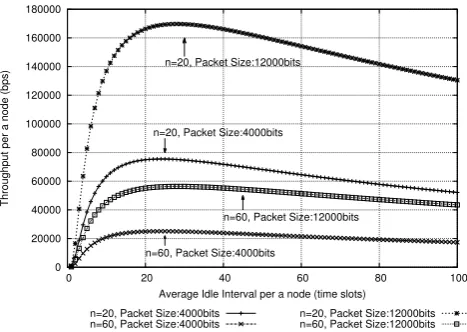
With Eqs.(6) and (8), thinking IEEE 802.11b, we can express the throughput per a node as a function ofLidl/nwith SIFS = 10s, DIFS = 50s, ACK = 304bits and slot time = 20s, as shown in Fig. 2.PsandPcolare concerned with the distance
r between the transmitter and the receiver. We assume that the transmission range is 250m and we set asr= 125in Fig. 2. From the figure, first, we find that every curve follows the same pattern; namely, as the average idle slot interval per a node Lidl/n increases, the throughput first rises quickly, and then decreases relatively slowly after reaching its peak. Second, although the optimal value ofLidl/nthat maximizes throughput is different in cases of different frame lengths or number of neighbor nodes, it varies in a very small range. Therefore, Lidl/n is a suitable measure that indicates the network throughput and we can obtain the following equation
Lidl/n=α. (9)
As shown in Fig. 2, considering the different frame lengths and number of neighbor nodes, we can set asα= 25. From Eqs.(1) and (8), we havep= 1/(Lidl+1), thenp= 1/(nα+
1)with Eq.(9). SubstitutepinPidl 1= (1−p)n, it becomes
0 20000 40000 60000 80000 100000 120000 140000 160000 180000
0 20 40 60 80 100
Throughput per a node (bps)
Average Idle Interval per a node (time slots) n=20, Packet Size:4000bits
n=20, Packet Size:12000bits
n=60, Packet Size:4000bits
n=60, Packet Size:12000bits
n=20, Packet Size:4000bits
[image:3.595.49.285.56.222.2]n=60, Packet Size:4000bits n=20, Packet Size:12000bitsn=60, Packet Size:12000bits
Fig. 2. Throughput with average idle slot interval per a node
as following,
opt Pidl 1= (1−
1
nα+ 1)
n (10)
whereopt Pidl 1 is the optimal Pidl 1 that maximizes the throughput. From the Eq.(10), according to the number of neighbor nodes, each node can calculate the opt Pidl 1, that is, set the optimalCW to obtain the high throughput. Each node can observe the current Pidl 1. (denoted by
cur Pidl 1.) By Comparingcur Pidl 1withopt Pidl 1, the
tagged node adjusts the CW to obtain the optimal CW as following,
IF(cur Pidl 1·µ1≤opt Pidl 1)
CW ←CW·λ1(⇒Increase)
IF(cur Pidl 1·µ2≤opt Pidl 1< cur Pidl 1·µ1)
CW ←CW·λ2(⇒Increase)
IF(cur Pidl 1·µ3≤opt Pidl 1< cur Pidl 1·µ2)
CW ←CW
IF(cur Pidl 1·µ4≤opt Pidl 1< cur Pidl 1·µ3)
CW ←CW·λ3(⇒Decrease)
IF(opt Pidl 1< cur Pidl 1·µ4)
CW ←CW·λ4(⇒Decrease).
(11)
We set empirical datas µ1 = 1.05, µ2 = 1.025, µ3 = 0.99 andµ4= 0.95to determine the different densities ofPidl 1. Also, λ1 = 1.5, λ2 = 1.1, λ3 = 0.9 and λ4 = 0.5 are empirical datas to adjust the increasing or decreasing changes of CW. Since we are interested in tuning the network to obtain maximal throughput, given the Eq.(11), we can achieve this goal by adjusting the size of CW. In other words, each node can estimate the number of neighbor nodes and adjust its backoff window accordingly so that the throughput of the tagged node is maximized.
B. OBM Scheme
As mentioned above, we can obtain the optimal CW by Eq.(11) by using the estimated number of active neighbor nodes. Hence, each node can adjust its CW dynamically and tune the network to deliver high throughput. To obtain the Pidl and Pidl 1, we can count the number of backoff slots (denoted byCidl 1) and RTS transmissions of neighbor nodes (denoted by Cidl 2 3). To avoid occasional cases,
the counters when a certain number of RTS transmissions reaches a certain number γ. The Pidl and Pidl 1 can be calculated as
Pidl =
Cidl 1+Cidl 2 3
Cidl 1+Cidl 2 3+γ
Pidl 1 =
Cidl 1
Cidl 1+Cidl 2 3+γ
. (12)
The tagged node calculates theCW before packet transmis-sions. After newCW (denoted by newCW) is obtained, the
CW can be updated as
CW =β·CW+ (1−β)·newCW (13)
whereβ is a smoothing factor with the range of [0,1]. The higher β leads to stability but maybe reduces adaptivity to network changes such as in traffic and active nodes.
However we assume that all nodes have the number of neighbor nodes, in the actual network, all nodes do not have the same number of neighbor nodes and the same informations of the channel. The corner nodes which deploys in the corner of the network have smaller number of neighbor nodes than the center nodes which deploys in the center of the network have. Consequently, the corner nodes have more chances to transmit RTS packet and smallerCW than center nodes have. For keeping balance between the corner nodes and the center nodes, the corner nodes have almost the same CW as the center nodes have. After adjusting the CW as shown in Eq.(11), theCW of the corner nodes adjust as CW =CW·λ1, where λ1= 1.5 is an empirical data. Before adjusting theCW again, theCW of the corner nodes adjust as CW = CW/λ1. In OBM, we adds the value of estimated the number of neighbor nodes in RTS packet to distinguish the corner node from the center node. The tagged node receives any RTS packets and obtains the average number of neighbor nodes which is calculated by the estimated number of neighbor nodes that the neighbor nodes have. Then, the tagged node is determined as the corner node when the estimated number of neighbor nodes of the tagged node is smaller than half of the average number of neighbor nodes. Otherwise, the tagged node is determined as the center node.
In the following, we give the tuning algorithm.
1) The tagged node begins listening to a channel and countsCidl 1 andCidl 2 3 individually.
2) When the tagged node needs backoff and the number of RTS transmissions reaches a certain number γ, it calculates the optimalCW as a new CW and resets
CW according to Eq.(13). If the tagged node is corner node, the CW of that is adjusted for resetting CW
before calculating the optimalCW.
3) By comparing the estimated number of neighbor nodes with the average number of neighbor nodes, the tagged node is determined as the corner node or the center node.
4) If the tagged node is the corner node, theCW of that is adjusted for keeping balance between the corner nodes and the center nodes.
5) It resets counting Cidl 1 andCidl 2 3
The certain number of RTS transmissions γ needs to be set appropriately. When theγis small,CW changes rapidly with network changes. In contrast, if the γ is large, the network
TABLE I
NETWORK CONFIGURATION
Parameter Value
SIFS 10µsecs
Slot time 20µsecs
EIFS 364µsecs
DIFS 50µsecs
MinCW∼MaxCW 31∼1023 Max retry threshold 7
Buffer size 256000 bits
Data rate 11Mbps
transmission range 250m carrier sensing range 550m Path loss exponent 4
can have higher stability but is short of adaptivity. In the following simulation, we set as γ = 2. As shown in [14], the maximal throughput is not obtained when all nodes have the sameCW. In OBM, each node adjusts theCW around the optimal value according to cur Pidl 1 and opt Pidl 1. Using this method, high throughput is achieved, which can be found in the following simulations.
III. PERFORMANCEEVALUATION
In this section, we evaluate the performance of our OBM through simulations, which are carried out on OPNET Mod-eler [15]. For comparison purpose, we also present the simulation results for the IEEE 802.11b DCF and the FNT scheme in [6]. In [6], the authors proposed the MRT, the FNT and the ART scheme. The MRT and the ART scheme assume that each node has multiple destination nodes. We focus on the unicast mode and compare OBM with the FNT scheme. In the FNT scheme, the NAV duration in RTS packet reduces fromTCT S+TDAT A+TACK+3SIF StoSIF S+TCT S+τ in order to alleviate the receiver blocking problem. The simulation parameters are shown in TABLE I and the OBM-specific parameters in TABLE II. In the conventional method, sets the maximum CW but in OBM, there is no upper bound ofCW. In analysis, we assume that the transmission, interference and sensing ranges of all network nodes are the same value. The simulations are carried out in a realistic setting, that is, the transmission and sensing rages are about 250m, 550m, respectively. We assume that network nodes are distributed at random within an area of 3000 × 3000
m2 as shown in Fig. 3. We considere the only nodes that are deployed in the center of the network in order to avoid the effect of the corner nodes. To maintain the required density, the network is divided into nine areas. The nodes are distributed at random in each area. Each node selects another node at random as a receiver and generates traffics according to a Poisson process with the same arrival rate. The arrival rates are high enough to achieve the saturated network. The packet size is 8000 bits, which is the size of payload data at MAC layer and does not include MAC overhead. As shown below, OBM exhibits a better performance.
A. Estimated number of neighbor nodes
TABLE II
BACKOFF PARAMETERS
Parameter Value
Maximum number of neighbor nodes 100
α 25
β 0.8
γ 2
0 1000 Length [m]
2000
1000 2000 3000
[image:5.595.55.288.60.388.2]Width [m] 3000
Fig. 3. A snapshot of node distribution in simulations when average number of neighbor nodes is 20
that the estimated number of neighbor nodes changes to inappropriate value because of the beginning of simulation and then converges to a comparatively stable value around 50 after about 20s, which is related to algorithm of backoff parameters shown in TABLE II. Also, the estimated number of neighbor nodes that the corner nodes have is smaller than the estimated number of neighbor nodes that the center nodes have. Thus, OBM can estimate the number of neighbor nodes dynamically and distinguish the corner nodes from the center nodes.
0 10 20 30 40 50 60 70
0 10 20 30 40 50
Estimated Number of Neighbor Nodes
Simulation time [sec]
center node 1, 2
corner node 1, 2 center node 1
[image:5.595.51.283.584.748.2]center node 2 corner node 1 corner node 2
Fig. 4. Estimated number of neighbor nodes with simulation time when average number of neighbor nodes is 50
0 2000 4000 6000 8000 10000 12000
20 25 30 35 40 45 50 55 60
Average Throughput per a node [bps]
Number of Neighbor Nodes OBM
FNT
DCF
DCF FNT OBM
Fig. 5. Throughput with neibor node numbers
B. Throughput
Second, we give the throughputs of three schemes, i.e., OBM, IEEE 802.11b DCF and FNT in [6]. Fig. 3 shows the results of the average throughput per a node with a different number of neighbor nodes. The throughput is the only value of payload data successfully received and does not include other pakcets.
The throughputs of three shcemes decrease with the aver-age number of neighbor nodes increasing because the number of hidden nodes increases. In DCF and FNT schemes, the hidden node problem has a significant influence. These schemes applies an binary exponential backoff algorithm which takes time for obtaining theCW around the optimal value. This is the mainly reason that many collisions and the sharp decrease of the throughput. The FNT scheme obtains higher throughput than DCF when the number of neighbor nodes is 20. In FNT, the NAV duration in RTS packet reduces and increase the transmission probability. Thus, the collision probability increases when the number of neighbor nodes is large. The throughput of FNT is improved when the number of neighbor nodes is small, however, the throughput of that is almost the same as DCF when the number of neighbor nodes is larger than 20. The FNT scheme does not alleviate the effect of the hidden node problem enough. In contrast, OBM alleviates the effect of the hidden node problem and obtain high throughput. The maximum improvement of throughput is about 2 times when the number of neighbor nodes is 40.
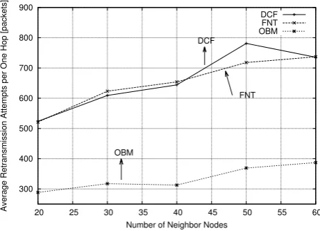
C. Retransmission attempts
300 400 500 600 700 800 900
20 25 30 35 40 45 50 55 60
Average Retransmission Attempts per One Hop [packets]
Number of Neighbor Nodes OBM
DCF
[image:6.595.51.282.55.222.2]FNT DCF FNT OBM
Fig. 6. Retransmission attempts with neibor node numbers
However, these ranges are not the same value in this sim-ulation. As shown in simulation results, OBM can adopt in that case.
IV. CONCLUSION
In this paper, we proposed a novel MAC protocol OBM that enhance DCF in multi-hop wireless networks. In OBM, each node observes Pidl 1, Pidl 2 and Pidl 3 to estimate the number of neighbor nodes and then sets CW around the optimal value dynamically according to the number of neighbor nodes. Thus, OBM can obtain high throughput. From analysis and simulation results, this scheme is effective and can adjust the network change promptly. Moreover, OBM can alleviate the hidden node problem and achieve higher throughput than IEEE 802.11 DCF and recently a proposed method. Compared to recently proposed methods, OBM is flexible enough. In OBM, the RTS packet is added few bits in order to distinguish the corner node from the center node, however, the multiple transceivers, channels or destination nodes are not used. As a future work, we need verify by actual environment and evaluate the validity of OBM.
REFERENCES
[1] K. H. Almotairi and X. S. Shen, “A distributed multi-channel MAC protocol for ad hoc wireless networks,” IEEE Trans. Mob. Comput., vol. 14, no. 1, pp. 1–13, 2015. [Online]. Available: http://doi.ieeecomputersociety.org/10.1109/TMC.2014.2316822 [2] K.-P. Shih, Y.-D. Chen, and S.-S. Liu, “A collision avoidance
multi-channel mac protocol with physical carrier sensing for mobile ad hoc networks,” inAdvanced Information Networking and Applications Workshops (WAINA), 2010 IEEE 24th International Conference on, April 2010, pp. 656–661.
[3] H. Zhai, J. Wang, and Y. Fang, “Ducha: A new dual-channel mac protocol for multihop ad hoc networks,” Trans. Wireless. Comm., vol. 5, no. 11, pp. 3224–3233, Nov. 2006. [Online]. Available: http://dx.doi.org/10.1109/TWC.2006.04869
[4] T. Ito, K. Asahi, H. Suzuki, and A. Watanabe, “Researches and evaluation of strong busy tone that improves the performance of ad-hoc networks,” inMobile Computing and Ubiquitous Networking (ICMU), 2014 Seventh International Conference on, Jan 2014, pp. 182–187. [5] X. Yao and Y. Wakahara, “Application of synchronized multi-hop
protocol to time-variable multi-rate and multi-hop wireless network,” inNetwork Operations and Management Symposium (APNOMS), 2013 15th Asia-Pacific, Sept 2013, pp. 1–6.
[6] K.-T. Feng, J.-S. Lin, and W.-N. Lei, “Design and analysis of adap-tive receiver transmission protocols for receiver blocking problem in wireless ad hoc networks,”IEEE Transactions on Mobile Computing, vol. 12, no. 8, pp. 1651–1668, 2013.
[7] H. Zhai and Y. Fang, “A solution to hidden terminal problem over a single channel in wireless ad hoc networks,” inMilitary Communica-tions Conference, 2006. MILCOM 2006. IEEE, Oct 2006, pp. 1–7. [8] X. Tian, T. Sanada, T. Okuda, and T. Ideguchi, “A novel mac protocol
of wireless lan with high throughput and fairness,” in 38th Annual IEEE Conference on Local Computer Networks, 2013, pp. 688–691. [9] A. A. Abdullah, F. Gebali, and L. Cai, “Modeling the
throughput and delay in wireless multihop ad hoc networks,” in Proceedings of the 28th IEEE Conference on Global Telecommunications, ser. GLOBECOM’09. Piscataway, NJ, USA: IEEE Press, 2009, pp. 5711–5716. [Online]. Available: http://dl.acm.org/citation.cfm?id=1811982.1812327
[10] Y. Wang, N. Yan, and T. Li, “Throughput analysis of ieee 802.11 in multi-hop ad hoc networks,” inWireless Communications, Networking and Mobile Computing, 2006. WiCOM 2006.International Conference on, Sept 2006, pp. 1–4.
[11] Y. Gao, D.-M. Chiu, and J. C. Lui, “Determining the end-to-end throughput capacity in multi-hop networks: Methodology and applications,” SIGMETRICS Perform. Eval. Rev., vol. 34, no. 1, pp. 39–50, Jun. 2006. [Online]. Available: http://doi.acm.org/10.1145/1140103.1140284
[12] P. Li and Y. Fang, “Saturation throughput of ieee 802.11 dcf in multi-hop ad hoc networks,” inMilitary Communications Conference, 2008. MILCOM 2008. IEEE, Nov 2008, pp. 1–7.
[13] K. Xu, M. Gerla, and S. Bae, “How effective is the ieee 802.11 rts/cts handshake in ad hoc networks,” inGlobal Telecommunications Conference, 2002. GLOBECOM ’02. IEEE, vol. 1, Nov 2002, pp. 72– 76 vol.1.
[14] X. TIAN, X. CHEN, T. IDEGUCHI, and Y. FANG, “Improving throughput and fairness in wlans through dynamically optimizing backoff(wireless communication technologies),” IEICE transactions on communications, vol. 88, no. 11, pp. 4328–4338, nov 2005. [Online]. Available: http://ci.nii.ac.jp/naid/110004019577/