Integrated Supply Chain Inventory Model with Progressive Carbon Taxation

(1)

Abstract—Mitigating carbon emissions is a considerable issue in the global supply chain nowadays. This paper presents an integrated inventory model with progressive carbon taxation which minimizes total cost and carbon emissions. Results analysis of the numerical example indicate that excess progressive cost of the second gap and transport lot significant impact on the integrated inventory policy.

Index Terms—Integrated inventory, progressive carbon taxation, supply chain

I. INTRODUCTION

Facing global warming and climate change, the government and enterprise effort to reduce carbon emissions. The United Nations, the European Union and many governments have enacted legislations or designed mechanisms such as carbon taxes, carbon offset, clean development, cap and trade, carbon caps and joint implementation to curb the total amount of carbon emissios [1]. Firms develops a series of reforms and connects a green supply chain. They are undertaking initiatives to reduce their carbon footprints in response to mechanisms or legislations, expectation of customer and environmental responsibility.

Greenhouse Gases, which is the culprit of global warming and climate change, includes carbon dioxide (CO2), methane (CH4), nitrous oxide (N2O), Chlorofluorocarbons (CFCs) and sulfur hexafluoride (SF6). According to the investigation of Intergovernmental Panel on Climate Change (IPCC) found that carbon dioxide causes the greenhouse effect occupied the highest proportion. Further, the amount of carbon dioxide emissions is related to the carbon content of fuels. As a result, many countries achieve carbon reduction targets with carbon taxes.

Carbon taxes is a kind of price policy, and is calculated based on carbon-containing of the general common energy which such as oil, coal, electricity and natural gas. Carbon tariff achieve rational allocation of environmental costs, internalizing the externality cost and also known as Pigovian

Ming-Feng Yang is with Department of Transportation Science, National Taiwan Ocean University, No.2, Beining Rd., Jhongjheng District, Keelung City 202, Taiwan, R.O.C. (phone: +886-2-24622192#7011; fax:+886-2-24633745; e-mail: yang60429@mail.ntou.edu.tw)

Yan-Ying Zou is with Department of Transportation Science, National Taiwan Ocean University, No.2, Beining Rd., Jhongjheng District, Keelung City 202, Taiwan, R.O.C. (e-mail: k41229@gmail.com.)

Ming-Cheng Lo (Corresponding Author) is with Department of Business Administration, Chien Hsin University of Science and Technology, No.229, Jianxing Rd., Zhongli City, Taoyuan County 32097, Taiwan, R.O.C. (e-mail: lmc@uch.edu.tw)

Yen-Ting Chao is with Department of Information Management, Taipei Chengshih University of Science and Technology, No. 2, Xueyuan Rd., Beitou, 112 Taipei, Taiwan, R.O.C. (e-mail: ytchou@tpcu.edu.tw)

taxes. For industry, carbon taxes is a persistent and clear price signals. Corporations can conduct financial plan in accordance with the tax rates, and invest equipment or technology for reduce carbon emissions. A well-designed carbon tax system has double dividend. The first dividend is restrain carbon emission. The second dividend, the government has the carbon tax revenue which can reduce the levy to other taxable items (the income tax) or inject research and development in low-carbon technology as well as social welfare spending. Carbon taxes have the effect of tax circulation; hence, carbon taxes possess revenue neutral feature [2].

Chen et al. [3] note that firms have focused for the most part on reducing emissions through innovations of the physical processes involved, for example by redesigning products and packaging, deployment and use of less polluting sources of energy, or replacing energy in efficient equipment and facilities. Bonney and Jaber [4] found out increasing the amount of products transported and reducing the frequency of delivery compared to those proposed by the traditional EOQ model gives better results in terms of ordering costs and carbon emissions. Benjaafar et al. [5] showed that how important insights could be drawn by integrating carbon emissions parameters into traditional and widely used lot-sizing models.

However currently firms put more emphasis productivity and customer satisfaction, which leads firms to focus on their supply chain and integrated logistics [6]. Yang et al. [7] developed a model which is useful particularly for integrated inventory systems where the vendor and the buyer form a strategic alliance for profit sharing. El Saadany et al. [8] studied a simple two-echelon supply chain model in which demand depends on the environmental quality of the systems(measured using 30 criteria) and the associated costs. Wahab et al. [9] offer an approach to optimally define the delivery/production policy to minimize the total cost of supply in a global supply chain.

Ghosh and Shah [10] examine some supply chain coordination with players initiating product “greening”. Cooperation between stakeholders does lead to higher greening levels but also to higher retail prices. In some coordination cases, the retailer has to provide suitable incentives to the manufacturer for him to participate in the bargaining process [11]. Swami and Shash [12] develop a model with a manufacturer and a retailer that coordinate their operations(wholesale price and green effort for the manufacturer, market price and green effort for the retailer). They propose a two-part tariff contract to produce channel coordination and „greener‟ efforts.Further, Chiu et al. [13] suggest the fuzzy multi-objective integrated logistics model with the transportation cost and demand fuzziness to solve

Integrated Supply Chain Inventory Model with

Progressive Carbon Taxation

(2)

green supply chain problems in the uncertain environment. Teck-Koon [2] presented four EOQ inventory management models, respectively the carbon tax, carbon emissions permissions, progressive taxation and regressive taxation.

The purpose of this research is develop a novel model that takes into account the link between inventory policy, carbon taxes and green supply chain. The construction of model is based on EOQ model with progressive carbon taxation [2] and integrated inventory model [14]; then to minimize both the total costs and carbon emissions.

This paper is organized as follows. Section II defined the parameters and assumptions. Next, Section III develops the integrated inventory model with carbon taxes. After that, Section IV solved the model to get the optimal solution and showed numerical examples in Section V. Finally, this leads over the discussion of the findings and future research opportunities.

II. NOTATIONS AND ASSUMPTIONS

In order to develop an integrated inventory model with progressive carbon tax, this research adopted progressive carbon tax. Progressive carbon tax is a levy in a tax system where the tax rate increases as the taxable base (carbon emission) increases. Excess progressive rate is determined by the excess part of carbon emissions as the progressive basis. The following notations and assumptions below are used to build the model:

A. Notations

To establish the mathematical model, the following notations and assumptions are used.

Q=order quantity of the purchaser, a decision variable Q*= the optimal order quantity

m= an integer representing the number of lots in which the items are delivered from the vendor to the purchaser, a decision variable

m*= the optimal transport lots

y= the first gap ceiling of excess progressive rate

β1= excess progressive tariff of the first gap per unit carbon

emission

β2= excess progressive tariff of the second gap per unit

carbon emission

r = annual inventory holding cost per dollar invested in stocks

Purchaser side

D = average annual demand per unit time A = purchaser‟s ordering cost per order L = length of lead time

Cp=purchaser‟s purchasing cost per unit

e0 = carbon emissions of empty trucks generate by

purchaser

e = variable carbon emissions factor per transport unit g0 = fixed carbon emissions of holding inventory generate

by purchaser

g = variable carbon emissions factor per holding unit 𝐶𝑂₂𝑝= carbon emissions of the purchaser

TECp= purchaser‟s total expected annual cost

Vendor side

P =vendor‟s production rate

S= vendor‟s set-up cost per set-up Cv=vendor‟s purchasing cost per unit

f0= carbon emissions of empty trucks generate by vendor

f = variable carbon emissions factor per transport unit h0= fixed carbon emissions of holding inventory generate

by vendor

h = variable carbon emissions factor per holding unit 𝐶𝑂₂𝑣= carbon emissions of the vendor

TECv = vendor‟s total expected annual cost

JTEC* = the optimal values of the expected joint total cost JTECi = the expected joint total cost, i = 1, 2, 3, 4*

*“i” represents four different cases

𝐶𝑠𝑠𝑒 1 ∶ 𝐶𝑂2

𝑝_{𝑄 > 𝑦, 𝐶𝑂} 2𝑣 𝑄 > 𝑦 𝐶𝑠𝑠𝑒 2 ∶ 𝐶𝑂2

𝑝

𝑄 > 𝑦, 𝐶𝑂2𝑣 𝑄 ≤ 𝑦 𝐶𝑠𝑠𝑒 3 ∶ 𝐶𝑂2

𝑝

𝑄 ≤ 𝑦, 𝐶𝑂2𝑣 𝑄 > 𝑦 𝐶𝑠𝑠𝑒 4 ∶ 𝐶𝑂2

𝑝

𝑄 ≤ 𝑦, 𝐶𝑂2𝑣 𝑄 ≤ 𝑦

B. Assumptions

(i) This supply chain system consists of a single vendor and a single purchaser for a single product.

(ii) The product is manufactured with a finite production rate P, and P > D.

(iii) The government divided the carbon emissions into two gaps, the first gap ceiling is y, and β1 < β2.

(iv) The demand X during lead time L follows a normal distribution with mean 𝜇_𝐿and standard deviation σ 𝐿. (v) The reorder point (ROP) equals the sum of the expected demand during lead time and the safety stock.

(vi) Shortages are not allowed.

(vii) Inventory is continuously reviewed

III. MODEL FORMULATION

In this section, we discuss the model of purchaser and vendor combined them into an integrated inventory model with progressive carbon tax.

A. The purchaser’s total expected cost

Based on the above notations and assumptions, the total expected annual cost for the purchaser 𝑇𝐸𝐶𝑝 = Ordering cost +

Holding cost + Carbon tax cost.

To start with, since A is the ordering cost per order, the expected ordering cost per year is given by:

(i) Ordering cost = 𝐷 𝑄 𝐴

From assumption (v), the reorder point ROP = μL + kσ 𝐿𝑖𝑗, where k is known as the safety factor. Then, the average on-hand inventory for the purchaser is shown as 𝐼 P≅

𝑄 2+

𝑅𝑂𝑃 − 𝜇𝐿= 𝑄

2+ kσ 𝐿.Hence, (ii) Holding cost = r𝐶𝑝(

𝑄

2+ kσ 𝐿)

After that, carbon tax cost is calculated with carbon emission of transportation and warehousing, as external costs of production to reflect environmental costs. The carbon emission of the purchaser is presented as

𝐶𝑂₂𝑝(𝑄) = 𝑒0+ 𝑒𝑄

𝐷

𝑄+ 𝑔0+ 𝑔 𝑄 2 =

𝑒0𝐷

𝑄 + 𝑔𝑄

2 + 𝑒𝐷 + 𝑔0(1).

(3)

(iii) Carbon tax cost = y𝛽₁+ (𝑒0𝐷

𝑄 + 𝑔𝑄

2 + 𝑒𝐷 + 𝑔0− 𝑦)𝛽2

.

If 𝐶𝑂₂𝑝 𝑄 ≤ 𝑦,

(iv) Carbon tax cost = (𝑒0𝐷

𝑄 + 𝑔𝑄

2 + 𝑒𝐷 + 𝑔0)𝛽1.

B. The vendor’s total expected cost

For the vendor‟s inventory model, its total expected annual cost 𝑇𝐸𝐶𝑣= set − up cost + Holding cost + Carbon tax cost.

First, because S is the vendor‟s set-up cost per set-up, and the production quantity for the vendor in a lot will be mQ, and (i) Set-up cost =(𝐷

𝑚𝑄)S.

Second, the vendor produces the item in the quantity of mQ, and the purchaser would receive it in m lots, with which each having a quantity of Q. For the vendor, its average inventory can be evaluated as follows: (see Fig I.)

𝐼 _𝑣= 𝑚𝑄 𝑄

𝑃+ 𝑚 − 1

𝑄 𝐷 −

𝑚2𝑄2

2𝑃 −

𝑄

𝐷 1 + 2 + ⋯ +

𝑚 − 1 𝑄 /(𝑚𝑄

𝐷) = 𝑄

2 𝑚 1 −

𝐷

𝑃 − 1 +

2𝐷

𝑃 , and therefore

(ii) Holding cost = r𝐶_𝑣 𝑄

2 𝑚 1 −

𝐷

𝑃 − 1 +

2𝐷 𝑃

Next, the carbon emission of the vendor is represented as

𝐶𝑂₂𝑣_{(𝑄) = 𝑓}

0+ 𝑓𝑄

𝐷

𝑚𝑄+ 𝑕0+ 𝑕 𝑄 2 =

𝑓0𝐷

𝑚𝑄+ 𝑕𝑄

2 + 𝑓𝐷

𝑚 + 𝑕0 (2). However, if 𝐶𝑂₂𝑣_{𝑄 > 𝑦}

(iii) Carbon tax cost = y𝛽₁+ (𝑓0𝐷

𝑚𝑄+ 𝑕𝑄

2 + 𝑓𝐷

𝑚 + 𝑕0− 𝑦)𝛽2

.

If 𝐶𝑂₂𝑣_{𝑄 ≤ 𝑦}

(iv) Carbon tax cost = (𝑓0𝐷

𝑚𝑄+ 𝑕𝑄

2 + 𝑓𝐷

𝑚 + 𝑕0)𝛽1.

Q

quantity

time Q/P

quantity

time mQ

mQ/P

Q/D Accumulated inventory for

vendor

[image:3.595.40.287.321.725.2]

Accumulated inventory for purchaser mQ/D

Fig 1. The inventory pattern for the vendor [14]

C. The expected joint total cost

According to the four different conditions, the expected joint total cost function, 𝐽𝑇𝐸𝐶_𝑖 𝑄, 𝑚 = 𝑇𝐸𝐶_𝑝+ 𝑇𝐸𝐶_𝑣 can be expressed as

𝐽𝑇𝐸𝐶𝑖(𝑄, 𝑚) =

𝐽𝑇𝐸𝐶1 𝑄1, 𝑚1 𝑓𝑜𝑟 𝐶𝑠𝑠𝑒 1

𝐽𝑇𝐸𝐶3(𝑄3, 𝑚3) 𝑓𝑜𝑟 𝐶𝑠𝑠𝑒 3

where

𝐽𝑇𝐸𝐶1 𝑄, 𝑚 =𝐷_𝑄 𝐴 +_𝑚𝑆 + 𝛽2(𝑒0+_𝑚𝑓0) +𝑄₂ 𝑟 𝑚 1 −𝐷_𝑃 −

1 +2𝐷

𝑃 𝐶𝑣+ 𝐶𝑝 + 𝛽2(𝑔 + 𝑕) + 𝛽2 𝐷 𝑒 + 𝑓

𝑚 + 𝑔0+ 𝑕0 +

2𝑦 𝛽1− 𝛽2 + 𝑟𝐶𝑝𝑘𝜎 𝐿 (3)

𝐽𝑇𝐸𝐶2 𝑄, 𝑚 =𝐷_𝑄 𝐴 +_𝑚𝑆 + 𝑒0𝛽2+𝑓0_𝑚𝛽1 +𝑄₂ 𝑟 𝑚 1 −𝐷_𝑃 −

1 +2𝐷

𝑃 𝐶𝑣+ 𝐶𝑝 + 𝑔𝛽2+ 𝑕𝛽1 + 𝛽1 𝑓𝐷

𝑚 + 𝑕0+ 𝑦 + 𝛽2 𝑒𝐷 +

𝑔0− 𝑦 + 𝑟𝐶𝑝𝑘𝜎 𝐿 (4)

𝐽𝑇𝐸𝐶3 𝑄, 𝑚 =𝐷_𝑄 𝐴 +_𝑚𝑆 + 𝑒0𝛽1+𝑓0_𝑚𝛽2) +𝑄₂ 𝑟 𝑚 1 −𝐷_𝑃 −

1 +2𝐷

𝑃 𝐶𝑣+ 𝐶𝑝 + 𝑔𝛽1+ 𝑕𝛽2 + 𝛽1 𝑒𝐷 + 𝑔0+ 𝑦 + 𝛽2 𝑓𝐷

𝑚 +

𝑕0− 𝑦 + 𝑟𝐶𝑝𝑘𝜎 𝐿 (5)

𝐽𝑇𝐸𝐶4 𝑄, 𝑚 =𝐷_𝑄 𝐴 +_𝑚𝑆 + 𝛽1(𝑒0+_𝑚𝑓0) +𝑄₂ 𝑟 𝑚 1 −𝐷_𝑃 −

1 +2𝐷

𝑃 𝐶𝑣+ 𝐶𝑝 + 𝛽1(𝑔 + 𝑕) + 𝛽1 𝐷 𝑒 + 𝑓

𝑚 + 𝑔0+ 𝑕0 +

𝑟𝐶𝑝𝑘𝜎 𝐿 (6) To minimize 𝐽𝑇𝐸𝐶_𝑖 𝑄, 𝑚 , this paper set ∂𝐽𝑇𝐸𝐶𝑖 𝑄𝑖,𝑚𝑖

𝜕𝑄_𝑖 = 0

and obtain the value of Q = 𝑄₁∗_{, 𝑄}

2∗, 𝑄3∗ 𝑎𝑛𝑑 𝑄4∗.

𝑄1∗=

2𝐷 𝐴+_𝑚𝑆+𝛽2(𝑒0+𝑓0_𝑚)

𝑟 𝑚 1−𝐷_𝑃 − 1+2𝐷_𝑃 𝐶𝑣+𝐶𝑝 +𝛽2(𝑔+𝑕)

0.5

(7)

𝑄₂∗₌ 2𝐷 𝐴+

𝑆

𝑚+𝑒0𝛽2+𝑓0𝛽 1𝑚

𝑟 𝑚 1−𝐷_𝑃 − 1+2𝐷_𝑃 𝐶𝑣+𝐶𝑝 +𝑔𝛽2+𝑕𝛽1

0.5

(8)

𝑄₃∗₌ 2𝐷 𝐴+

𝑆

𝑚+𝑒0𝛽1+𝑓0𝛽 2𝑚

𝑟 𝑚 1−𝐷_𝑃 − 1+2𝐷_𝑃 𝐶𝑣+𝐶𝑝 +𝑔𝛽1+𝑕𝛽2

0.5

(9)

𝑄4∗=

2𝐷 𝐴+_𝑚𝑆+𝛽1(𝑒0+𝑓0_𝑚)

𝑟 𝑚 1−𝐷_𝑃 − 1+2𝐷_𝑃 𝐶𝑣+𝐶𝑝 +𝛽1(𝑔+𝑕)

0.5

(10)

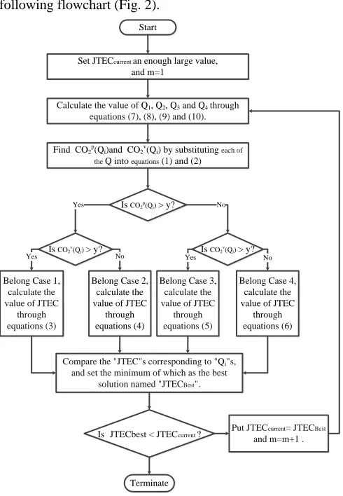
IV. SOLUTION PROCEDURE

Summarizing the above arguments, we establish the following algorithm to obtain the optimal values of 𝑄∗_,_𝑚∗

and 𝐽𝑇𝐸𝐶∗_{, where}_{the other parameters are known.} Algorithm

Step 1. Set m =1 and substitute into (7), (8), (9) and (10) to obtain Q1, Q2, Q3 and Q4, ∀i = 1, 2, 3, and 4.

Step 2. Find 𝐶𝑂₂𝑝 𝑄𝑖 𝑎𝑛𝑑 𝐶𝑂2𝑣 𝑄𝑖 by substituting Qi into (1)

and (2), ∀i = 1, 2, 3, and 4.

Step 3. Compare between 𝐶𝑂₂𝑝 𝑄𝑖 , 𝐶𝑂2𝑣 𝑄𝑖 , 𝑎𝑛𝑑 𝑦.

According to the different conditions, calculate corresponding JTECi using (3), (4), (5) or (6). ∀i = 1, 2, 3, and 4.

(4)

(Qi, m) < JTECi (Qi, m +1). ∀i = 1, 2, 3, and 4.

Step 5. The optimal 𝑚∗_{= 𝑚; 𝑄}∗_{= 𝑄}

𝑖, 𝑎𝑛𝑑 𝐽𝑇𝐸𝐶∗ 𝑄∗, 𝑚∗

= 𝐽𝑇𝐸𝐶𝑖(𝑄𝑖, 𝑚𝑖) , ∀i = 1, 2, 3, and 4. CO2v

The solution procedure of the whole system is shown in the following flowchart (Fig. 2).

Start

Calculate the value of Q1, Q2, Q3 and Q4through equations (7), (8), (9) and (10).

Find CO2p(Qi)and CO2v(Qi) by substituting each of theQ into equations (1) and (2)

Is CO2p(Qi) > y?

Yes No

Is CO2v(Qi) > y?

Belong Case 2, calculate the value of JTEC

through equations (4)

No

Yes

No

Yes

Compare the "JTEC"s corresponding to "Qi"s, and set the minimum of which as the best

solution named "JTECBest".

Is JTECbest < JTECcurrent? Put JTEC_{and m=m+1 .}current= JTECBest

Set JTECcurrent an enough large value,

and m=1

[image:4.595.36.281.131.485.2]

Terminate

Fig 2. Flowchart of the solution procedure

V. NUMERICAL EXAMPLE

To illustrate the proposed solution procedure, consider an inventory item with parameters tabulated in Table I.

Table I. Parameters of the example

Applying the equation and algorithm already given in this article, the optimal integer policy is shown in Table II.

Table II. The optimal solution for given parameters

The findings of the numerical result indicated that the minimum cost is $2,090 and carbon emission is 1138 tons with the optimal order quantity is 136 and transport lot is 4 in the integrated chain.

VI. CONCLUSION

With the pressure of global warming and climate change recently, reducing carbon emission has been becoming a trend of supply chain management. In this research, we formulated integrated inventory model with progressive carbon taxation. Both order quantity and transport lot are important factor to impact the inventory policy. Furthermore, excess progressive cost of the second gap which play significant role impact the optimal order quantity.

The numerical results showed that progressive carbon taxation is useful curb the carbon emission for integrated inventory systems because the purchaser and vendor made an effort to decrease carbon emission which remains in the vicinity of the standard. However, progressive carbon taxation also obstructs mass production.

REFERENCE

[1] A. Choudhary, S. Sarkar, S. Settur, M.K. Tiwari. “A carbon market sensitive optimization model for integrated forward–reverse logistics” International Journal of Production

Economics, Vol. 164, pp. 433–444, 2015.

[2] T-K, Ng. “Development and Analysis of Inventory Management Model Considering Carbon Tax”, Transportation and Logistics Management Department, National Chiao Tung University. 2012.

[3] X. Chen, S. Benjaafar, A. Elomri, “The carbon-constrained EOQ”, Operations Research Letters, Vol. 41, pp. 172–179, 2013.

[4] M. Bonney, M. Y. Jaber. “ Environmentally responsible inventory models: non-classical models for a non-classical era”

International Journal of Production Economic, Vol. 133(1), pp.

43–53, 2011.

[5] S. Benjaafar, Y. Li, M. Daskin. “ Carbon footprint and the management of supply chains: insights from simple models”

IEEE Transactions on Automation Science and Engineering,

Vol. 10(1), pp. 99–116, 2013.

[6] M.S. Pishvaee, F. Jolai, J.A. Razmi, “Stochastic optimization model for integrated forward/ reverse logistic network design”,

Journal of Manufacturing Systems, Vol. 28, pp.107–114. 2009.

common purchaser vendor

m ≦ 7 D 1000 P 3200

R = 0.2 A 25 S 400

L = 42 Cp 25 Cv 20

K = 2.33 Carbon emission parameters

σ = 7 e0 65 f0 180

y = 500 e 0.02 f 0.01

β1 = 0.06 g0 40 h0 110

β2 = 0.1 g 1.4 h 0.9

m Qi Q* CO2p CO2v CO2T JTEC*

1 Q3 373 495 770 1266 2503

2 228 505 612 1117 2195

3 Q1 169 563 545 1108 2111

4 136 633 505 1138 2090

5 114 709 479 1188 2095

6 Q2 100 783 458 1241 2113

[image:4.595.304.562.132.278.2]

(5)

[7] M.-F. Yang, M.- C. Lo, T. -P. Lu. “ A vendor-buyers integrated inventory model involving quality improvement investment in a supply chain”, Journal of Marine Science and Technology, Vol. 21 (5), pp. 586-593, 2013.

[8] El Saadany, A.M.A., M.Y. Jaber, M. Bonney. “ Environmental performance measures for supply chains”, Management

Research News, Vol. 34(11), pp. 1202–1221, 2011.

[9] M.I.M. Wahab, S.M.H Mamun, P. Ongkunaruk. “EOQ models for a coordinated two-level international supply chain considering imperfect items and environmental impact”

International Journal of Production Economic, Vol. 134(1), pp.

151–158, 2011.

[10] D. Ghosh, J. Shah, “A comparative analysis of greening policies across supply chain structures”, International Journal of

Production Economics, Vol. 135(2), pp. 568–583, 2012.

[11] H. Vincent, B. Laurent, “The carbon-constrained EOQ model with carbon emission dependent demand”, International Journal

of Production Economics, Vol. 164, pp. 285-291, 2015.

[12] S.Swami, J.Shash,”Channel coordination in green supply chain management”, Journal of the Operational Research Society, Vol. 64, pp. 336–351, 2013.

[13] C.Y. Chiu, Y. Lin, M.F. Yang. “Applying Fuzzy Multi-objective Integrated Logistics Model to Green Supply Chain Problems”

Journal of Applied Mathematics, Vol. 2014, ID 767095, 12

pages, 2014.

[14] JCH Pan, J.S. Yang. “A study of an integrated inventory with controllable lead time” International Journal of Production