Proceedings of the 2012 Student Research Workshop, pages 13–18,
Active Learning with Transfer Learning
Chunyong Luo, Yangsheng Ji, Xinyu Dai, Jiajun Chen State Key Laboratory for Novel Software Technology,
Department of Computer Science and Technology, Nanjing University, Nanjing, 210046, China {luocy,jiys,daixy,chenjj}@nlp.nju.edu.cn
Abstract
In sentiment classification, unlabeled user reviews are often free to collect for new products, while sentiment labels are rare. In this case, active learning is often applied to build a high-quality classifier with as small amount of labeled instances as possible. However, when the labeled instances are insufficient, the performance of active learning is limited. In this paper, we aim at enhancing active learning by employing the labeled reviews from a different but related (source) domain. We propose a framework Active Vector Rotation (AVR), which adaptively utilizes the source domain data in the active learning procedure. Thus, AVR gets benefits from source domain when it is helpful, and avoids the negative affects when it is harmful. Extensive experiments on toy data and review texts show our success, compared with other state-of-the-art active learning approaches, as well as approaches with domain adaptation.
1 Introduction
To get a good generalization in traditional supervised learning, we need sufficient labeled instances in training, which are drawn from the same distribution as testing instances. When there are plenty of unlabeled instances but labels are insufficient and expensive to obtain, active learning (Settles, 2009) selects a small set of critical instances from target domain to be labeled, but costs are incurred for each label. On the other hand, transfer learning (Ji et al., 2011), also known as domain adaptation (Blitzer et al., 2006), aims at
leveraging instances from other related source domains to construct high-quality models in the target domain. For example, we may employ labeled user reviews of similar products, to predict sentiment labels of new product reviews. When the distributions of source and target domain are similar, transfer learning would work well. But significant distribution divergence might cause negative transfer (Rosenstein et al., 2005).
To further reduce the labeling cost and avoid negative transfer, we propose a framework, namely Active Vector Rotation (AVR), which takes advantage of both active learning and transfer learning techniques. Basically, AVR makes model’s parameter vector actively rotate towards its optimal direction with as few labeled instances in target domain as possible. Specifically, AVR first applies certain unsupervised learning techniques to make source and target domain’s distributions more ‘similar’, and then leverages source domain information to query the most informative instances of target domain. Most importantly, it carefully reweights instances to mitigate the risk of negative transfer. AVR is general enough to incorporate various active learning and transfer learning modules, as well as varied basic learners such as LR and SVM.
2 Related Work
Shi et al. (2008) proposed an approach AcTraK, using labeled source and target domain instances to build a so-called ‘transfer classifier’ to help label actively selected target domain instances. AcTraK initially requires labeled target domain instances,
and relies too much on the transfer classifier. Thus it might be degenerated by negative transfer.
An ALDA framework was proposed in (Saha et al., 2011). ALDA employs source domain classifier to help label actively selected target domain instances. When conditional distributions
| are a bit different (Chattopadhyay et al.,
2011) or marginal distributions are
significantly different between source and target domain, ALDA would perform poorly. ALDA doesn’t discuss the negative transfer problem and gets hurts when it happens, while AVR actively avoids it by its projection and reweighting strategy.
Liao et al. (2005) proposed a method M-Logit, utilizing auxiliary data to help train LR. They also proposed actively sampling target domain instances using Fisher Information Matrix (Fedorov, 1972; Mackay, 1992). Besides, instance weighting was used to mitigate distribution difference between source and target domain in (Huang et al., 2006; Jiang and Zhai, 2007; Sugiyama et al., 2008). These can work as a module in our framework.
3 AVR: Active Vector Rotation
Without loss of generalization, we will constrain the discussion of AVR to binary classification tasks. But in fact, AVR can also be applied to multi-class classification and regression.
Given training set , | 1, … , ,
, 1, 1 , traditional supervised
learning tries to optimize (Fan et al., 2008; Lin et al., 2008):
min || || ∑ ; , , (1) where the penalty parameter 0, controls the importance ratio between loss function ; , and regularization parameter || ||. Loss function’s definition is diverse for different basic learners, e.g.
LR uses log 1 , while L2-SVM uses
max 1 , 0 .
In the paper, we have the following assumptions:
1) Target domain , |
1, … , , , 1, 1 ,
is the size of ;
2) Source domain , |
1, … , , , 1, 1 ,
is the size of ;
3) ;
4) and are large enough;
5) Testing set and are i.i.d..
Under maximum labeling budget , our goal is to employ source and target domain instances to maximize model accuracy:
max ∑ , , (2)
where the hypothesis is:
1, 0
1, 0. (3) So, we design the machine learning framework, Active Vector Rotation, to optimize :
min || || ∑ c ; , , (4) where the weight variables c 0, control the importance of each instance in training. Larger c means more necessity of to fit , . Intuitively, of should try harder to fit the instances from than the instances from , so that the corresponding c of instances from should be larger. The algorithm of AVR is described in Table 1, which is discussed in detail in the following subsections.
Input: , , , ; Output: ,
1. Project and to a common latent semantic
space, where , .
2. Actively select the least source domain instances, which can characterize source domain classifier
, into training set , |
1, … , .
3. Initialize using .
4. For 1
1) Actively select the most informative
instance , from .
2) Insert the new labeled instance into
training set, , .
3) Update c for 1: . 4) Retrain using and (4). end
5. Compute .
Table 1: AVR algorithm
3.1 Projection of Source and Target Domain
and might be in different vector spaces. To employ in the training of ’s optimal ,
image to a latent semantic space, where image could be retrieved by text. Blitzer et al. (2007) and Ji et al. (2011) utilized SCL and VMVPCA respectively in sentiment classification. Huang et al. (2006) applied RKHS and KMM in breast cancer prediction.
Regarding the case where and are in the same vector space but certain approach is applied to make their distributions more similar, we also consider it as a kind of projection of and .
3.2 Initialization of Training set
To reduce training cost and risk of negative transfer, AVR actively selects a relatively small set of instances from into . Transfer learning mainly leverages ’s separating hyperplane information, i.e. , while only a small set of critical instances from can characterize the statistics of . AVR initializes by these critical instances. Different tasks may employ different selection strategy. E.g. in our experiments, the text classification task employs uncertainty sampling (Settles, 2009), while sentiment classification task selects the least instances which can accurately characterize , such that:
min ∑ . (5)
3.3 Query Strategy in Target Domain
After initialization of , AVR uses certain basic learner, such as LR and SVM, to get . As the labeling budget is limited, we need iteratively query the most informative instance and add the new labeled instance into to retrain .
AVR revises the query strategy of traditional active learning. After a few new labeled instances added to , the retrained would be different from and closer to the optimum. Traditional active learning queries the instance in w.r.t. , e.g. uncertainty sampling queries the instance closest to separating hyperplane, such that:
min . (6) However, AVR queries the most informative instance from which are identically classified by and , e.g. for uncertainty sampling, AVR queries the instance such that:
min , . (7)
The instance queried by AVR makes more quickly approach to its optimum, as to some extent,
part of the statistics of the instances which are differently classified by and , can be characterized by the new queried instances. But when is very close to the optimum, AVR will query by traditional active learning strategy.
3.4 Reweighting
Appropriate reweighting can help accelerate rotating to the optimum and avoid negative transfer. Intuitively, the instances from and the instances which have similar distribution with should be given higher weight. Varied reweighting strategy, e.g. TrAdaBoost (Dai et al., 2007), could be applied in AVR framework. In our experiments, AVR employs a simple but efficient reweighting strategy, without iteration:
1, , 0
0, , 0
, .
(8)
4 Experiments
We perform AVR on a set of toy data and two real world datasets, 20 Newsgroups Dataset1 and Multi-Domain Sentiment Dataset2, comparing it with several baseline methods. In this paper, we use model accuracy under fixed labeling budget as the evaluation. We used LR and L2-SVM as basic learner respectively, but due to space limit, we only report the results of LR.
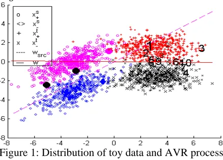
4.1 Toy Data
We generate four bivariate Gaussian distributions as the positive and negative instances of and
[image:3.612.314.533.524.681.2]respectively as illustrated in Figure 1.
Figure 1: Distribution of toy data and AVR process
1
http://people.csail.mit.edu/jrennie/20Newsgroups/.
2
As shown in Figure 1, and randomly sample 1000 instances respectively, then randomly samples 200 instances from . Circle and diamond, big plus and cross, small plus and cross, represent positive and negative instances of
, and respectively.
To this toy data, AVR’s configuration is:
1) , .
2) AVR uses uncertainty sampling to select the least 5 instances which can characterize , to initialize and . In Figure 1, the 5 instances are marked by big filled circles or diamonds, the dash line draws the separating hyperplane 0.
3) Then AVR queries instances as described in Section 3.3, the first 10 queried instances are marked by large numerals, with the first 3 are queried w.r.t. (7). The small numerals mark the first 3 instances which would be queried w.r.t. (6).
4) AVR reweights by (8), where 4. The black filled circles mark the instances whose corresponding c 0. The solid line draws the current hyperplane 0.
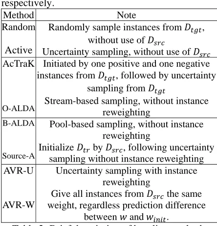
Baseline methods are briefly described in Table 2. Details about AcTraK and ALDA can be found in (Shi et al., 2008) and (Saha et al., 2011) respectively.
Method Note Random
Active
Randomly sample instances from , without use of
Uncertainty sampling, without use of AcTraK
O-ALDA
Initiated by one positive and one negative instances from , followed by uncertainty
sampling from
Stream-based sampling, without instance reweighting
B-ALDA
Source-A
Pool-based sampling, without instance reweighting
Initialize by , following uncertainty sampling without instance reweighting AVR-U
AVR-W
Uncertainty sampling with instance reweighting
Give all instances from the same weight, regardless prediction difference
[image:4.612.312.536.80.188.2]between and .
Table 2: Brief description of baseline methods The first 4 methods referring randomness are run 1000 times to average results as shown in Table 3.
Method Target Domain Labeling Budget
1 2 3 4 5 6 7 8 9 10
Random Active 50.05 49.90 69.35 75.65 79.88 90.41 86.04 95.92 90.26 96.30 93.01 97.23 94.41 97.41 95.30 97.59 96.03 97.64 96.41 97.72 AcTraK O-ALDA 93.15 77 95.23 77 96.10 77.01 96.69 77.07 97.03 77.15 97.30 77.24 97.53 77.33 97.68 77.37 97.78 77.42 97.82 77.48 B-ALDA Source-A AVR-U AVR-W 77 77 80.50 80.50 77 77 95 94 77 77 85 94.50 77 77 96 97 77 77 98.50 98.50 77 77 96 97 77 77 98 98.50 77.50 77.50 98 97.50 77.50 77.50 97 98.50 77.50 77.50 96.50 97
[image:4.612.77.299.426.658.2]AVR 80.50 94 94.50 97 98.50 97 98.50 97.50 98.50 98.50
Table 3: Performance of different methods on toy data, where AcTraK unfairly uses two more labels.
4.2 20 Newsgroups Dataset
20 Newsgroups Dataset is commonly used in machine learning and NLP tasks. It contains about 20000 newsgroup documents which are categorized into 6 top categories and 20 subcategories. We split it into 6 pair of and
, with each pair includes only two top categories documents, such as “comp” and “rec”,
but and are drawn from different
subcategories, e.g. has “comp.graphics” and “comp.graphics”, but has “comp.windows.x” and “sci.autos”. The task is to leverage to distinguish the top categories of documents in . Our settings of 20 Newsgroups Dataset is identical with Dai et al. (2007), details can be found there.
On this dataset, AVR’s configuration is similar with that on toy data, with varies from 500 to 800 on different pairs.
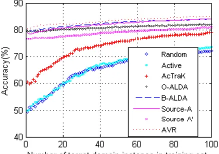
Due to space limit, we only report results on the pair of “comp vs. rec” in Figure 2, with all methods are averaged over 30 runs. The results on other pairs are similar. Since AVR-U and AVR-W are variants of AVR, with similar performance, we only report the results of AVR.
[image:4.612.312.532.532.687.2]4.3 Multi-Domain Sentiment Dataset
The sentiment dataset consists of user reviews about several products (Book, DVD, Electronic, Kitchen) from Amazon.com, the task is to classify a review’s sentiment label as positive or negative. We have 12 pairs with each pair has two products as and respectively. On this dataset, AVR employs VMVPCA (Ji et al., 2011) to project
and , and initializes with
[image:5.612.80.299.339.493.2]1000 instances from w.r.t. (5), while the other configuration is the same as that described in Section 4.1. To be comparable, the baseline methods which leverage are preprocessed by VMVPCA. We also add another baseline method Source-A’ here, which is identical with Source-A, except that it is not projected by VMVPCA. Given space limit, we only report the results on the pair “DVD Kitchen”, with other pairs have similar performance.
Figure 3: AVR does better than previous work on the “DVD Kitchen” dataset for all budget sizes.
4.4 Discussion
From inspection of experimental results, we get the following remarks.
Why to combine active learning and transfer learning?
Active learning such as uncertainty sampling can significantly reduce the labeling cost. But when is far from the optimum, uncertainty sampling may oversample instances near a direction. For example, in Figure 2, Active method is worse than Random method when
50.
could help in learning accurate ,
e.g. in Figure 2, when 200, Source-A method with the help of outperforms Random and Active methods which never use . But inappropriate use of may cause negative transfer, e.g. in Figure 2, when
200, Source-A, ALDA and AcTraK
methods, which overuse , underperform Active method.
Thus, we realize that appropriate combination of transfer learning and active learning could advance and complement each other. Especially when has scarce labels, could help avoid oversample instances near a direction. But with the increase of labels in , should decrease its weight in training to avoid negative transfer.
Does each component of AVR work?
Appropriate Projection of and could mitigate distribution divergence, e.g. in our sentiment classification task, Source-A and AVR which applied VMVPCA significantly and consistently outperforms Source-A’.
Initialize by a small set of critical instances from can significantly reduce training cost without loss of accuracy. E.g. in our experiments, when 1, AVR has better or comparable performance w.r.t. Source-A which initializes by whole . More importantly, AVR trims initial size from 1000 to 5 in toy data, from 4000 to 500 in Newsgroups dataset, and from 2000 to 1000 in Sentiment dataset.
The query strategy of AVR described in Section 3.3 advances traditional active learning, which is supported by the performance of AVR over AVR-U.
Appropriately reweighting instances from and could result in accurate and avoid negative transfer meanwhile. For example, in our experiments, the reweighting strategy of (8) makes AVR outperform all baseline methods, while some of which suffer from negative transfer.
How about AcTraK’s performance?
5 Conclusion and Future Work
Our proposed machine learning framework AVR actively and carefully leverages information of source domain to query the most informative instances in target domain, as well as to train the best possible model of target domain. The four essential components of AVR, which establish its efficacy and help it avoid negative transfer, are validated in experiments.
In the future, we are planning to apply AVR in more tasks with appropriate specification of projection, query and reweighting strategy. Especially for sentiment classification, we will combine prior domain knowledge, such as domain sentiment lexicon, with AVR framework to further reduce labeling cost.
Acknowledgements
This work is supported by the National Fundamental Research Program of China (2010CB327903) and the Doctoral Fund of Ministry of Education of China (20110091110003). We also thank Shujian Huang, Ning Xi, Yinggong Zhao, and anonymous reviewers for their greatly helpful comments.
References
John Biltzer, Ryan Mcdonald, Fernando Pereira. 2006. Domain adaptation with structural correspondence learning. In Proc.EMNLP, pp.120-128.
John Biltzer, Mark Dredze, Fernando Pereira. 2007. Biographies, bollywood, boom-boxes and blenders: domain adaptation for sentiment classification. In
Proc. ACL, pp.432-439.
Rita Chattopadhyay, Jieping Ye, Sethuraman Panchanathan, Wei Fan, Ian Davidson. 2011. Multi-source domain adaptation and its application to early detection of fatigue. In Proc. KDD, pp.717-725.
Wenyuan Dai, Qiang Yang, Gui-Rong Xue, Yong Yu. 2007. Boosting for transfer learning. In Proc. ICML, pp.93-200.
Rong-En Fan, Kai-Wei Chang, Cho-Jui Hsieh, Xiang-Rui Wang, Chih-Jen Lin. 2008. Liblinear: a library for large linear classification. JMLR, 9:1871-1874.
Valerii Vadimovich Fedorov. 1972. Theory of optimal experiments. Academic Press.
David R. Hardoon, Sandor Szedmak, John Shaew-Taylor. 2004. Canonical correlation analysis: An
overview with application to learning methods.
Neural Computation, 16(12): 2639-2664.
Jiayuan Huang, Alexander J. Smola, Arthur Gretton, Karsten M. Borgwardt, Bernhard Scholkpf. 2006. Correcting sample selection bias by unlabeled data. In Proc. NIPS, pp.601-608.
Yangsheng Ji, Jiajun Chen, Gang Niu, Lin Shang, Xinyu Dai. 2011. Transfer learning via multi-view principal component analysis. JCST, 26(1):81-98.
Jing Jiang, ChengXiang Zhai. 2007. Instance weighting for domain adaptation in NLP. In proc. ACL, pp.264-271.
Xuejun Liao, Ya Xue, Lawrence Cain. 2005. Logistic regression with an auxiliary data source. In Proc. ICML, pp.505-512.
Chih-Jen Lin, Ruby C. Weng, S. Sathiya Keerthi. 2008. Trust region newton method for large-scale logistic regression. JMLR, 9:627-650.
David J. C. Mackay. 1992. Information-based objective functions for active data selection. Neural Computation, 5:590-604.
Michael T. Rosenstein, Zvika Marx, Leslie Pack Kaelbling, Thomas G. Dietterich. 2005. To transfer or not to transfer. In Proc. NIPS, December 9-10.
Avishek Saha, Piyush Rai, Hal Daumé III, Suresh Venkatasubramanian, Scott L. DuVall. 2011. Active supervised domain adaptation. In Proc. ECML-PKDD, pp.97-112.
Burr Settles. 2009. Active learning Literature Survey. In
Computer Sciences Technology Report 1648, University of Wisconsin-Madison.
Xiaoxiao Shi, Wei Fan, Jiangtao Ren. 2008. Actively transfer domain knowledge. In Proc. ECML-PKDD
pp.342-357.
Masashi Sugiyama, Shinichi Nakajima, Hisashi Kashima, Paul von B nau, Motoaki Kawanabe. 2008. Direct importance estimation with model selection and its application to covariate shift adaptation.