Munich Personal RePEc Archive
Bounding the productivity default shock
: Evidence from the The European
Sovereign Debt Crisis
Alonso-Ortiz, Jorge and Colla, Esteban and Da-Rocha,
Jose-Maria
1 October 2015
Online at
https://mpra.ub.uni-muenchen.de/67019/
Bounding the productivity default shock : Evidence
from the The European Sovereign Debt Crisis
Jorge Alonso-Ortiz
∗Esteban Colla
†Jos´e-Mar´ıa Da-Rocha
‡June 18, 2014
Abstract
Interest rate spreads on sovereign debt were negatively correlated with the evolution of stock prices during The European Sovereign Debt Crisis. In particular, for a sample of 9 european countries there was a year (between 2009 and 2012) in which the correla-tion between stock prices and spreads was almost -1. We use this fact to estimate the upper bound of productivity default shocks using a continuous time structural model of default. At every instant the government maximizes expected tax revenues, where the only source of uncertainty is TFP, which follows a regime switching brownian motion. By estimating TFP regimes, to match interest rate spreads on sovereign debt and stock prices, we compute the ratio of the productivity if there was a default relative to the no default benchmark. This is a measure on how much productivity could countries loose at default. We found a robust negative relation between the costs of default and the probability of default. That is, financial markets incorporate into prices the risk of default immediately.
Keywords: Default, Sovereign Debt, Financial Markets, Productivity
JEL: E30, E44, G15
∗Instituto Tecnol´ogico Aut´onomo de M´exico (ITAM). Email: jorge.alonso@itam.mx †Universidad Panamericana, M´exico. Email: ecolla@up.edu.mx
1
Introduction
Sovereign defaults are relatively common around the world disrupting the ability of a coun-try to produce value. These episodes may be very costly for the economies that experience them. These costs have been incorporated in the literature as drops in TFP consistent with some key facts, in particular, the fall in GDP that countries experience during a default.1
We can interpret these costs as if they were shocks to productivity originated in a default decision. We will label them as productivity default shocks. After Cole & Kehoe (1996) model of Mexico’s crisis, other papers coincide to set the costs of a default to a fall in TFP of around 5% (Cole & Kehoe, 2000; Da Rocha et al., 2013; Conesa & Kehoe, 2014), but we have little guidance on whether this number is big or not, or by how much could TFP possibly fall in a default episode.
We develop a methodology to estimate the upper bound of productivity default shocks from financial data on stock prices and interest rate spreads. Financial markets are forward looking and reflect new information as it arrives and it is immediately reflected in prices. For example the spot price of an asset reflects the best knowledge about the future prospects of the cash flow that accrue, the interest rate spread reflects the risk of defaulting on debt and so on. Therefore we do not need to observe countries actually defaulting to estimate an upper bound on costs as costs are reflected in stock prices and interest rate spreads. To translate changes in prices into changes in TFP we use the neoclassical growth model, as there is a very simple relation between prices and productivities in the steady state, for standard assumptions on preferences and technology. Changes in prices are changes in TFP augmented by the share of capital and this relationship is invertible, so we can back out information about productivity from stock prices. It is also a model in which most of the default literature is built on.
The European Sovereign Debt Crises brought about a great opportunity to use our method-ology, as some European countries experienced large rises in the risk of default or interest rate spreads on sovereign debt, while their stock prices where falling. We select a sample of European countries from 2009 to 2012, in particular Austria, Belgium, Finland, France, Germany, Ireland, Italy, Netherlands, Portugal and Spain. A key finding in the data is that interest rate spreads on sovereign debt are negatively correlated with the evolution of stock prices. These negative correlations mean that financial markets discount the probability of default on the spot. There is a year for each country in which the correlation between stock prices and spreads is almost -1. We focus in that particular year for each country, interpret-ing the highest negative correlation as a signal sent by financial markets on the likelihood of default. We find large drops in stock prices along spikes in the interest rate spread on sovereign debt. We exploit this information in our estimates.
1
To estimate the upper bound of productivity default shocks we build a continuous time structural model of government default decisions. At every instant the government maxi-mizes expected tax revenues where the only source of uncertainty is TFP, which follows a regime switching brownian motion. Tax revenues are a function of TFP derived through stochastic calculus. We define regime as a drift and standard deviation of the stochastic process, therefore if the government defaults it triggers a change in the mean and variance of the TFP process. A large negative shock to TFP may trigger a permanent change in regime.
The first step of our methodology is estimating the drifts and variances of our TFP pro-cess. We use an algorithm to fit simulated series of stock prices and risk premiums (or interest rate spreads on sovereign debt) from our model to their counterparts found in the data. The second step consists of a Montecarlo exercise to obtain a sample of simulated series for prices with the estimates found in the previous step. We simulate two different series for prices. One for the price of stocks if the country did not default, another for the price of stocks if a country defaulted. Third stage involves transforming our simulated series of prices into simulated series of productivities through the use of the neoclassical growth model in the steady state. Once we have these simulated series of productivities we compute the ratio of the productivity if there was a default to the productivity if there was not a default. This gives us a measure of how much productivity countries loose if they default. As we drew many observations in our Montecarlo stage we average our series and compute standard deviations. The mean of this ratio over our period of estimation is a measure of how much would TFP fall if a country defaulted. The standard deviations will be essential to our notion of upper bound.
Finally we regress the probability of default over our measure of productivity default shocks for each country in the period of time we selected. We need this final step because none of the countries in our sample defaulted but it was likely that some did. Our regression spells out what the average costs of productivity default shocks would be. Therefore we are estimating a rule rather, or a prediction function, than a number. A key feature to find our rule is the robust negative correlation between the costs of default and the probability of default that we find in the data and in the model. To construct the upper bound on the productivity default shocks we subtract the standard deviations, found in step 3, times 1.96 to our rule. This will be our upper bound.
Our main motivation, and our contribution as well, is providing alternative estimates on how much a country can potentially loose, in terms of productivity, if it chooses to default. Many papers that find moderate cost of default are based upon real default episodes in emerging economies. Therefore it is not clear if a permanent fall in TFP of 5% is the cost that countries actually take into account when they evaluate a default decision, which are made under uncertainty. Therefore countries take into account what these costs could be before a default decision is made. Our findings point to large potential permanent drops in productivity in case of a default. However moderate drops in productivity, as those found in the macro literature, are perfectly consistent with our results.
As far as we know the only paper related to ours is Glober (2013) that deals with a similar problem but for US business debt. In his paper he estimates what the expected cost of de-fault is for US businesses. Using a continuous time model of firms dede-fault decisions, subject to a regime switching firm productivity process, he finds that the average costs of default is 45% in terms of the value of firms, whereas previous estimates in that literature place the average costs at 25%; almost half. The probability of default on private debt is generally higher than on sovereign debt. If the weight of capital in GDP is a third, 45% change in the value of a firm is equivalent to a 28% change in TFP. Previous literature were finding a TFP equivalent number of 19% according to the neoclassical growth model. Therefore our results on cross country productivity costs of default are consistent with the findings in the default on private debt literature.
In section 2 we present the model that we use to estimate regime switching parameters of the underlying TFP process. In section 3 we present the data that is needed to estimate TFP parameters and feed the model. Section 4 present main results and Section 5 concludes.
2
Model
We build a model of government default decisions to estimate what are the regime switching parameters that characterize TFP. In our model government’s default decisions affect the productivity of the economy through a change in the drift and variance parameters of the productivity process. Our model is written in continuos time as we will use daily data for our estimation and because it will let us write down parts of the model in close form.
2.1
Firms and Productivity
We assume a representative firm which is, in fact, a productivity process. This process is written down as a geometric Brownian motion.
dA=µsAdt+σsAdzt
government’s dichotomous default decisions s ∈ {d, nd}, where s =nd stands for the state of the economy with no default and vice-versa. In case of a default productivity drift and variance switch to a different regime and stays there forever.2
2.2
Government Problem
The government is the only decision maker in our model. At every time, government faces the following cash-flow equation
θA−g+ [q(A)−1]b.
that depends on a tax rateθ over the value of the firm, government expenditureg and debt
b, where q(A) is the state dependent price of bonds. Taxes are usually levied over income or consumption but we will choose the tax rate so it is consistent with fiscal data for our period of estimation.
Taking cash flow as given the government faces an optimal stopping problem. It may choose to role over its debt over the period or it may choose to default. The value of defaultWd(A)
is the present value of the primary deficit, therefore bond markets are closed forever, which could be interpreted as a capital flight to a safe asset (i.e. the german bond) that we are not explicitly modeling. The value of default can be written in closed form as an integral of a stochastic process:
Wd(A) =
Z ∞
d
(θA−g)e−(r−µd+σ
2
d/2)tdt= θA
r−µd+σ2d/2
− g
r
Formally, the optimal stationary stopping problem can be written down as:
W(A) = max
d∈{0,1}
θA−g+ (q(A)−1)b+ (1 +rdt)−1EW(A+dA), Wd(A)
s.t. dA
A =µnddt+σnddz
where the instantaneous cash flow plus its continuation value is compared to the value of defaulting.
As a result we will obtain a stationary stopping rule that is a threshold value ˆAd for
produc-tivity. If A falls below this threshold, the government will choose to default and stay in the default region forever.
We can write down the government’s value of repaying W(A) as an ordinary second or-der stochastic differential equation
2
rW(A) =θA−g+ [q(A)−1]b+µndAW′(A) +
σ2
nd
2 A
2W′′(A)
with a boundary and smooth pasting conditions
W(Ad) =
θAd
r−µd+σd2/2
− g
r
W′(Ad) =
θ r−µd+σd2/2
which means that the value function of no defaulting, evaluated at the default threshold, and the value of defaulting are equal. We also impose a smooth pasting condition which is needed to solve this kind of problems (Dixit & Pindyck (1993))
2.3
Risk Premium
Risk premium is equal to the difference in returns between the bond and a risk free asset
1
q(A)−(1 +r)
whereris the risk-free rate of return andq(A) the price of the issued bonds, which is related to the government decision through the productivity process. Using Ito’s lemma we can write down q(A) as a solution to a partial differential equation:
rq(A) = µndAq′(A) +
σ2
nd
2 A
2q′′(A)
subject to the following boundary conditions
q(Ad) = 0
lim
A→A∗q(A) =
1 1 +r
Note that the first boundary condition follows from the assumption that after a default, bond holders are not repaid, therefore the price of bonds is zero. The second boundary con-dition states that the price of a risk-less bond is (1 +r)−1 whereA∗ is the safety productivity
level3. After solving this equation, we can substitute q(A) in the government’s problem and
obtain the productivity threshold Ad.
3
2.4
Firm’s Value
As in a standard asset pricing model in continuous time the value of the representative firm is related with the evolution of its fundamental. In this particular case the firm’s value is a regime switching stochastic process. In case of no default the value of a firm is made up of the instantaneous return plus the expected change in the value of the firm. The expected change depends on the probability of default p(A)
rVnd(A) =µndAVnd′ (A) +
σ2
nd
2 A
2V′′
nd(A) +p(A) [Vd(A)−Vnd(A)]
with boundary and smooth pasting conditions
Vnd(Ad) = Vd(Ad)
Vnd′ (Ad) = Vd′(Ad)
In case of default, the value of the representative firm can be written down as
rVd(A) =µdAVd′(A) +
σ2
d
2 A
2V′′
d(A)
with boundary conditions
Vd(0) = 0
Vd′(0) = 0
Note that in case of default there is no further changes in regime.
To be able to compute the value of the firm in case of no default we need to solve for the value of the firm in case of default and the probability of default. If the government had defaulted, the value of a firm can be solved in closed form as Vd(A) =Aβd, where βd is the
positive root of σ
2
d
2 β2+ (µd−
σ2
d
2 )β−r = 0.
The probability of default can be obtained through solving the following partial differential equation
0 =−µndAp′(A) +
σ2
nd
2 A
2p′′(A)
with boundary conditions
p(Ad) = 1
lim
A→∞p(A) = 0
The first boundary condition tells us that if A≤ Ad then the probability of default is zero,
similarly if A → ∞ the probability of default is zero. We can solve this equation in closed
form as p(A) =AA
d
−
1−2µnd σ2
nd
To solve for Vnd(A), we rewrite the switching problem through the following change of
variable x= log (A/Ad)
"
r−e−
1−2µnd σ2
nd
x
#
Vnd(xt) = ˆα1Vnd′ (xt) +
σ2
nd
2 V
′′
nd(xt) +e−(1−
2µnd
σ2 )xAβ0
d eβ
0x
where boundary conditions are given by
V1(0) = Adeβ0
V1′(0) = β0Adeβ0.
and the probability of defaulting is equal toe−(1−
2µnd
σ2 )x. As a result of this solution process
we have endogenous process for productivity, the value of the firm, the risk premium and the probability of default. We will use these simulated series to match their corresponding series in the data.
3
Data and Calibration
3.1
Data
We collect data for 9 European countries: Austria, Belgium, Finland, France, Germany4,
Ireland, Italy, Netherlands, Portugal and Spain. These countries fared relatively well and homogeneously before the 2007’s great recession but they had quite heterogeneous perfor-mances during and in the down of this recession. Therefore this is a great opportunity to exploit this heterogeneity to learn what would the costs of default be.
We focus on financial data, in particular, series of stock price indices and 10-Y Bond in-terests rates, as they reflect the probability of default on sovereign debt. We also compute series of the probability of default for each country,Pj using Germany as the risk free option
Pj = 1−
Rj
Rger
where R stands for the interest rate of 10-Y Bond in each country, therefore Germany is considered to have a zero probability of default.
We will also need data on the value of debt and tax rates for each country to feed our model. Figure 1 shows two countries, Austria in 2009 and Spain in 2012 as an example, but a similar pattern can be found for every country in our sample during 2009-1012. Austria is representative of the group of countries that performed better in the recession (Finland, France, Germany), whereas Spain is a example of the countries that performed worse (Por-tugal, Italy, Ireland). It is worth noting that there is a large negative correlation between
4
Figure 1: Stock Prices and Risk Premium
(a) Austria 2009 (b) Spain 2012
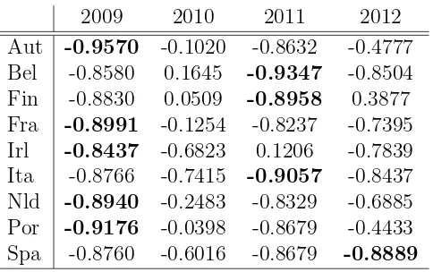
stock prices and the 10-Y Bond interest rate, meaning that when markets discount a larger probability of default the price of stocks fall in a larger amount. This may be a hint that financial markets believe the country is going to default. To exploit this source of identifica-tion we select a year, for each country, when the correlaidentifica-tion of the stock prices and interest rate is larger in absolute value. Table 1 shows the correlation for each year and each country.
Therefore we select Austria in 2009, Belgium in 2011, France in 2009, Ireland in 2009,
Table 1: Correlation Stock Prices vs. Risk Premium
2009 2010 2011 2012 Aut -0.9570 -0.1020 -0.8632 -0.4777 Bel -0.8580 0.1645 -0.9347 -0.8504 Fin -0.8830 0.0509 -0.8958 0.3877 Fra -0.8991 -0.1254 -0.8237 -0.7395 Irl -0.8437 -0.6823 0.1206 -0.7839 Ita -0.8766 -0.7415 -0.9057 -0.8437 Nld -0.8940 -0.2483 -0.8329 -0.6885 Por -0.9176 -0.0398 -0.8679 -0.4433 Spa -0.8760 -0.6016 -0.8679 -0.8889
Italy in 2009, Netherlands in 2009, Portugal in 2009 and Spain in 2012, as we highlight in boldface in Table 1; for most countries, it is above .90. These are the years that we will use for the estimation of TFP processes in each country.
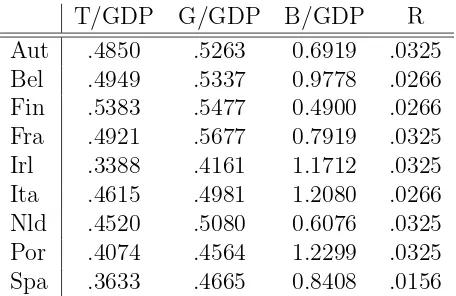
[image:10.612.187.429.444.596.2]ratio. We use IMF’s World Economic Outlook Database to collect data on tax revenues, government expenditure and debt-GDP ratio. Table 2 shows these data for the period that we selected for each country. We need data on taxes and government expenditure to construct
Table 2: Fiscal Policy Parameters and Risk Free Rate
T/GDP G/GDP B/GDP R Aut .4850 .5263 0.6919 .0325 Bel .4949 .5337 0.9778 .0266 Fin .5383 .5477 0.4900 .0266 Fra .4921 .5677 0.7919 .0325 Irl .3388 .4161 1.1712 .0325 Ita .4615 .4981 1.2080 .0266 Nld .4520 .5080 0.6076 .0325 Por .4074 .4564 1.2299 .0325 Spa .3633 .4665 0.8408 .0156
a measure of deficits. We need data on risk free interest rate (Germany) and government debt to obtain the service of debt. With deficits and the service of debt we construct a measure of government cash flows, which is the objective function that each government tries to maximize in our model written down in Section 2.
3.2
Calibration
We need to calibrate eight parameters that we divide in two groups. The first group are pa-rameters that are directly taken from data, as the debt-GDP ratiob, government expenditure-GDP ratio g, government revenue-GDP ratiotand risk free interest rate r, which are shown in Table 2. The other group of parameters, θ, µi and σi, for i ∈ {d, nd} is chosen to match
several statistics in the data. We choseθ, which is the tax rate in our model, to satisfy that marginal government revenues
W′(A) = θ
r−µd+σd2/2
=t
match the government revenue-GDP ratio. Of course we are assuming in this case that average taxes equal marginal taxes. Our results do not rely on this assumption at all, better estimates of marginal tax rates (as in McDaniel (2013)) are not so far-off from average taxes to matter in the period of time we are considering.
The parameters of the productivity stochastic process: µnd, σnd, µd, σd are chosen to
mini-mize the square deviation of normalized5 stock prices and risk premium series, the variance
5
of stock prices variance of stock prices and the variance of risk premiums. We solve this problem numerically using through the following algorithm.
Calibration Algorithm: Given some initial guess on the vector {µ0
nd, σ0nd, µ0d, σd0}:
(i) We compute the default threshold ˆA0
d
(ii) We simulate series for A0
nd, A0d and p( ˆAnd0 ). If at some point A0nd ≤ Aˆ0d a country
enters in default, jumping from A0
nd to A0d (iii) Given (ii) we compute series of the value of
firms V(A0
i) where ican be default or no-default
(iv) Given (iii) we compute the mean quadratic deviation of the simulated series V(A0
i)
and p( ˆA0
nd) to their data counterpart
(v) Given (iv) we use a minimization routine to update parameters to {µ1
nd, σnd1 , µ1d, σ1d}
Our algorithm involves the solution of a system of stochastic differential equations which in general could admit more than one solution. Furthermore, we are embedding this prob-lem into an objective function that could potentially have many local minima. To best circumvent these problems, we use a minimization procedure based on a genetic global search algorithm. These algorithms require to bound the parameter space to narrow a time consuming search. Our criteria to bound the parameter space are common sense and the evo-lution of TFP resulting from a development accounting exercise to back our common sense. For example, we set bounds on drifts and standard deviations of the TFP process so that they are not much larger to the TFP falls in the accounting exercise. The bounds that we set did not bind in any of our trials, so bounding the parameter space do not affect our results.
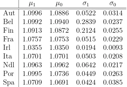
[image:12.612.202.412.524.669.2]Calibration Results: Table 3 shows our calibrated drifts in annual terms and standard deviations. We annualize drifts so they are easier to understand For mostly every country
Table 3: Annualized Calibrated Parameters
µ1 µ0 σ1 σ0
drifts fall, in case of a default, but most of the action comes from changes in the standard deviation of the stochastic process. It looks like for many countries the standard deviation falls substantially in case of a default. Therefore most of the action comes from changes in the variance of the stochastic process. We illustrate the fit of our model to the evolution of stock prices in Figure 2, following our example of Austria and Spain. These two countries
Figure 2: Stock Prices and Risk Premium
(a) Austria 2009 (b) Spain 2012
are particularly interesting because the fit for Spain is fairly good, whereas the fit for Austria is worse. Note that our objective is not to fit stock prices, but a nice feature of our model is that it fits data relatively well, given its simplicity. Even though there is not equivalent notion of r-square we can compute the ratio of the volatility of simulated series relative to the volatility of data. We find that volatility in data relative to simulations is close to 1. Sometimes our simulations over-predict volatility, as in Austria and Spain, with ratios of 1.16 and 1.19, sometimes we under-predict as in Finland, with a ratio of .84.
4
Bound on the Productivity Default Shocks
To bound the productivity default shocks we developed a methodology to extract informa-tion from stock prices and risk premiums. We will divide our methodology in steps to ease understanding. First we use our model to estimate what are the parameters that charac-terize the TFP stochastic process in our model. Second, we run a Montecarlo experiment to obtain a sample of simulated series for stock prices. We simulate two different series of prices. One for the stocks prices if the country did not defaulted and another for stock prices if a country defaulted. The third stage involves transforming our simulated series of prices into simulated series of productivities through the use of the neoclassical growth model in a steady state equilibrium.
as
yit=Aitkitα
where α is the capital share and i stands for whether a country is in default or not. We assume that labor supply is inelastic and equal across countries. This assumption is not important as we care about the ratio of the value of firms in case of default and no default in each country, so the labor input cancels out. We will use the definition of the price of a firm in the steady state to back out productivity numbers.
The standard solution that we give to our students in intermediate to advanced courses in macroeconomics is that the price of a firm in a steady state equilibrium is the value of its capital stock in the steady state. This capital stock can be written as
vit∗ =
αAit
ρ+δ
1−1α
whereρ is the discount rate andδ is the depreciation rate of the capital stock. Therefore we can write the ratio of the price of a firm in default relative to its price in no-default as
v∗ dt v∗ ndt = Adt Andt
1−1α
which allow us to measure changes in productivity inverting the previous expression
Adt Andt = v∗ dt v∗ ndt
1−α
where we will assume that α = .4 which is relatively standard in the literature. Once we have the ratio of productivities in default relative to no-default, we average them out and compute their standard deviations. Standard deviations are particularly important because they will give us a statistical notion on what is the highest bound to productivity default shocks.
This is not enough to compute productivity default shocks because none of the countries in our sample have defaulted, but financial markets thought it was very likely. This leads to our final step. We use this insight to compute a measure of the magnitude of productivity de-fault shocks. We regress our measure of changes in TFP on the probability of dede-fault across countries Pj defined in previous section, where j stands for each country in our sample, as
Ad
And
j
=a0+a1∗Pj +ǫj
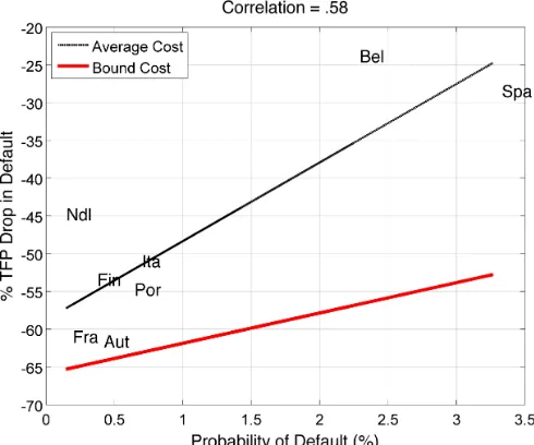
Figure 3: Probability and Costs of Default
out productivity default shocks, given probabilities of default. A key insight of our paper is that we can not estimate the costs of default as numbers because they are not independent of how likely it is that a country defaults. This is due to the forward looking nature of financial markets. Take the same two countries that we have been using as examples: Austria in 2009 and Spain in 2012. Austria had a probability of default below .5% as markets did not consider likely that it defaulted. Regardless of how unlikely this event was, if it happened, it would have costed Austria 55% of its productivity relative to no-default. On the other hand Spain had a probability of default above 3.5% and its productivity would have fallen by 22% at default. As the probability of default was high(er) for the spanish economy, markets had already discounted it, imposing costs to the economy in terms of productivity before a default that never happened.
These costs are clearly not the highest that a country should reasonably expect, which is what we are after. To compute by how much could TFP fall in case of default we con-struct confidence intervals over the average productivity default shocks. There is no known distribution for the ratio of productivities but we use the standard deviations of this ratio, computed through Montecarlo simulations and choose the cut off value of a normal distri-bution for a 95% level of confidence (1.96). The upper bound is of no interest to us but the lower bound is represented as a bold red line in Figure 3.
would have fallen by no more than 50% (twice the average cost).
[image:16.612.197.414.196.285.2]Our results depend on the assumed value forαbut Table 4 shows bounds on the productivity default shock for different values ofα. If is well know (Gollin (2004)) that labor shares do not differ that much across countries, once we have into account proprietors income. However, we show that results are sensitive to the capital share that we assume. As capital rises,
Table 4: Bound on Productivity Default Shocks Capital Share
P (%) 0.4 0.5 0.6 0.7
2 -56.39 -50.16 -39.77 -34.47 3 -46.34 -40.58 -31.39 -26.65 6 -36.30 -31.01 -23.01 -18.83 9 -21.24 -16.64 -10.44 -7.10
productivity matters less to determine the value of a firm and changes in the price of firms (or the value of the stock of capital) do not generate such big costs in terms of productivity. For example in a country with a capital share of .4, if the probability of default were 2% the maximum productivity default shock would be 56%, whereas if the probability of default were 9% the maximum productivity default shock would be of 21%. However if capital share were .7, costs of default shocks would be much smaller. For the same probabilities of default of 2 and 9% the costs of default are much smaller would be 35% versus 7% respectively.
One of the first papers to compute a default productivity shock for a given probability was Cole & Kehoe (2000). In their paper they find that for a 2% probability of default and a capital share of .4, the magnitude of default shocks in terms of productivity is 5%. Most of the papers from there on have found that 5% seems to be a reasonable number, when studying default episodes in emerging economies. Take for example Argentina. Da-Rocha et. al (2013) write down a model of self-fulfilling crises with default and devaluation. In their calibration they find costs in terms of productivity of 5% with a probability of default of 4.7%, using a capital share of .3. Clearly this is below the maximum costs that could have been of 40%. Yue (2010) finds that the costs of default are 7% for a probability of default of 2.7%. Similarly, Arellano (2008) find a deviation from trend of 9% from GDP with a probability of default of 3%.6 It is worth noting that if we take these three papers’
numbers we can see a negative correlation between the calibrated costs of default and their probabilities, consistent with our findings in this paper.
There are many factors, not captured by our model, which may impact the relation be-tween productivity default shocks and the probability of default. Countries are not excluded forever from financial markets. Eventually their reputation improves and the rest of the
6
world start lending that country again. Countries that are going to default are also subject to many policy interventions from their national government, their central bank and interna-tional organizations, such as the IMF. In Europe the ECB and the EU (specially Germany) intervened in greek and spanish debt markets to reduce the risk of default. These type of interventions may affect the cost of default when it happens but they are not the focus of this paper.
5
Conclusions
In this paper we developed a methodology to extract, from financial data (stock prices and risk premiums), information about how big the productivity costs of a default shock may be. We use a sample of european countries involved in the region sovereign debt crises. In particular, we focus on the period from 2009 to 2012, which is a time span when correlations between risk premiums and stock prices were highest.
Our methodology consists of estimating regime switching productivity parameters, drifts and variances, using a continuos time model of government default decisions under uncer-tainty. With the estimated parameters we turn into simulating series of stock prices in case of default and no-default. We define a measure for costs of default shocks interpreting our data through the lenses of the neoclassical growth model.
We find a rule that spells out certain productivity default shock for a given probability of default. Countries in which the probability of default is small find that default productiv-ity shocks will be large, as markets were not expecting default from such country. However, if the probability of default for a country is high default productivity shocks will be smaller, as financial markets discounted such an event from the price of stocks.
6
References
1. Arellano, C. (2008) “Default Risk and Income Fluctuations in Emerging Economies.” American Economic Review, 98:2, 690-712
2. Bai, Y. & Zhang, J. (2012) “Duration of sovereign debt renegotiation.” Journal of International Economics, 86: 252-258.
3. Cole H.L. & Kehoe, T.J. (1996) “‘A Self-Fullfilling Model of Mexico’s 1994-95 Debt Crisis,” Journal of International Economics,41, 309-30
4. Cole H.L. & Kehoe, T.J. (2000) “Self-Fulfilling Debt Crises.” The Review of Economic Studies, 67, 91-116
6. Da-Rocha, J.M., Gimenez, E.L. & Lores, F.J. (2013) “Self-fulfilling crises with default and devaluation.” Economic Theory. Vol. 53, 3: 499-535
7. Dixit, A.K. & Pindyck, R.S. (1994) “Investment Under Uncertainty.” Princeton Uni-versity Press
8. Glover, B. (2013) “The Expected Cost of Default.” Mimeo
9. Gollin, D. (2002) “Getting Income Shares Right.” Journal of Political Economy. Vol. 110. No. 2, pp. 458-474 Kehoe T. J. and Ruhl K. J. (2009) “Sudden Stops, Sectoral Reallocations, and the Real Exchange Rate,,” Journal of Development Economics, 89, 235-249.
10. McDaniel, C. (2011) “Forces Shaping Hours in the OECD.” American Economic Jour-nal: Macroeconomics. Vol. 3 (4)
11. Mendoza, E.G. & Yue, V.Z. (2012) “A General Equilibrium Model of Sovereign Default and Business Cycles.” The Quarterly Journal of Economics, 127, 889-946