On the Samuelson Etula Master Function and Marginal Productivity: some old and new critical remarks

On the Samuelson-Etula Master Function

and Marginal Productivity: some old and

new critical remarks

Dvoskin, Ariel and Fratini, Saverio M.

University of Buenos Aires-CONICET, Roma Tre University

April 2015

Online at

https://mpra.ub.uni-muenchen.de/63415/

‘the danger lies in this, that when we have succeeded in thoroughly

mastering a technique, we are very liable to be mastered byher.’

Piero Sraffa (D3/12/4:15)

On the Samuelson-Etula Master Function and Marginal

Productivity: some old and new critical remarks

Ariel Dvoskin* & Saverio M. Fratini**

(*University of Buenos Aires-CONICET; **Roma Tre University)

ABSTRACT

The paper addresses the ambiguity that surrounds the conception of capital and its role in neoclassical price-and-distribution theory. The difficulties encountered in the various attempts to define the marginal product either of capital or of a capital good are recalled and the conclusion is drawn that neither concept appears theoretically sound. This is combined with critical discussion of the recent attempt by Samuelson

and Etula to determine income distribution by means of their ‘Master

Function’ and its ‘non-neoclassical’ marginal products. Rather than the existence of a continuum of alternative technical possibilities, Samuelson and Etula assume the simultaneous coexistence of a discrete number of methods of production for the same commodity. Even though each technique employs the inputs in fixed proportions, the coexistence of various techniques permits the full employment of an arbitrarily given vector of input endowments. As is shown here, however, the coexistence of methods required for the differentiability of the Samuelson-Etula Master Function can take place, if capital goods are used in production, neither in the case with stationary relative prices nor in the non-stationary Arrow-Debreu framework.

JEL Codes: B21 – C61 - D24 - D46 – D51

Keywords: capital – capital goods – marginal product of capital – Master Function -

Introduction

Capital is unquestionably among the principal sources of controversy in economic theory and the long list of authoritative economists involved includes scholars like Böhm-Bawerk, J.B. Clark, Hayek, Knight, Hicks, Samuelson, Solow, Pasinetti and Garegnani in different periods.

While the specific issues differ in the course of the various disputes, their common root can be found in the ambiguity that surrounds the conception of capital and its role in the neoclassical-marginalist theory of value and distribution. As this ambiguity still remains unresolved, new disputes periodically arise when attempts are made to define a ‘new’ concept of marginal product of capital and prove its equality, in equilibrium, with the rate of interest. Such attempts include the Samuelson-Etula Master Function and its partial derivatives, which are discussed here.

The analysis begins in section 2 with a discussion of the ambiguity in question. It is argued that a major source of misunderstanding and confusion is the fact that capital, which actually means the amount of purchasing power making it possible to finance the costs of production, has often been understood as a synthesis of the capital goods employed as

inputs in the production process. This gives rise to the false impression – and hope – that these goods can be aggregated into a single input called ‘capital’.

In a nutshell, the ambiguity over two different objects, namely capital and capital goods, has given rise to a purely ideal conception, a sort of Holy Grail of economic theory, which can be called ‘aggregate capital’, a factor of production to be employed together with and with the same role as labour and land. If such an aggregate capital existed, then its marginal product, in equilibrium, would be equal to the rate of interest, just as the marginal products of labour and land would be respectively equal to the rates of wage and rent.

In actual fact, however, unlike labour and land, capital is not an input but simply an amount of value that allows firms to finance their costs of production. While capital goods

are instead inputs, their employment cannot be aggregated into a homogenous mass without illegitimate ‘hyper-simplification’.

argued in section 3, however, the fact that capital goods are both complementary to other inputs and highly specialized poses serious obstacles to the construction of a production function that has capital goods as independent variables and whose partial derivatives could be used to determine income distribution.

Sections 4 and 5 examine a recent series of articles by Samuelson and Etula (Samuelson, 2007; Etula, 2006; Samuelson and Etula, 2006) in which, despite these difficulties, an attempt is made to use their ‘Master Function’ – a production function that includes the vector of capital goods among its arguments – to determine income distribution by means of what the authors call the function’s ‘non-neoclassical’ marginal products. The conclusion drawn here is that the attempt is unsuccessful, at least in the general case in which capital goods are taken into consideration. As a result, contrary to the authors’ claims, the explanation of income distribution by means of the Master Function’s partial derivatives cannot be generally accepted.

The demonstration of this begins by considering the stationary framework in which Samuelson and Etula embed their analysis and showing that a problem of consistency emerges in that context between the stationary hypothesis and the non-uniformity of the rates of return of capital goods, which is generally implied by the need for the coexistence of a sufficient number of methods to allow full employment of the arbitrarily given endowment of inputs. A non-stationary Arrow-Debreu framework is then examined and it is shown that in this case, full employment of the initial endowments does not imply utilisation of the sufficient number of methods to obtain a differentiable Master Function.

2. On the notion of capital once again

The primary aim of this section is to disprove this view by showing that value capital on the one hand and capital goods on the other are not in general two sides of the same coin but two different things. As we shall see, the distinction between value capital and capital goods is not merely a matter of the way in which the theorist chooses to represent capital but rather reflects a difference in nature and role.

Let us start from the beginning. Production takes time. Inputs are employed before outputs are obtained, as cause must precede effect. In accordance with a standard representation of production, the case can therefore be imagined in which a series of inputs – i.e. various commodities (capital goods), different kinds of labour services and the use of different sorts of natural resources – are employed in a certain process in period t and a series of outputs – commodities – are obtained as a result in period t+1.

It can be stated in terms of a standard notation1 that a vector of quantities of inputs at is employed in t and a vector of quantities of outputs bt+1 is obtained in t+1. If pa is the (row) price vector of inputs, then pa ∙ at represents total production cost. Similarly, if pb is the (row) price vector of outputs, then pb∙ bt+1 is the amount of revenue (and the difference

 = pb∙ bt+1pa∙ at stands for profit).

If it is assumed that inputs are bought onto the market in the period in which they are employed and that outputs are sold in the period in which they are obtained, the costs and revenues of the same process do not manifest themselves simultaneously. Entrepreneurs therefore cannot use revenues to finance costs because costs and revenues are related to different market days. Capital is what allows entrepreneurs to buy inputs on the market in period t and it is therefore an amount of purchasing power. Subsequently, in period t+1, when the outputs are sold, revenues reimburse the capital with a profit.2

If the costs can instead be paid – totally or partially – on the same market day as the outputs are sold, then no capital is needed in that payment. This is what happens, for example, if it is assumed that wages are paid post factum, i.e. in the moment in which the

1

In particular, we refer to the notation introduced by Malinvaud (1953). 2

As the reader will have noticed, this is the notion of capital found, among others, in Marx with the money-commodities-money triad. A sum of money M, i.e. purchasing power, is initially turned into an amount (or vector) of commodities, C. This is done directly, in the case of merchants’ capital, or indirectly, by buying the inputs that produce the commodities, in the case of industrial capital. The commodities are then turned back into a sum of money M’. This is because capital ‘is not spent, is

merely advanced’ (Marx 1909, vol. I, p. 166) and therefore returns to the capitalist augmented by

outputs are obtained and sold. Another example is provided by the models in which all markets, for both current and future delivery, are assumed to open for a single instant, as in the Arrow-Debreu model, so that the inputs and outputs of the same process are traded simultaneously. In this case too, costs can be met directly out of revenues and no advance financing by capital is needed.

Two observations follow from the above. First, capital is an object of the same kind as costs and revenues. Capital is an amount of purchasing power, i.e. an amount of value, and as such it is not an input. Unlike labour and land, it is not in a technical relationship with outputs, as clearly shown by the fact that while it is always possible to express the employment of labour and land in ‘technical units’ – i.e. in such a way as to have a non-ambiguous relationship between each of them and the amount of output3 – this possibility does not exist for the employment of capital. The problem is not simply that value is not a technical unit of measure but rather that capital is not an input. The lack of a technical unit of measure for it is simply a consequence of this fact.4

Second, capital goods, which are better referred to as means of production in order to avoid any ambiguity, are inputs. In the absence of specific assumptions, however, they cannot be regarded as the physical counterpart of capital or as what capital is spent on or invested in. Capital is spent to purchase all the inputs in vector at, which includes means of production but also the production services of various sorts of labour and natural resources. Capital is invested in financing the costs of production of certain outputs, totally or partially.

Means of production can be regarded as the real assets into which capital is converted5 only on some ad hoc assumptions. In particular, it can be assumed that a) wages and rents are paid at the end of the production process or that b) wages are regarded in physical terms ‘as the fuel for the engines or the feed for the cattle’ (Sraffa 1960, p. 9) and

3

To give just one example, if the employment of labour is expressed – as it should be – in terms of labour hours, then an increase in the employment of labour brings about an increase in the amount of output, ceteris paribus,. If it is instead expressed as the sum of the heights of all workers, then the relationship between labour employment and output is ambiguous, as no general conclusion can

be drawn about the effect of an increase in workers’ total height on output.

4

It is clear that if capital were an input, its technical unit of measure could be deduced directly from the observation of reality, as is the case for all true inputs.

5

rents do not enter into the costs of production. Assumption (a) is typically neoclassical6 while assumption (b) has a classical flavour, but in both cases capital is used to buy a set of commodities.7

These assumptions have certainly helped to generate the ambiguity mentioned at the beginning of this section and in particular to spread the erroneous idea that capital is an input and can be conceived in both ‘aggregate’ and ‘disaggregate’ terms. It should now be clear, however, that capital is the amount of purchasing power that makes it possible to finance production costs (totally or partially) and must not be confused with the means of production or capital goods, which play a different role. This distinction should be preserved even – or especially – when the value of the means of production is the only part of the costs financed by capital.

There is no shortage of claims in the 20th-century literature on capital theory that the problem is one of expressing capital as a single magnitude. On the one hand, this is somewhat surprising because capital is a single magnitude, namely an amount of purchasing power. On the other, if the real problem is – as the present authors believe – one of expressing a vector of capital goods as an amount of ‘aggregate capital’ in order to regard it as an input on the same footing as labour and land, then it is not simply a ‘problem’ but an impossible task, as a vector cannot be expressed by a scalar. Various attempts in this direction can be mentioned, from the average period of production of Jevons and Böhm-Bawerk to the ‘Meccano sets’ of Swan (1956) and the ‘jelly’ of Samuelson (1962), as discussed in the next section. As is known, none of these attempts has worked. The possibility of ‘synthesising’ or ‘aggregating’ capital goods in general into a single factor of production is nothing more than an illusion.8

6

The neoclassical theory of distribution tends – at least in its initial formulations – to see wages and rents in the same terms as profits (interests). As a result, since profits appear in the same moment as outputs are sold, it is also are assumed that wages and rents are paid in that moment.

7

It is worth noting that in these two cases, the transformation of capital into commodities does not have the same meaning as the Marxian M-C-M’. The Cin Marx’s expression is not in fact a vector of inputs but rather a vector of outputs that is sold for the amount of money M’. The Marxian transformation of M into C– and then of C into M’– therefore requires no ad hoc assumptions and is decidedly general. On the contrary, the conversion of capital into a vector of means of production necessitates either assumption (a) or assumption (b).

8

3. Marginal equalities and capital goods

There is no need here to enter into an analysis of the meaning and role in neoclassical theory of marginal productivity and its equality with the price of inputs. Those interested are referred to the extensive literature already existing on these matters. For our present purposes, it will suffice to recall very briefly just a few points.

If, given the technical conditions of production, the quantity of a certain output can be expressed as a differentiable function of the quantities of inputs employed in its production, then the equalities between the marginal products of the latter and their relative prices in terms of output (marginal equalities) are the first-order conditions of a standard profit-maximisation problem. Marginal equalities have thus been used by neoclassical theory as a possible basis for the claim that the demand for inputs depends on their relative prices and a supply-and-demand equilibrium can therefore be attained through their adjustment. This is indeed the way in which distributive variables – interpreted as factor prices – are determined according the neoclassical-marginalist theory.9

 = , , , …, each producing the same final output (consumption good) and denote as y and k +n respectively the net product and the vector of capital goods, both understood per unit of labour. The aggregation of capital goods consists in turning the vector k_ into a scalar s_. In other words, it

consists in finding a vector vn such that vk = s. This aggregation is, however, problematic in many respects.

First of all, it may happen that i) s = s but y≠ y, ii) s≠ s, but y = y or iii) s > s, but y

< y. It is clear in these cases that aggregation brings about a loss of relevant information about the relationship between inputs and output: s_ does not provide enough information to explain y. Second, if the price vector is used as vector v so that s_ = pk_, new problems arise. With r as the rate of interest, it is possible to have iv) ds / dr > 0 and v) s > s if r = r’ and s < s, if r = r”,

with r’ ≠ r”. (It should be noted that (iv) is called ‘reverse capital deepening’, while (v) has no

name.) In conclusion, there is thus impossible in general to say that one technique is more capital-intensive than another in anything other than tautological terms.

9

As has been known since the publication of Wicksell’s Lectures ([1901] 1934), capital is not an input and therefore cannot appear among the independent variables of a production function, or at least not if this function is viewed exclusively as the expression of the technical conditions of production. Various attempts have been made, however, to obtain an indirect or ‘surrogate’ marginal product of capital. In these cases, a variation in the rate of interest is usually assumed with changes in the methods of production in use and in the price system arising as a result. There are thus variations both in the quantity of output and in the investment of capital – with a given employment of labour – and the ratio between them has been interpreted as a ‘marginal product of capital’. Moreover, if an equilibrium position is taken as the starting point and changes in the price system due to the variation of distribution are overlooked, this particular marginal product of capital proves to be equal to the rate of interest, thus giving the false impression of a marginal equality (see for example Malinvaud, 1953, pp. 260–61). There is again no need to discuss this point here.10 Suffice it to recall that if price changes are admitted, this ratio may very well be negative,11 thus frustrating any attempt to interpret it as a ‘marginal product’.

Unlike capital, capital goods are inputs and their quantities can therefore appear among the independent variables of a production function. The problems in this case, however, concern the partial derivatives of the function.

The first arises due to the complementarity of capital goods with one another and/or with other inputs, especially labour. A well-known example used by many economists in the past is that of the shepherd and his crook. A shepherd is not a shepherd without a crook and a crook is useful only in the hands of a shepherd. In this case, increasing the number of shepherds employed each day while the number of crooks remains unchanged brings about no rise in output (lambs) because the additional workers cannot control the flock without crooks. As a result, the marginal product of labour, with a given set of capital goods, would be zero.

10

On the weakness of this position, see in particular Pasinetti (1969), Garegnani (1984) and Fratini (2013b).

11

The way to circumvent this problem devised in various debates on capital theory12 is to assume i) the possibility of using different kinds of crook (longer or shorter) and ii) the existence of an ‘aggregate capital’ capable of remaining constant while the crooks vary in number and kind. This ‘aggregate capital’ would thus appear in the production function instead of the crooks. As stated at the end of the previous section, however, no such synthetic expression of capital goods can exist.

The longer or shorter crooks assumed in the above argument lead us to the second problem. Many capital goods are specialised inputs and, as a result, different methods of producing the same commodity usually employ different kinds of capital goods. The best-known theoretical representation of this is unquestionably the model put forward in Samuelson (1962) with a final output (consumption goods) and as many heterogeneous capital goods, , , , …, as there are available techniques. Given a technique, there is just one kind of capital good which, together with labour, permits the production of the final output and its own replacement, whereas every change in the technique adopted involves a change of the quality in the capital goods employed. Since different techniques imply different amounts of net product per unit of labour, an increase in this quantity cannot take place without a change in the kind of capital goods employed, while the marginal product of a specific capital good is still zero.

We are therefore back at the above case of shepherds and crooks, the difference being that the focus is now on a specific kind of crook rather than on labour. Unsurprisingly, Samuelson tried to solve the problem in the way already outlined, i.e. by means of a ‘surrogate homogenous capital’ – described as a sort of ‘jelly’ – capable of standing as an argument in a ‘surrogate production function’ together with labour. As is known, however, this did not work.

Since no real ‘aggregate’ capital exists, Samuelson’s jelly was nothing other than the value of the capital goods employed and therefore a magnitude dependent on prices and distribution. Pasinetti, Garegnani and other scholars were then able to prove the possibility for this model of results such as ‘reverse capital deepening’ and ‘reswitching’,13 which not

12

See for example Hicks (1932) and Robertson (1932). For a reconstruction of this debate, see Trabucchi (2011).

only prevent construction of the surrogate production function but also contradict the standard neoclassical ‘tale’.14

This brings us up to the late 1960s. The following points should now be clear: a) there can be no marginal product of value capital because it is not an input; b) there can be no marginal product of ‘aggregate’ capital because a scalar cannot properly represent a vector and this magnitude therefore does not exist; c) serious difficulties arise in defining meaningful (strictly positive) marginal products when the quantities of the various capital goods are included among the independent variables of a production function.15 As a result, differentiable production functions and marginal equalities disappeared from the neo-Walrasian general equilibrium theory, even though they did go on to play an important part in macroeconomic theories16and in ‘the vulgar theories of textbooks’ (Hahn 1975, p. 363).

Despite all these difficulties, Samuelson and Etula have recently made a further attempt to express output as a differentiable function of the quantities of the different inputs employed in production so as to obtain something that may appear similar to marginal equalities at first sight. As we shall see in the next section, the innovation of their approach with respect to the foregoing lies in the fact that their conception of the marginal product of inputs is based not on the substitutionof the methods in use but rather on the change in the proportions in which the methods already in use are employed. As will be shown, however, in cases where capital goods are employed in production, this necessitates the simultaneous use of so many methods for the same output that it is something very hard to justify with both stationary and non-stationary relative prices.

increases. ‘Reswitching’ instead occurs when the same (profit-maximising) technique is in use for two different rates of interest but not for some rate of interest between them.

14 _{In particular, as Samuelson wrote (1966, p. 568), according to the ‘tale’ told by Jevons and} Böhm-Bawerk, an increase in the rate of interest should bring about the use of less ‘roundabout’ or

‘mechanized’ techniques, i.e. techniques that involve a smaller net product per unit of labour. Thanks to that debate, it is known that the very opposite may well occur.

15

There is of course no mathematical difficulty in doing this. It is possible to write a Cobb-Douglas or a CES production function yt+1 = f(at) whose domain is the set of non-negative vectors of inputs

at or a differentiable transformation function (at, bt+1). These functions, however, overlook important aspects connected with the employment of capital goods in production, namely their complementarity and specialisation.

16

It is in fact known that the current mainstream macroeconomic theory is actually general equilibrium theory with some very restrictive assumptions imposed (e.g. just one agent, just one

4. The Samuelson-Etula Master Function and its marginal products

The Master Function (MF) was recently developed by Samuelson and Etula (2006) (see also Etula, 2006; Samuelson, 2007) as a new attempt to define the marginal products of inputs when there is a discrete number of alternative methods for the production of commodities (both of consumption and of capital goods) and to use these marginal products in order to determine income distribution. In their words:

We define … a novel cornered Master Function whose Newtonian derivatives do determine … the competitive supply demand market-clearing equilibrium distribution pricing. (Samuelson and Etula, 2006, p. 333; see also Samuelson, 2007, pp. 245–46)

The logic behind the MF can be briefly summarised as follows (see Garegnani, 2007, p. 579–85). Given consumers’ demands and the supply of endowments, both of primary factors and of capital goods, it is assumed that there is a sufficiently large number of methods whose coexistence makes it possible for relative prices and distributive variables to be determined by the equilibrium conditions of supply and demand.17 Even when the production of capital goods is considered, the construction assumes that the different methods employ the same kind of inputs in different proportions. It is thus possible to change the proportions in which the different methods are used so as to keep the quantity of all the inputs employed constant but one and hence to calculate the marginal product of the input in question.

Let us now proceed by steps to give a clearer idea of the aims – and limitations – of the MF. We shall first consider the production of a consumption good, corn (C), by means of labour (L) and land (T) of uniform quality. The methods available are summarised in TABLE I.

17

TABLE I

The problem is to choose the levels of activity y_𝑖, 𝑖 = 𝑎, 𝑏, 𝑐, 𝑑 that maximise the production of C subject to the full employment of labour and land. We thus have:

P1: 𝑀𝑎𝑥_𝑦𝑖: 𝐶 = ∑𝑑_𝑖=𝑎𝐶(𝑖)𝑦_𝑖

subject to:

∑ 𝐿(𝑖)_𝑦 𝑖 = 𝐿 𝑑

𝑖=𝑎 (P1.1)

∑ 𝑇(𝑖)_𝑦 𝑖 = 𝑇 𝑑

𝑖=𝑎 (P1.2)

𝑦𝑖 ≥ 0 ∀ 𝑖 = 𝑎, 𝑏, 𝑐, 𝑑 (P1.3)

where (𝐿) and (𝑇) stand respectively for the supplied endowments of labour and land (regarded here as exogenous variables).

The set 𝛺 is now defined as the set of all endowment vectors: ω = [𝐿, 𝑇], such that P1 has a solution. Then, for each 𝜔 there is a vector of activity levels 𝑦(𝜔) that is a solution of P1. The MF is defined as follows:

𝐶 = 𝑀𝐹(𝐿, 𝑇) = ∑𝑑 𝐶(𝑖)_{𝑦(𝜔 )}

𝑖=𝑎 (1)

Given that P1 has two constraints (P1.1)-(P1.2),18 it is known from the theory of linear programming (see Dantzig, 1951, p. 341) that the vector of activity levels has at most two positive components.19 The vector 𝑦(𝜔) with exactly two positive components is

18

Apart from the non-negative constraints (P1.3).

19

In the general case, if 𝑛 is the number of methods and 𝑚 the number of constraints, with 𝑛 > 𝑚,

the vector of activity levels will have at most 𝑚 positive components.

METHOD LABOUR LAND CORN

a L(a) T(a) C(a)

b L(b) T(b) C(b)

c L(c) T(c) C(c)

called a non-degenerate vector (as is known, the vectors in 𝛺 will be generally non-degenerate). The subset 𝛺𝑎,𝑏 is now defined such that, for all 𝜔 ∈ 𝛺𝑎,𝑏, the vector 𝑦(𝜔) is non-degenerate and 𝑦_𝑖(𝜔) > 0, ∀ 𝑖 = 𝑎, 𝑏 and 0 otherwise. In this case, the MF is:

𝐶 = 𝑀𝐹(𝐿, 𝑇) = ∑ 𝐶(𝑖)_𝑦 𝑖(𝜔 ) 𝑏

𝑖=𝑎 (2)

And the components 𝑦_𝑎(𝜔) and 𝑦_𝑏(𝜔) of 𝑦(𝜔) must satisfy the following conditions:

𝐴 ∗ 𝑦(𝜔) = [𝐿(𝑎) 𝐿(𝑏) 𝑇(𝑎) 𝑇(𝑏)] ∗ [𝑦

𝑎(𝜔)

𝑦𝑏(𝜔)] =[𝐿𝑇] (3)

If the inverse of matrix 𝐴, 𝐴−1= [𝐿(𝑎) 𝑇(𝑎)

𝐿(𝑏) _𝑇(𝑏)] −1

is defined as [𝐴11 𝐴12

𝐴21 𝐴22], the solution to (3) can be expressed as:

[𝑦_𝑦𝑎(𝜔)

𝑏(𝜔)] = [

𝐴11𝐿 + 𝐴12𝑇

𝐴21𝐿 + 𝐴22𝑇] (4)

And the substitution of (4) into (2) makes it possible to arrive explicitly at an expression of the MF in terms of the endowments 𝐿 and 𝑇:

𝑀𝐹(𝐿, 𝑇) = 𝐶𝑎_[𝐴

11𝐿 + 𝐴12𝑇] + 𝐶𝑏[𝐴21𝐿 + 𝐴22𝑇] (5)

Finally, it is possible to obtain the marginal products of labour (𝜕𝐶

𝜕𝐿) and land ( 𝜕𝐶 𝜕𝑇) from condition (5):

𝜕𝐶

𝜕𝐿= 𝐴11𝐶𝑎+ 𝐴21𝐶𝑏 𝜕𝐶

𝜕𝑇= 𝐴21𝐶𝑎 + 𝐴22𝐶𝑏

It should be noted that the MF is a differentiable function and the marginal products can be calculated only when the vector of activity levels 𝑦(𝜔) is non-degenerate, as the matrix 𝐴−1 will not exist if 𝑦(𝜔) is a degenerate vector.

Now, there is a dual-minimising problem (D1) associated with P1 in terms of price variables, whose number of variables will be equal to P1’s number of constraints (2) while its number of constraints will coincide with P1’s number of variables (4) . We thus have:

D1: 𝑀𝑖𝑛_𝑤,𝑟 ∶ 𝑤𝐿 + 𝑟𝑇 subject to:

𝑤𝐿(𝑎)_{+ 𝑟𝑇}(𝑎)_{≥ 𝐶}(𝑎) _(D1.1)

𝑤𝐿(𝑏)_{+ 𝑟𝑇}(𝑏) _{≥ 𝐶}(𝑏) _(D1.2)

𝑤𝐿(𝑐)_{+ 𝑟𝑇}(𝑐)_{≥ 𝐶}(𝑐) _(D1.3)

𝑤𝐿(𝑑)_{+ 𝑟𝑇}(𝑑) _{≥ 𝐶}(𝑑) _(D1.4)

𝑤, 𝑟 ≥ 0 (D1.5)

where 𝑤 and 𝑟 stand respectively for the rate of real wages and the rate of land rent in terms of corn, which is taken as the numéraire. It is known from duality that the employment of methods (a) and (b) at positive levels means that only (D1.1) and (D1.2) will be satisfied with equality signs as ‘break-even conditions’ (Samuelson, 2007, p. 253). Equations (D1.3)-(D1.4) will instead be satisfied as strict inequalities indicating that the employment of those methods will entail entrepreneurial loses. It is therefore possible to use the subset of break-even conditions (D1.1)-(D1.2) directly to determine the distributive variables 𝑤 and 𝑟. If 𝐴𝑡 denotes the transposed of matrix A, then:

𝐴𝑡_{∗ 𝑝 = [𝐿}(𝑎) 𝑇(𝑎)

𝐿(𝑏) _𝑇(𝑏)] ∗ [𝑤𝑟] = [𝐶 (𝑎)

𝐶(𝑏)] (7)

Given that (𝐴𝑡)−1= (𝐴−1)𝑡, the solution to (6) is:

[𝑤𝑟] = [𝐴𝐴1112 𝐴𝐴2122] ∗ [𝐶 (𝑎)

𝐶(𝑏)] = [𝐴11

𝐶𝑎_{+ 𝐴} 21𝐶𝑏

Comparison of the solutions to (5) and (8) thus leads to the condition that the marginal product of each factor is equal to its rate of remuneration.

𝜕𝐶 𝜕𝐿= 𝑤

𝜕𝐶 𝜕𝑇= 𝑟

(9)

The conclusion is as follows. When the consumption good is produced by means of primary factors alone, the purpose of the MF appears to be attained: income distribution is determined by the principle of marginal productivity.20

5. The inclusion of capital goods in the MF

As seen in the previous sections, consideration of the production of capital goods entails particular difficulties for marginal productivity theory. As will now be shown, problems also arise with the MF and its marginal products. We shall start by considering the case, examined in Samuelson (2007) and in Etula (2006), of a stationary economy and then go on to examine the issue under non-stationary prices so as to confirm that difficulties also emerge under this framework.

5.1. Stationary conditions

Let us consider an economy where two commodities, corn and iron, are produced by means of labour and two circulating capital goods, seed corn and iron. Corn is thus both a capital good and the only consumption good. As regards the primary-factors-only case, the

20

It should also be noted, as stated at the end of section 3, that unlike the traditional approach,

where the marginal product is the result of the individual experiments and hence entirely notional,

the MF makes it possible to observe, so to speak, the marginal products of inputs because the

quantities of corn (and iron) produced are considered in gross terms. Table II summarises the alternative methods available.

TABLE II

The new problem, P2, is as follows:

P2: 𝑀𝑎𝑥_𝑦𝑖: 𝑄 = ∑𝑑_𝑖=𝑎𝑄(𝑖)𝑦_𝑖

subject to:

∑ 𝐿(𝑖)_𝑦 𝑖 = 𝐿 𝑔

𝑖=𝑎 (P2.1)

∑𝑔𝑖=𝑎𝐾1(𝑖)𝑦𝑖 = 𝐾1 (P2.2)

∑𝑔𝑖=𝑎𝐾2(𝑖)𝑦𝑖 = 𝐾2 (P2.3)

∑ 𝐹(𝑖)_𝑦 𝑖 = 𝐾2 𝑔

𝑖=𝑒 (P2.4)

𝑦𝑖 ≥ 0, 𝑖 = 𝑎, 𝑏, 𝑐, 𝑑, 𝑒, 𝑓, 𝑔 (P2.5)

(P2.1)-(P2.3) entail the full employment of labour and of the given endowments of seed corn and iron, and are hence analogous to conditions (P1.1)-(P1.2) of P1. Condition (P2.4) is instead specific to the stationary context now examined. It establishes that the gross production of iron must be equal to the initial endowment of iron and thus entails the stationary nature of the economic system.

METHOD LABOUR SEED CORN IRON

CAPITAL

CORN PRODUCED

IRON PRODUCED

a L(a) k1(a) k2(a) Q(a) 0

b L(b) k1(b) k2(b) Q(b) 0

c L(c) k1(c) k2(c) Q(c) 0

d L(d) k1(d) k2(d) Q(d) 0

e L(e) k1(e) k2(e) 0 F(e)

f L(f) k1(f) k2(f) 0 F(f)

As in P1, the set Ω is defined as the set of all vectors 𝜔 = [𝐿, 𝐾₁, 𝐾₁] such that P2 has a solution. For each 𝜔 there is a vector of activity levels 𝑦(𝜔) that is a solution of P2. The corresponding MF in this case is

𝑄 = 𝑀𝐹(𝐿, 𝐾1, 𝐾2) = ∑𝑑𝑖=𝑎𝑄(𝑖)𝑦𝑖(𝜔 ) (10)

It is known that in this case the vector 𝑦(𝜔) has at most four positive components and will be non-degenerate if it has exactly four positive components. It should be recalled that the MF will be differentiable in 𝜔 if 𝑦(𝜔) is a non-degenerate vector. Let us now define the set Ωc,d,e,f_{as the subset of Ω such that𝑦}

𝑖(𝜔) > 0, 𝑖 = 𝑐, 𝑑, 𝑒, 𝑓 and 0 otherwise to obtain the following MF:

𝑄 = 𝑀𝐹(𝐿, 𝐾1, 𝐾2) = ∑ 𝑄𝑓𝑖=𝑐 (𝑖)𝑦𝑖(𝜔 ) (11)

with:

( ) ( ) ( ) ( ) ( ) ( ) ( ) ( )

1

1 1 1 1

( ) ( ) ( ) ( )

2

2 2 2 2

( ) ( ) 2 ( ) ( ) * ( ) * ( ) ( ) 0 0

c d e f

c

c d e f

d

c d e f

e e f

f

y L

L L L L

y K

K K K K

B y

y K

K K K K

y K F F    _                    _{   }                 (12)

By solving system (12) and substituting the 𝑦_𝑖(𝜔), 𝑖 = 𝑐, 𝑑, 𝑓, 𝑔 in (11) it is possible to obtain the MF whose partial derivatives should determine income distribution in the stationary economy as in the primary-factors-only case.

As we shall see, however, this solution cannot be accepted for at least two different reasons.

with.21 It must in any case be acknowledged that Samuelson and Etula’s assumption that only a discrete number of methods (seven in our example) employ the same capital goods appears to be weaker than the assumption that there is continuum of methods employing the same capital goods in all possible proportions, as is the case with a (traditional) differentiable production function of the form y=f(k1,k2…,kn).

The second reason can be seen in relation to the dual problem of P2, namely D2, the minimisation of gross production costs for corn.

D2: 𝑀𝑖𝑛_{𝑤,𝜎1,𝜎2,𝜋}: 𝑤𝐿+𝜎₁𝐾₁+(𝜎₂− 𝜋)𝐾₂

subject to:

𝑤𝐿(𝑎)+ 𝜎1𝐾1(𝑎)+ 𝜎2𝐾2(𝑎) ≥ 𝑄(𝑎) (D2.1)

𝑤𝐿(𝑏)_{+ 𝜎}

1𝐾1(𝑏)+ 𝜎2𝐾2(𝑏)≥ 𝑄(𝑏) (D2.2)

𝑤𝐿(𝑐)_{+ 𝜎}

1𝐾1(𝑐)+ 𝜎2𝐾2(𝑐) ≥ 𝑄(𝑐) (D2.3)

𝑤𝐿(𝑑)+ 𝜎1𝐾1(𝑑)+ 𝜎2𝐾2(𝑑) ≥ 𝑄(𝑑) (D2.4)

𝑤𝐿(𝑒)_{+ 𝜎}

1𝐾1(𝑒)+ 𝜎2𝐾2(𝑒) ≥ 𝜋𝐹(𝑒) (D2.5)

𝑤𝐿(𝑓)_{+ 𝜎}

1𝐾1(𝑓)+ 𝜎2𝐾2(𝑓)≥ 𝜋𝐹(𝑓) (D2.6)

𝑤𝐿(𝑔)+ 𝜎1𝐾1(𝑔)+ 𝜎2𝐾2(𝑔) ≥ 𝜋𝐹(𝑔) (D2.7)

where 𝑤 is the real wage and 𝜋 the price of iron in terms of corn while 𝜎₁ and 𝜎₂ are the gross rental prices of seed corn and iron respectively. It is known from duality that the break-even conditions consist of the set of equations (D2.3)-(D26), namely those that allow the employment of methods (c)-(d)-(e)-(f), while the remaining constraints will be satisfied as strict inequalities since, by construction, methods (a), (b) and (g) are not employed at positive levels.

21_{As Samuelson himself states (1962, p.196): “No alchemist can turn one capital good into another.} [Capital good] Alpha needs labour to work with in a fixed proportion: more than its critical proportion of labour will yield nothing extra; take away either input, while holding the other input at the previously proper proportion, and you lose all the product that has resulted from the

combined does of the two inputs.” In this contribution, as is well known, he assumes that capital

These four conditions are sufficient at first sight to determine the four prices 𝑤, 𝜋,

𝜎1and 𝜎2. If Bt is the transposed of matrix B, the four prices are determined by the following conditions: ( ) ( ) ( ) ( ) 1 2 ( ) ( ) ( ) ( ) 1 1 2 ( ) ( ) ( ) ( ) 2 1 2 ( ) ( ) ( ) ( ) 1 2 0 0 * * 0 0

c c c c

d d d d

t

e e e e

f f f f

w

L K K Q

L K K Q

B p

L K K F

L K K F

                     _{ } _{ }     _     _{    }   (13)

This is not the case, however. To see this, it should be noted that both seed corn and iron must yield the same rate of return on their supply price (i.e. cost of production), otherwise only the capital good that yields the highest return, say 𝐾₁, will be reproduced in equilibrium. Arbitrage will then cause investments in 𝐾₂ to yield that same effective return as well by lowering its demand price – the maximum price at which investors will be willing to purchase 𝐾₂ – below its corresponding supply price 𝜋. These divergences of returns on supply prices would, however, contradict the assumption that both capital goods are being reproduced in stationary equilibrium. For example, let 𝑖₁ and 𝑖₂ be the (net) rates of return on the supply prices of 𝐾₁ and 𝐾₂ respectively. Since corn is the numéraire, the

condition 𝜎₁ = 1 + 𝑖₁ holds for the case of corn and the condition 𝜎2

𝜋 = 1 + 𝑖2 for the case of iron. Let us additionally define 𝑃₁𝐷and 𝑃₂𝐷 as the demand prices of 𝐾₁ and 𝐾₂. Then, if

𝑖1 > 𝑖2, arbitrage between investment opportunities will cause the demand prices of both capital goods to yield the same effective return: 𝜎1

𝑃₁𝐷 = 𝜎2

𝑃₂𝐷 = 1 + 𝑖1. But this means that

𝑃2𝐷 < 𝜋, which implies that it is not in the producers’ interest to reproduce capital good 2. This consideration implies the need to add an additional equation imposing the required uniformity of returns on supply prices, namely:

1 + 𝑖∗ _{= 𝜎}

1 =𝜎_𝜋2 (14)

and hence does not generally admit a solution. System (13) is in fact a linear system that will generally admit one and only one solution, and there is no reason to assume that this solution will also satisfy condition (14). The implication is that there is no system of stationary prices that is compatible with the simultaneous employment of the four methods

(𝑐)-(𝑑)-(𝑒)-(𝑓) at positive levels, and therefore the Master Function will not generally exist.

It should be noted at this point that Samuelson dismisses the problem as irrelevant. When faced with this situation, he wrongly identifies the lack of uniformity of returns on the supply prices of the capital goods with the lack of uniformity of their rates of interest (2007, pp. 260–61), a divergence that is, however, the result of including price changes in the definition of the equilibrium (which are instead ruled out here by the assumption of stationary prices). Samuelson’s mistake, which was noted by Garegnani (2007, pp. 584– 85), actually entails a contradiction between the assumption of stationariness and the need, implied by the non-fulfilment of (14), to change the quantities produced of the arbitrarily given endowments of capital goods. Samuelson does in fact appear to acknowledge the existence of the problem in a footnote, where he comes very close to admitting that the non-fulfilment of condition (14) is incompatible with the determination of income distribution under stationary conditions. “Generically”, he writes,

for most exogenous (K1/L, K2/L) endowments, 𝑟1∗ ≠ 𝑟2∗! [i.e. 𝑖1∗ ≠ 𝑖2∗, A.D. & S.F]. So to speak, this serves the economy to leave the stationary state and proceed with generalized Ramsey (1928) dynamics (Samuelson, 2007, p. 258, fn. 5, emphasis added)

But if the non-uniformity of returns implies on the one hand that the economy will be forced to leave stationariness and supposedly follow an intertemporal equilibrium path, it is hard on the other to see on what grounds Samuelson can claim that a system like (13) does

determine “a stationary maintained” supply-and-demand equilibrium (Samuelson, 2007, p. 260).22 Moreover, Garegnani’s claim has just been strengthened considerably by pointing

22

See also Samuelson (2007, p. 259), where the author claims that a system of equations like (13) is

out that when the condition of uniformity of returns (14) is added, the system will be generally over-determinate, with the implication that the inverse of Matrix B will simply not exist, therefore entailing the non-existence of the MF’s marginal products.

5.2. Non-stationary prices

It might appear that the problem addressed in the previous section is due to the specific stationary character of the economy considered there. As we shall now see, however, difficulties arise in a non-stationary-intertemporal framework too.

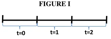
Let us consider an intertemporal equilibrium over three periods 𝑡 = 0,1,2 (see FIGURE I). Production takes place during periods 𝑡 = 0 and 𝑡 = 1, and consumption in periods 𝑡 = 1 and 𝑡 = 2. The possibilities of production are the same as those considered in the stationary framework of the previous section: there are two capital goods, seed corn and iron, produced by means of themselves and labour, and corn is the only consumption good. The methods available for production are those already described in Table 2. Production is considered in gross terms.

FIGURE I

For each of the periods in which production takes place, there is a Master Function that emerges as the result of a maximisation problem of gross corn production. In particular, we have the following problem for the period t=1:

P3: 𝑀𝑎𝑥 𝑄₁ = ∑𝑑_𝑖=𝑎𝑄₁(𝑖)𝑦_𝑖,0

subject to:

∑ 𝐿(𝑖)_𝑦 𝑖,0 𝑔

𝑖=𝑎 = 𝐿0 (P3.1)

∑𝑔𝑖=𝑎𝐾₁(𝑖)𝑦𝑖,0 = 𝐾1,0 (P3.2)

∑𝑔𝑖=𝑎𝐾₂(𝑖)𝑦𝑖,0 = 𝐾2,0 (P3.3)

∑𝑔𝑖=𝑒𝐹₁(𝑖)𝑦𝑖,0 = 𝐹1 (P3.4)

𝑦𝑖,0 ≥ 0, 𝑖 = 𝑎, 𝑏, 𝑐, 𝑑, 𝑒, 𝑓, 𝑔 (P3.5)

where the variable 𝑄_𝑡 is the amount of corn produced in period 𝑡 − 1 and consumed in 𝑡 (e.g. 𝑄₁ is consumed in 𝑡 = 1); 𝑦_𝑖,𝑡 the activity level of method 𝑖 employed in period 𝑡; 𝐿_𝑡 the amount of labour available in period 𝑡; 𝐾_ℎ𝑡 the endowment of the capital good of kind ℎ (i.e. ℎ = 1 for seed corn, ℎ = 2 for iron) available for employment in period 𝑡; and 𝐹_𝑡 the quantity of iron produced in period 𝑡 available for employment one period later (in 𝑡 + 1). Conditions (P3.1)-(P3.3) thus stand for the full-employment of labour and of the endowments of seed corn and iron respectively in period 𝑡 = 1. Condition (P3.4) is instead the market-clearing condition for the iron produced during the first period. Given the non-stationary framework now considered, it may well be the case that the quantity of corn produced during the period is different from the initial endowment of seed corn, i.e.

𝐹1 ≠ 𝐾2,0. Conditions (P3.5) are the usual non-negative constraints imposed on the activity levels 𝑦_𝑖 in the first period.

From P3 it is possible to derive the Master Function MF1 that corresponds to the first period:

𝑄1 = 𝑀𝐹1(𝐿0, 𝐾1,0, 𝐾2,0, 𝐹1) = ∑𝑑𝑖=𝑎𝑄1𝑖𝑦𝑖,0 (15)

Let us now turn to P4, the problem faced in the second period, when there is no production of iron:

P4: 𝑀𝑎𝑥 𝑄₂ = ∑𝑑_𝑖=𝑎𝑄₁𝑖𝑦_𝑖,1

subject to:

∑𝑑𝑖=𝑎𝐿(𝑖)₁ 𝑦𝑖,1 = 𝐿1 (P4.1)

∑𝑑𝑖=𝑎𝐾₁(𝑖)𝑦𝑖,1 = 𝐾1,1 (P4.2)

∑𝑑𝑖=𝑎𝐾₂(𝑖)𝑦𝑖,1 = 𝐾2,1 (P4.3)

𝑦𝑖,1 ≥ 0, 𝑖 = 𝑎, 𝑏, 𝑐, 𝑑 (P4.4)

non-negative constraints on levels of activity. It should be noted that in problem P4 there is no condition analogous to (P3.4). The reason for this should be clear. There is no production in the last period (𝑡 = 2) and therefore no reason to undertake iron production in the previous period (𝑡 = 1), as its consumption in 𝑡 = 2 would be of no benefit to consumers.

The Master Function corresponding to the second period, namely MF2, can be derived from P4:

𝑄2 = 𝑀𝐹2(𝐿0, 𝐾1,1, 𝐾2,1) = ∑𝑖=𝑎𝑑 𝑄1𝑖𝑦𝑖,1 (16)

Now, for the same reasons addressed in the previous sections, it is known that MF1 will be differentiable if exactly four methods at positive levels are employed in the first period, whereas MF2 will be differentiable if there are exactly three methods employed in the second period. As is known, however, this means that exactly four conditions must hold as break-even conditions while three break-even conditions must hold for P4. The remaining conditions will hold as strict inequalities indicating that their employment will not be profitable.

Let us then assume that the solution to P3 is such that methods (𝑐) − (𝑑) − (𝑒) − (𝑓) are employed at positive levels, i.e. 𝑦_𝑖,0 > 0, 𝑖 = 𝑐, 𝑑, 𝑒, 𝑓, and 0 otherwise, while the solution to P4 entails the employment of methods (𝑎) − (𝑏) − (𝑐), i.e. 𝑦_𝑖,1 > 0𝑖 = 𝑎, 𝑏, 𝑐

and 0 otherwise. The differentiability of both MF1 and MF2 requires the following break-even conditions to hold simultaneously:

( ) ( ) ( ) ( )

0 0 1 1,0 2 2,0 1,1

( ) ( ) ( ) ( )

0 0 1 1,0 2 2,0 1,1

( ) ( ) ( ) ( )

0 0 1 1,0 2 2,0 2,1

( ) ( ) ( ) ( )

0 0 1 1,0 2 2,0 2,1 ( ) ( ) ( ) ( ) 1 1 1 1,1 2 2,1 1,2 ( ) ( )

1 1 1 1,1 2

c c c c

d d d d

e e e e

f f f f

a a a c

b b

L w K p K p Q p

L w K p K p Q p

L w K p K p F p

L w K p K p F p

L w K p K p Q p

L w K p K

                 ( ) ( ) 2,1 1,2 ( ) ( ) ( ) ( ) 1 1 1 1,1 2 2,1 1,2

b c

c c c c

p Q p

L w K p K p Q p



  

where 𝑤_𝑡 is for the present value of the wage rate in period 𝑡 and 𝑝_ℎ,𝑡the present value of

commodity ℎ in period 𝑡.

Now, if the value of seed corn is taken as the numéraire, i.e. 𝑝_1,0 = 1, system (17) is a

linear system of seven equations in six unknowns: 𝑤₀, 𝑝_2,0, 𝑤₁, 𝑝_1,1, 𝑝_1,2, 𝑝_2,1. In other words, the system will again be generally overdetermined, with the implication that the marginal products of MF1 and MF2 will again generally not exist. It should be noted, however, that while in the case of the framework examined in the previous section the over-determinacy is due to the fact that the arbitrarily given endowments of capital-goods inputs are incompatible with the stationary conditions there assumed, the intertemporal setting with non-stationary prices is consistent with the arbitrarily given initial endowment. System (17) is overdetermined, however, because the number of methods that must be in use in order for the MF to be differentiable is larger than the number of methods that generally allow the full employment of the initial endowments.

6. Conclusions

Can neoclassical theory dispense with marginal productivity? There is no doubt that Arrow and Debreu’s proof of equilibrium existence is completely independent of it. As for multiplicity and stability, they are issues of such complexity that it is not clear whether the presence of differentiable production functions can be of any help.23 Differentiability is required, however, for local comparative statics, the only kind that can be applied if multiple equilibria cannot be ruled out. Moreover, all the neoclassical theories of growth (both endogenous and exogenous) and most of mainstream macroeconomics derive their results (and policy prescriptions) on the basis of production functions and marginal equalities.

23

The possibility of using these tools is unquestionably important enough to have attracted the attention of one of the most important neoclassical authors, namely Paul Samuelson, the founder of the modern neo-Walrasian approach together with Hicks. Furthermore, he made not just one but two different attempts – following opposite approaches – to justify marginal equalities analytically.

The first was based on the surrogate production function over fifty years ago, when Samuelson tried to obtain a differentiable ‘surrogate’ production function by the aggregation of heterogeneous capital goods into a single input: an amount of ‘jelly’. As pointed out in sections 2 and 3, however, capital goods cannot generally be aggregated without the serious possibility of paradoxical results arising. In particular, further problems arise if the aggregation is performed by using prices, as in Samuelson’s case.

The second is far more recent and instead regards the possibility of having marginal products for the individual capital goods as well as the original inputs. As argued in section 3, if marginal productivity is associated, as is usually the case, with a change in the methods of production in use, then the high degree of specialisation of capital goods makes it impossible to have an economically meaningful marginal product for each of them, because a change in the methods in use entails a change in the kinds of capital goods employed. The attempt made by Samuelson together with Erkko Etula to circumvent this problem therefore consists of basing marginal productivity on the coexistence – rather than change – of different methods of production. While it does not eliminate the need to assume that the different methods employ the same capital goods, the assumption that there is a

continuum of methods that employ the same capital goods in different proportions is considerably weakened, since the MF only assumes the existence of discrete – and comparatively few – methods of production with capital goods in common.

In conclusion, it should be pointed out that above and beyond the problems of the Master Function, the attempt made by Samuelson and Etula as well as all the other contemporary neoclassical efforts that still rely on marginal productivity theory to explain value and distribution are in any case useful because they offer an opportunity to reopen the debate on capital and thus to examine and clarify points that may have been overlooked or inadequately addressed in the existing literature on capital. We hope that this paper has helped to shed at least some faint light on the question.

References

Dantzig, G.B. (1951). “Maximization of a Linear Function of Variables Subject to Linear Inequalities,” in T.C. Koopmans (ed.), Activity Analysis of Production and Allocation. John Wiley & Sons: New York

Etula, E (2006) “The two-sector von Thu¨nen original marginal productivity model of capital; and beyond”; MIT working paper.

Fratini, S. (2007) “Reswitching of techniques in an intertemporal equilibrium model with overlapping generations”; Contributions To political Economy; 26(1): 43-59.

Fratini, S. (2010) “Reswitching and decreasing demand for capital”; Metroeconomica, Vol. 61(4), pp. 676-682.

Fratini, S. (2013a) “Real Wicksell effect, demand for capital and stability”;

Metroeconomica, Vol. 64(2), pp. 346-360.

Fratini, S. (2013b) “Malinvaud on Wicksell’s Legacy to Capital Theory:Some Critical Remarks” in Levrero, S.; Stirati, A.; Palumbo, A. (eds.) Sraffa and the reconstruction of economic theory. Vol. 1. London: McMillan.

Garegnani, P. (1984) “On some illusory instances of marginal products”; Metroeconomica, 36, pp. 143-160.

Garegnani, P. (2007) “'Samuelson's misses: A rejoinder”, The European Journal of the History of Economic Thought, Vol. 14(3), pp. 573 – 585.

Hahn, F. (1975) “Revival of political economy: the wrong issues at the wrong argument”;

Hatta, T. (1976) “The paradox in capital theory and complementarity of inputs”; The Review of Economic Studies, Vol. 43(1), pp. 127-142.

Hicks, J.R. (1932) “Marginal productivity and the principle of variation”, Economica, 35, pp. 79-88.

Malinvaud, E. (1953) “Capital Accumulation and Efficient Allocation of Resources”;

Econometrica, Vol. 21(2), pp. 233-268.

Marx, K. (1909 [1867-1894]) Capital. 3 Vol. Chicago: Charles H. Herr & Company. Pasinetti, L. (1969) “Switches of Technique and the "Rate of Return" in Capital Theory”;

The Economic Journal, Vol. 79(315), pp. 508-531

Robertson, D. (1931), “Wage wrumbles”, in: D.H. Robertson. Economic Fragments. London: P.S. King & Son.

Samuelson, P. A. (1962) “Parable and Realism in Capital Theory: The Surrogate Production Function”; The Review of Economic Studies, Vol. 29(3), pp. 193-206.

Samuelson, P. A. (1966) “A summing-up”; The quarterly journal of economics, Vol. 80 (4), pp. 568-583.

Samuelson, P.A.; Etula, E. (2006) “Complete work-up of the one-sector scalar-capital theory of interest rate: Third installment auditing Sraffa’s never-completed ‘Critique of Modern Economic Theory’’’; Japan and the World economy, Vol. 18, pp. 331-356. Samuelson, P.A. (2007) “Classical and Neoclassical harmonies and dissonances”; The

European Journal of the History of Economic Thought, Vol. 14 (2), 243 - 271

Sraffa, P. (1960) Production of commodities by means of commodities. Prelude to a critique of economic theory; Cambridge: Cambridge University Press.

Swan, T.W. (1956) “Economic growth and capital accumulation”; Economic Record, 32, pp. 334.361.

Trabucchi, P. (2011) “Capital as a Single Magnitude and the Orthodox Theory of Distribution in Some Writings of the Early 1930s”; Review of political economy; Vol. 23(2), pp. 169–188.