Munich Personal RePEc Archive
Heterogeneous Adaptive Expectations
and Coordination in a
Learning-to-Forecast Experiment
Colasante, Annarita and Palestrini, Antonio and Russo,
Alberto and Gallegati, Mauro
Università Politecnica delle Marche
11 September 2015
Online at
https://mpra.ub.uni-muenchen.de/66578/
Heterogeneous Adaptive Expectations and
coordination in a Learning-to-Forecast
Experiment
Annarita Colasante, Antonio Palestrini, Alberto Russo, Mauro Gallegati
Universit`
a Politecnica delle Marche
Preliminary Draft
Abstract
Contents
1 Introduction 3
2 Experimental setting 4
3 Aggregate behavior and emergent heterogeneity 7
4 Why do agents fail to converge to the fundamental value? 15 5 Heterogeneous expectations and coordination in the group 17
6 Final Remarks 21
A General Instruction 32
A.1 Instruction for the forecasting task . . . 32 A.2 Total profits . . . 32
B Tables 32
1
Introduction
The recent financial crisis highlights the strong relation between agents expectations and the real macro and financial variables. The predominant approach in the mainstream literature is based on the Rational Expectation Hypothesis firstly introduced by Muth (1961) and then analyzed in depth by Lucas Jr and Prescott (1971). According to this hypothesis, agents make no systematic errors in their forecasting, taking into account the entire set of available information1.
Experimental evidence suggests that agents form their expectation according to an adaptive rule, that is the forecast is a function of both past expectations and past realizations.
The present work is a contribution in the field of the analysis of agents’ expectation in the experimental financial market. We run a Learning to Forecast Experiment (LtFE) similar to that by Hommeset al. (2005). In this experiment players predict the future price of an asset taking into account the past values of the realized price in the market, the time series of their own past predictions, the mean dividend and the interest rate. Usually, the interest rate and the mean dividend are assumed to be constant. Indeed, the main difference with respect to the existing literature is that we consider a treatment with an increasing fundamental price, in addition to the standard game with a constant fundamental value. Our aim is to investigate individual behavior, and in particular agents’ expectations, in a market with no constant fundamental price. We choose the increasing dividend as a source of market instability to observe if players are able to capture the increasing trend. A recent contribution by Palestrini and Gallegati (2015) shows that, in a context with the value to predict follow a trend and under the hypothesis of adaptive expectations, the individual prediction will be unbiased in the case in which agents are able to estimate the value of the trend.
The growing experimental evidence which deals with the expectation formation should be grouped in two main fields: on the one hand, the approach proposed by Dwyeret al.(1993) in which players predict the future realization of a predefined series, i.e. an Auto Regressive process (Hey (1994)) or a random walk (Bloomfield and Hales (2002)). On the other hand, the method proposed by Marimonet al.(1993) in which the realized price is a function of players’ forecasts. In this field, players should predict the asset price (Hommeset al.(2005), Hommeset al.(2008)) or the price of a commodity (Hommeset al.(2007)). The main difference between these approaches is the role of agents’ expectations. Indeed, only in the LtFE there is an expectation feedback mechanism, that is individual forecasting influences the realized price. For an exhaustive review of these experiment see Assenzaet al.(2014).
We use the Learning-to-Forecast Experiment to analyze not only the forecast ability of players but also the level of coordination in the group. Indeed, we investigate not only the individual expectations but the level of coordination in each group and the link between these variables. This means that players should forecast an endogenous price and, to do so, they must be able to infer the predictions of other participants.
This paper is organized as follows: in Section 2 we describe our experiment and the related works. In Section 3 we show the main graphical results, and in Section 4 and Section 5 we analyze in more detail the level of coordination in a group and the forecasting strategies, respectively.
1
Muth based his analysis on three assumptions: 1) Information is scarce, and the economic system generally does not waste it. 2) The way expectation are formed depends specifically on the structure of the relevant system describing the economy. 3) A “public prediction”, in the sense of Grunberg and Modigliani (1954), will have no substantial effect on the operation of the economic system (unless it is based on inside information). Muth at pg. 317 stresses, in a sense, that the rational expectation hypothesis is made only to represent heterogeneous behaviors of entrepreneurs: “Itdoes notassert that the scratch work of the entrepreneurs resembles the system
2
Experimental setting
The aim of this paper is to understand the mechanism of expectation formation in a financial market with a positive feedback system, that is we assume that the realized price is a function of agents’ expectations. In particular, in a positive feedback system there is a positive correlation between expectations and price, i.e. the higher the forecasting, the higher the price. Financial markets are characterized by this kind of feedback, while the main feature of commodity markets is the negative correlation between predictions and real price.
The existing literature about the analysis of expectation in the lab (see for example Hommes
et al.(2007), Hommeset al.(2008), Heemeijeret al.(2009)) assume that both the mean dividend and the interest rate are constant. The evidence from this stream of literature is that, usually, in the negative feedback system there is a convergence toward the fundamental price, i.e. the equilibrium under the Rational Expectation Hypothesis. This kind of convergence does not occur in the case of positive feedback system, but it has been shown that the coordination among players is faster than that in the negative feedback system. Moreover, Baoet al.(2012) analyze the impact of positive and negative shocks on the price in order to capture the reaction of players and the speed of convergence to the new equilibrium.
The main novelty of the present work is that we consider two different treatments: Treatment 1 in which the mean dividend, and so the fundamental price, is constant over repetition ( ¯d);
Treatment 2 in which the mean dividend increases over time ( ¯dt). Introducing non constant fundamental value increases the uncertainty in the market. Our focus is to investigate the impact of this sources of ambiguity on individual expectations.
We take into account the Asset Price Model, as in Campbell et al. (1997). In this model there is a single security with a dividend dt and a price pt, and a risk-free asset that pays a constant rate R= 1 +runits per period. The dividends are an i.i.d. variable with mean ¯d, so thefundamental price is given bypf = d¯
r.
We run aLearning to Forecast Experiment similar to that proposed by Hommeset al.(2005). The only task of players is to predict the future price of the asset knowing the mean dividend
¯
dand the interest rater. In particular, in the first and in the second period, participants have no information about the past price realizations and about their profit. From the third period, participants are able to see the realized price until periodt−1 and their own forecast. Taking into account these information they must predict the future price of the optionpet+1. In Figure
1 there is the experimental computerized screen. We consider small group of investors, i.e. 6 people, which make their predictions for 51 periods.
Participants to the experiment are divided in groups of six and they receive only qualitative information. Players know that they are advisor of a pension fund and this fund takes into account their predictions to decide how to invest their money between a risk-free asset and a risky option. They do not know the equation that determines the price but they know that the price is given by the equilibrium between demand and supply. Moreover, they know that the higher their prediction the higher the realized price will be. They are informed about the mean dividend and the interest rate. Considering these information, agents could compute, and so predict, the fundamental price.
According to Brock and Hommes (1998), the equation for determining the market price corresponds to the market clearing equilibrium. The theoretical model suggests that each myopic agent, in each period, chooses how much to invest in the risky asset according to the process of maximization of her own future expected wealth. The future wealth (Wt+1) depends on the
Wi,t+1= (1 +r)Wit+zit(pt+1+dt+1−(1−r)pt)
By equating demand, which derives, in turn, from the solution of the problem, and supply we obtain the equilibrium price given by:
pt=
1 1 +r
¯
pet+1+ ¯dt+εt (1)
where ris the interest rate, ¯pe
t+1 is the average predicted price, ¯dtis the mean dividend and
εtis a small normal shock.
Following the same approach in Hommeset al. (2005), we consider in our setting a fraction of computerized fundamentalist computer traders nt. The equation used for the determination of price is the following :
pt=
1 1 +r
h
(1−nt)¯pet+1+ntp f
t + ¯dt+εt i
(2)
where nt is the share of fundamentalist robots in each period. This means that the price is a weighted average between the predicted price by each group and the fundamental price plus a small shock.
The number of robot traders2 is a function of the absolute distance between the realized
market price and the fundamental price. As in Hommes et al. (2005), the equation which determines the share of this trader is defined as:
nt= 1−exp
− 1
200
pt−1−pf
(3)
According to Equation (3), as the price diverges from the fundamental the number of funda-mentalists increases. This mechanism is useful to avoid the creation of bubbles in the market3.
As defined in Hommes (2013), the payoff function depends on the distance between the individual prediction and the realized market price, as in Equation (4):
πit=
1−(pt−p
e it)
2
7
if
pt−peit <7
πit= 0 otherwise
(4)
The experiment involves in total 72 participants (37 female), half of them plays in Treatment 1. In both treatments we considerr= 5%, 6 players in each group and the small shock is such that ε∼N(0,0.25). In Treatment 1 the mean dividend is constant ¯dt and so the fundamental price is equal to pf = 60. In Treatment 2 the mean dividend increases step-by-step by 0.02, so the fundamental price ranges from 60 to 80. The experiment was conducted in October 2014 in the lab of the Faculty of Economics of the Polytechnic University of Marche using the software
z-tree (Fischbacher (2007)). We randomly drawn 72 students in Economics from a population of 390 registered participants sending an invitation email. They were invited to show-up in the Laboratory of Faculty of Economics to participate to the experiment. Each session lasted about
2
According to Assenza et al. (2014), robot fundamentalists are useful to avoid that there is an explosive
increasing of the price. Moreover, since that this kind of traders assert that the deviation from the fundamental price is only temporary, the share of fundamentalists increases with the distance between the realized price and the rational equilibrium.
3
Hommeset al.(2005) run the same experiment with and without the robot traders and they show that there
Table 1: Test of comparison between the realized price and the fundamental value
Treatment 1 Treatment 2
Group t p-value z p-value Groups t p-value z p-value 1 -14.89 <0.01 -13.411 <0.01 1 -41.45 <0.01 -15.079 <0.01 2 -28.23 <0.01 -15.162 <0.01 2 -17.80 <0.01 -13.427 <0.01 3 14.25 <0.01 11.000 <0.01 3 -66.20 <0.01 -15.162 <0.01 4 7.73 <0.01 -6.098 <0.01 4 -56.78 <0.01 -15.162 <0.01 5 27.70 <0.01 14.225 <0.01 5 -43.85 <0.01 -15.162 <0.01 6 42.19 <0.01 14.880 <0.01 6 -73.71 <0.01 -15.162 <0.01
90 minutes and participants were paid by cash at the the end of each session. During the game, prices were expressed in ECU (Experimental Monetary Currency). At the beginning of each session, we read aloud the general instruction and then players read on their screen the specific instructions. The final payment depended on the total gains earned in the game. The mean earning per player was equal to 15 Euro (the exchange rate is 1 Euro = 4 ECU), including the show-up fee4. In Appendix A there are a summary of the instruction and the average payment
per group.
3
Aggregate behavior and emergent heterogeneity
The individual predictions divided in group are shown in Figures 2, 3, 4, 5. On the left panel we observe the realized price with respect to the fundamental value. On the right panel, we show in more detail the individual predictions5.
The main results that emerges from the eye inspection are: i) there is no convergence to the rational expectation equilibrium;ii) in Treatment 2 agents are able to understand that the fundamental value follow an increasing trend;iii)there is heterogeneity both within and between Treatments.
Observing the realized price in each group it is easy to see that all groups converge to a price different to the fundamental value represented by the red line.
According to Hommes (2013), in a positive feedback system we should observe no convergence to the fundamental price but high level of coordination in the group. In order to verify if the difference between the fundamental value and the realized price is statistically significant, we run a t-test and a Wilcoxon test to compare these series. Results are shown in Table 1. Both tests confirm that the realized price for each group is different from the fundamental price, i.e. none of the group converge to the rational expectation equilibrium. In Treatment 1 only Group 2 seems to converge to the fundamental price, that is players behave as if they have rational expectations and in this group there is an high level of coordination. Group 1 reaches an equilibrium close to the fundamental value but there is strong heterogeneity until period 30. Three groups (Group 3, Group 5, Group 6) show a good level of coordination from period 20, but their prediction converge to a price higher than the fundamental. Players in Group 4 coordinate slowly and, at the end, they overestimate the fundamental price6.
4
We give also an extra- bonus to participants who collect perfect prediction in each period.
5
In Figure 3, subfigure (b) and in Figure 4, subfigure (d) we omitted the extreme predictions for a better view of the individual behavior.
6
0
20
40
60
80
100
0 10 20 30 40 50 Period
Fundamental price Realized price
(a) Group 1
55
60
65
20 30 40 50 Period
Sbj 1 Sbj 2 Sbj 3 Sbj 4 Sbj 5 Sbj 6 p_realizzato
(b) Group 1
0
20
40
60
80
100
0 10 20 30 40 50 Period
Fundamental price Realized Price
(c) Group 2
55
60
20 30 40 50 Period
Sbj 1 Sbj 2 Sbj 3 Sbj 4 Sbj 5 Sbj 6 Realized price
(d) Group 2
0
20
40
60
80
100
0 10 20 30 40 50 Period
Fundamental price Realized price
(e) Group 3
60
65
70
20 30 40 50 Period
Sbj 1 Sbj 2 Sbj 3 Sbj 4 Sbj 5 Sbj 6 Realized price
(f) Group 3
0
20
40
60
80
100
0 10 20 30 40 50 Period
Fundamental price Realized price
(a) Group 4
50
55
60
65
70
75
20 30 40 50 Period
Sbj 1 Sbj 2 Sbj 3 Sbj 4 Sbj 5 Sbj 6 Realized price
(b) Group 4
0
20
40
60
80
100
0 10 20 30 40 50 Period
Fundamental price Realized price
(c) Group 5
59
69
79
89
99
20 30 40 50 Period
Sbj 1 Sbj 2 Sbj 3 Sbj 4 Sbj 5 Sbj 6 Realized price
(d) Group 5
0
20
40
60
80
100
0 10 20 30 40 50 Period
Fundamental price Realized price
(e) Group 6
59
69
20 30 40 50 Period
Sbj 1 Sbj 2 Sbj 3 Sbj 4 Sbj 5 Sbj 6 Realized price
[image:10.595.150.448.194.569.2](f) Group 6
0
20
40
60
80
100
0 10 20 30 40 50 Period
Fundamental Price Realized price
(a) Group 1
50
55
60
65
70
20 30 40 50 Period
Sbj 1 Sbj 2 Sbj 3 Sbj 4 Sbj 5 Sbj 6 Realized price
(b) Group 1
0
20
40
60
80
100
0 10 20 30 40 50 Period
Fundamental price Realized price
(c) Group 2
50
60
70
80
90
20 30 40 50 Period
Sbj 1 Sbj 2 Sbj 3 Sbj 4 Sbj 5 Sbj 6 Realized price
(d) Group 2
0
20
40
60
80
100
0 10 20 30 40 50 Period
Fundamental Price Realized price
(e) Group 3
52
57
62
67
72
20 30 40 50 Period
Sbj 1 Sbj 2 Sbj 3 Sbj 4 Sbj 5 Sbj 6 Realized price
[image:11.595.150.448.194.568.2](f) Group 3
0
20
40
60
80
100
0 10 20 30 40 50 Period
Fundamental price Realized price
(a) Group 4
50
60
70
80
20 30 40 50 Period
Sbj 1 Sbj 2 Sbj 3 Sbj 4 Sbj 5 Sbj 6 Realized price
(b) Group 4
0
20
40
60
80
100
0 10 20 30 40 50 Period
Fundamental price Realized price
(c) Group 5
60
65
70
75
20 30 40 50 Period
Sbj 1 Sbj 2 Sbj 3 Sbj 4 Sbj 5 Sbj 6 Realized price
(d) Group 5
0
20
40
60
80
100
0 10 20 30 40 50 Period
Fundamental price Realized price
(e) Group 6
60
70
80
20 30 40 50 Period
Sbj 1 Sbj 2 Sbj 3 Sbj 4 Sbj 5 Sbj 6 Realized price
[image:12.595.150.448.194.568.2](f) Group 6
Table 2: Mean and standard errors of forecasts in Treatment 1
Groups Treatment 1 Treatment 2
Average 1-10 Std.Dev. Average 41-51 Std.Dev. Average 1-10 Std.Dev. Average 41-51 Std.Dev.
1 58.31 9.35 59.19 0.28 55.43 16.91 67.48 1.44
2 57.80 3.42 58.83 0.29 60.71 5.77 68.08 1.70
3 56.65 6.88 65.72 0.57 53.88 7.95 62.96 1.97
4 37.19 12.92 64.57 10.81 47.88 13.95 70.69 3.17
5 59.44 13.81 65.53 1.06 58.36 4.17 73.70 1.20
6 63.65 6.84 64.79 0.62 57.33 3.72 70.74 1.36
In Treatment 2 all the groups underestimate that the fundamental price follow an increasing trend, but all the groups underestimate the magnitude of this trend. In particular, Group 5 and Group 6 show the highest and quickest coordination, and the series of realized prices is very close to the fundamental price. In Group 1, Group 2 and Group 3 there are at least one player which makes odds predictions also after the learning phase, i.e. also after the fifteenth period. Except for these anomalous predictions, it seems that there is a good level of coordination. Also players in Group 4 underestimate the fundamental value, but only for this group the distance between the market price and the fundamental one decreases during repetitions.
The third result is the heterogeneity both within and between Treatments. In each group we observe different behavior, especially at the beginning of the game when players have few information. Starting from the same initial conditions, each group reaches different equilibrium prices as shown in Table 2.
Table 3: Wilcoxon test for multiple comparison among realized price in different groups - Treatment 1
Treatment 1
z p-value z p-value z p-value z p-value z p-value z p-value 1
2 3.075 0.002
3 -6.582 0.000 -6.709 0.000
4 0.157 0.875 0.064 0.949 5.371 0.000
5 -7.352 0.000 -7.379 0.000 -5.893 0.000 -6.877 0.000
6 -8.068 0.000 -8.068 0.000 -5.076 0.000 -7.231 0.000 4.461 0.000
Group 1 2 3 4 5 6
Observing information in Table 2 the heterogeneity between Treatments emerges. First of all, we test if this observed differences are statistically significant. Table 3 and Table 4 report the Wilcoxon test of comparison for each pair of groups. In particular, we compare if the realized price of each group is different from the market price of other groups in the same treatment. With few exceptions, the test confirms the presence of heterogeneity. This result suggests that, since players have the same information to make their forecasting, they predict different prices. Taking into account result in Table 2, also difference in the standard deviation emerges, in particular, the volatility in Treatment 2 is higher than that in the treatment with a constant fundamental price.
Table 4: Wilcoxon test for multiple comparison among realized price in different groups - Treatment 2
Treatment 2
z p-value z p-value z p-value z p-value z p-value z p-value 1
2 -3.229 0.001
3 3.597 0.000 6.408 0.000
4 1.826 0.068 3.832 0.000 0.305 0.761
5 -4.153 0.000 -1.844 0.065 -6.294 0.000 -4.494 0.000
6 -1.938 0.052 0.927 0.354 -5.043 0.000 -3.243 0.001 2.373 0.018
Group 1 2 3 4 5 6
We measure also the level of entropy in each Treatment using the Shannon Entropy index. The index is given by:
S=−
s X
i=1
filnfi (5)
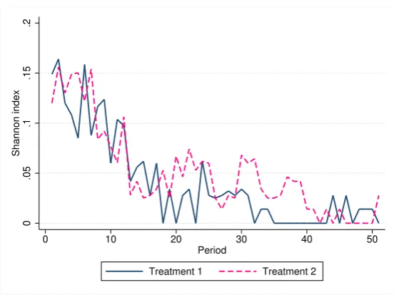
where fi is the relative frequency of the players who make the same forecast. This index is equal to zero in the case of prefect equality of the forecasts. To compute the frequency we split the entire range of the price into windows of width equal to 15. This is a measure of entropy which should be used as a measure of unevenness of the individual predictions within the same Treatment. Figure 6 shows the average standard deviation in each Treatment (blue for Treatment 1 and pink for Treatment 2). As table 2 highlights, the standard deviation is, on average, higher in Treatment 27. Indeed, in Treatment 1 there is a strong reduction of the heterogeneity around
period 5. This means that, since the information about the realized price become available, players quickly coordinate on a common price. In Treatment 2 the high heterogeneity persists until period 15 meaning that players need more time to coordinate in the case of no constant fundamental value.
Looking at the entropy measure shown in Figure 7, similar results emerges. At the beginning of the game there is, on average, the same degree of heterogeneity in both Treatments and, from period 20 on, entropy in Treatment 2 became higher than that in Treatment 1. This means that, since players have few information about past realizations of the price, the entropy is very high in both Treatments. The difference between Treatments emerges after the initial phase of the game, i.e. after period 20, where in Treatment 1 the individual predictions becomes very similar and the index tends to zero. On the other hand, in Treatment 2 the heterogeneity in the forecasts persists after the learning periods highlighting that, in the case of no constant fundamental value, agents find it harder to coordinate their predictions.
Summing up, there is a lack of convergence to the fundamental price in both Treatments and the groups in the same Treatment reach different equilibrium prices, i.e. there is heterogeneity not only between but also within treatments. Comparing the volatility and the entropy in both treatments, a significant difference emerges highlighting that in Treatment 2 the high volatility persists also after the learning phase. This means that, if we introduce a source of instability in the system, i.e. an increasing fundamental price, the volatility increases and the process of convergence takes more time.
7
0
5
10
15
20
Standard deviation
0 10 20 30 40 50
Period
[image:15.595.158.440.131.337.2]Treatment 1 Treatment 2
Figure 6: Average standard deviation of individual forecasts by treatment
0
.05
.1
.15
.2
Shannon index
0 10 20 30 40 50
Period
Treatment 1 Treatment 2
[image:15.595.159.439.429.636.2]Group 1 Group 2 Group 3 Group 4 Group 5 Group 6
0
20
40
60
80
100
Predicted price
1 6 12 18 24 30 36 Subject
(a) Treatment 1
Group 1 Group 2 Group 3 Group 4 Group 5 Group 6
0
20
40
60
80
100
Predicted price
1 7 13 19 25 31 37 Subject
(b) Treatment 2
Figure 8: Individual forecasting in the first period. Different color in each subfigure signals different group. The blue line is the fundamental value.
4
Why do agents fail to converge to the fundamental value?
The REH implies that agents, using all the feasible information, are able to understand the real mechanism of the economy and so they are able to make unbiased forecast. This implies that agents do not need any period for learning or for adapting to a new condition, but, since they know the true behavior of the market, the one step ahead forecasting error is (on average) correct.
In our setting, if all agents have rational expectations, and since that the mean dividend and the interest rate are common knowledge, their predictions should be:
peit=p f
in each period. Within this framework, the possibility that a share of investors has imperfect information, or a lower “degree” or rationality, is ignored on the basis that they would be ruled out - via market selection - by the “smart money” investors, and/or assuming that their impact on aggregate dynamics is negligible (Friedman (1953), Lucas Jr (1978)).
As we said in the previous Section, none of the groups converges to the fundamental price. Why this lack of convergence? There are two main reasons: the first concern the feedback system in the market, the second one deals with individual expectations. Haltiwanger and Waldman (1985) give the definition ofstrategic complements andstrategic substitutes. Individual decisions are strategic complements if agent i has an incentive to play the same strategy of agent j. Conversely, decisions are strategic substitutes if player i has convenience to play the agent j
opposite strategy. Haltiwanger and Waldman (1989) investigate how the market equilibrium, in both the strategic complements and strategic substitutes cases, depends on the interaction between two kind of agents, i.e. sophisticated and naive agents. Sophisticated agents make their forecasting in a rational way, i.e. they are able to compute the fundamental value, while naive agents have adaptive expectations. The conclusion of this investigation is that, taking into account strategic complement decisions, the sophisticated agents are ruled out by naive agents. This implies that, in the case of positive feedback system in which strategies are complements, the convergence to the rational expectation equilibrium does not occur.
dividend. These predictions should be seen as the individual belief of the market price. As we see, there is a share of sophisticated agents that predict the fundamental price. The share of rational agents in Treatment 1 is approximately the 30% and in Treatment 2 this share is equal to 20%. As we observed, the realized price diverges from the fundamental value. This implies that sophisticated agents change their strategy during the game because they have an incentive to follow the strategy played by the majority of agents.
The second explanation for the lack of convergence relies with individual expectations. Ob-serving the graphical results it seems that almost all agents do not use rational expectation to make their prediction, but they probably use some kind of adaptive expectation (Nerlove (1958)). In this case agents look at the past realization of the price (pt) and they try to correct their forecasting (pe
t−1) in each period. The expected price can be written as
pet+1=p
e
t−1+λ(pt−1−p
e
t−1) 0< λ <1
This formulation suggests that agents make systematic forecasting error (pt−pet−1) and,
moreover, they are not able to immediately adjust their expectations. In contrast to the REH, people are backward looking. This implies that agents should underestimate (overestimate) the true value because of this mechanism of correction. Looking at our results, we can conclude that players, on average, adopt some form of adaptive rule. Indeed, especially in Treatment 2, they systematically underestimate the fundamental value. The adaptive expectation hypothesis can be rewritten as a linear combination of past realization and past prediction
pe
t+1=λpt−1+ (1−λ)p
e
t−1 (6)
The formulation in Equation (6) is the simplest form of adaptive expectation. According to our graphical results, agents in our game use some kind of adaptive expectation since they systematically underestimate or overestimate the fundamental value. Following an approach similar to Baoet al.(2012), we estimate the following equation for each agent:
pet+1=α0+
k X
i=1
αipt−i+ q X
j=0
βjpet−j+εt (7)
This is an Autoregressive Distributed Lag (ADL(k,q)). We estimate different models with different lags and we choose an ADL(4,4), i.e. a model in which we consider four lags of the dependent variable and four lags of the realized price, taking into account the information criteria (AIC, BIC), the presence of serial correlation in the residuals8 and we test the stationarity
condition.
Results are shown in the Appendix in Tables 13-18 for the six groups in Treatment 1, and in Tables 19-24 for groups in Treatment 2. Each column refers to a single agent. For each individual we report the estimated coefficients αi and βj, the standard error, the R-squared of the regression, the presence of serial correlation9, the Phillips-Perron unit root test and the
estimate prediction strategy. We categorize players as “ADAPTIVE” when both αi and βj coefficients are significant. “AR(q)” refers to expectations based on the past value of the realized price, i.e. those estimation for which only coefficientsαiare significant. We classify as “NAIVE” agents which show onlyα1as a significant coefficient. There are also some individuals for which
only some of the coefficientsβj are significant and we classify them as “OBSTINATE”.
8
See Tables 9-10 for the information criteria and Tables 11-12 for the p-value of the Breusch-Godfrey test. We choose the specification for which both the information criteria and the correlation are minimum.
9
Looking at these results it is easy to see that there is heterogeneity in the agents’ behavior both within and between groups10.
In Treatment 1 the following evidence emerges:
• Group 1 and Group 2 show similar pattern of the realized price, but players have hetero-geneous expectations. The common features of these groups is that players update their set of available information also with past realizations, i.e. αi coefficients with i > 1 are strongly significant.
• Group 3, Group 5 and Group 6 show similar pattern. Indeed, most of them take into account only the first lag of the realized price, i.e. the last value they are able to see in the game, and the first lag of their own expectation. Since they consider only recent infor-mation, and since there are some players that show “obstinate” behavior. they coordinate to a price higher than the fundamental from the early periods and they are not able to correct their forecasting errors with respect to the fundamental price.
• Players in Group 4 behave as if they are myopic, and such behavior leads to a persistent volatility through all the game11.
Results for Treatment 2 can be summarized as follows:
• the majority of players in Group 1, Group 3 and Group 4 have adaptive expectations. In particular, to form their expectation agents take into account especially past realizations of their own expectations.
• in Group 2 and Group 5 there is a large share of players with obstinate behavior. More in general in these groups players consider only recent information to make their forecasts.
• in Group 6 players have heterogeneity expectations but many of them assign an high weight to past information.
From the analysis of the individual expectations we find out three main results: - the lack of convergence to the fundamental price is due to the fact that the majority of players have adaptive expectations; - the observed heterogeneity within Treatments depends on the heterogeneity of agents’ expectations; - there are no significant difference in the expectation formation between Treatments, i.e. the majority of players form their expectation using an adaptive rule also in the case of increasing fundamental value. Since agents have adaptive expectations in both Treat-ments, in Treatment 2 players take into account past information to make their forecasts. This means that agents use recent information to understand the current price and past information to extrapolate the trend.
5
Heterogeneous expectations and coordination in the group
In this Section we analyze the level of coordination in each group. We compute theindividual average forecast error to analyze the level of coordination within groups as in Hommes et al.
(2008). The average forecast error is the quadratic difference between the individual prediction and the realized price. This error should be decomposed into two parts:
10
Our estimation fails to predict the behavior of 8 agents since there is autocorrelation in the residual.
11
Table 5: Average quadratic errors from market price in Treatment 1
Groups Average individual error Average dispersion Average common error
1
N T PN
i=1
PT
t=15(peit−pt)2 N T1 PN
i=1
PT
t=15(peit−p¯t)2 T1 PT
t=15(¯pet−pt)2
1 0.38 0.29(76%) 0.09(24%)
2 0.16 0.06(41%) 0.09(59%)
3 0.80 0.59(73%) 0.21(27%)
4 50.27 50.10(99%) 0.17(1%)
5 2.12 1.21(57%) 0.91(43%)
6 0.72 0.42(57%) 0.31(43%)
Table 6: Average quadratic errors from market price in Treatment 2
Groups Average individual error Average dispersion Average common error
1
N T PN
i=1
PT
t=15(peit−pt)2 N T1 PN
i=1
PT
t=15(peit−p¯t)2 T1 PT
t=15(¯pet−pt)2
1 1.76 0.98(56%) 0.79(44%)
2 40.49 39.81(98%) 0.68(2%)
3 4.48 2.47(55%) 2.01(45%)
4 4.21 3.19(76%) 1.02(24%)
5 0.42 0.30(72%) 0.12(28%)
6 0.54 0.21(39%) 0.33(61%)
1
N T 51
X
t=t0
6
X
i=1
(peit−pt)2= 1
N T 51
X
t=t0
6
X
i=1
(peit−p¯ e t)2+ 1
T 51
X
t=t0
(¯pet−pt)2 (8)
The term 1
N T P51
t=t0
P6
i=1(peit−p¯et)2 is the average dispersion error, that is the distance between the individual prediction and the average prediction of the group. The second term
1
T P51
t=t0(¯p
e
t−pt)2is theaverage common error, that is the measure of the distance between the average prediction of the group and the realized price. We take into account the observation starting fromt0= 15. Results are shown in Table 5 and Table 6.
Group 2 (Treatment 1) and Group 6 (Treatment 2) are those with the best coordination in the sense that they show not only low value of the individual average forecasting errors but also an high value of the average common error. Figure 9 shows a summary of the prediction rules adopted in each group. As we point out in the previous Section, the majority of players form their expectations following an adaptive rule, especially in Treatment 2.
If we take a look at the players expectations in Group 2 (treatment 1) and Group 6 (Treatment 2) in Figure 9, it is easy to see that Players in Group 2 have homogeneous expectations, while this is not the case for Group 6. This implies that the homogeneity of expectations is not a sufficient condition to have a good level of coordination.
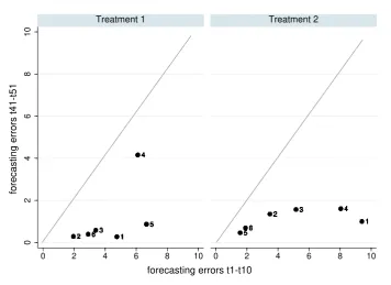
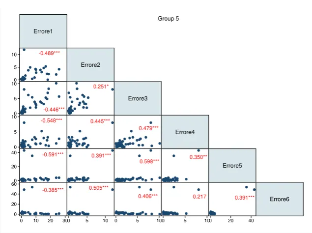
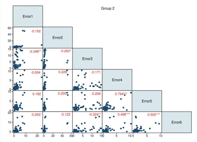
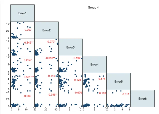
What are the reasons behind these different level of coordination? First of all, the high level of coordination derives from a process of learning of others’ expectations. One of the measure we take into account is the relation between the average forecasting error at the beginning and at the end of the game. If there is a learning process, or more generally a process of convergence to a specific equilibrium, there should be a reduction of the forecasting error from the beginning to the end of the game. Figure 10 shows the relation between the forecasting errors at the beginning of the game and these errors at the end of the game. At a glance, there is a learning process for all groups since the point lies under the bisector. This implies that the forecasting accuracy is better at the end of the game meaning that players have learned how to coordinate. Group 1 in Treatment 2 shows the best learning process, indeed, the average error at the beginning is equal to 10 and they are able to reduce this value up to 2 by the end of the game. Group 2 in Treatment 1 and Group 5 and Group 6 in Treatment 2 are those with the lowest average forecasting error from the beginning and their errors become close to zero at the end of the game. Although some groups show a strong reduction of their forecasting errors, they do not reach a good level of coordination. To better understand why this happens, we compute the contemporaneous correlation of the forecasting errors for each pair of subjects in the same group. Figures 12- 17 and Figure 18-23 show the scatter plot and the value of the correlation between the individual forecasting errors in each group for each pair of players. Focusing on Figure 13 and Figure 23, i.e. correlation in the groups with the best level of coordination, we find out that significant correlations are always positive. This means that players co-move in the same direction in each period and thus they are able to capture the others’ prediction strategy during the whole game. The other factor that influences the level of coordination is linked to the heterogeneity of players’ initial belief. In the previous Section we have seen that individual predictions in the first period are quite different (see Figure 8). Using Equation (5) we compute the Shannon entropy index for the individual forecasts in each group. Results in Figure 11 suggest that in some groups the level of heterogeneity is high until the end of the game. Taking a look at Group 2 (Treatment 1) and Group 6 (Treatment 2) an interesting feature emerges. For those groups the entropy index is equal to zero in the first period. Also in Group 5 in Treatment 2 the level of heterogeneity is close to zero at the beginning of the game and this Group shows a good level of coordination very similar to Group 6 in the same Treatment.
Merging the results, we find out that groups in which players have homogeneous expectations do not show the same level of coordination. This implies that the ability to coordinate depends on other factors. We analyze in depth the individual forecasting errors and we conclude that the level of coordination is better if the errors are positively correlated. Moreover, we point out the importance of the initial conditions, i.e. groups with low entropy at the beginning of the game are able to reach a good level of coordination in a few periods.
Group 1 Group 2 Group 3
Group 4 Group 5 Group 6
AR Adaptive Naive None Obstinate
(a) Treatment 1
Group 1 Group 2 Group 3
Group 4 Group 5 Group 6
AR Adaptive Naive None Obstinate
(b) Treatment 2
1 1 1 1 1 1 1 1 1 1 1 1 1 1 1 1 1 1 1 1 1 1 1 1 1 1 1 1 1 1 1 1 1 1 1 1 1 1 1 1 1 1 1 1 1 1 1 1 1 1 1 1 1 1 1 1 1 1 1 1 1 1 1 1 1 1 2 2 2 2 2 2 2 2 2 2 2 2 2 2 2 2 2 2 2 2 2 2 2 2 2 2 2 2 2 2 2 2 2 2 2 2 2 2 2 2 2 2 2 2 2 2 2 2 2 2 2 2 2 2 2 2 2 2 2 2 2 2 2 2 2 2 333333333333333333333333333333333333333333333333333333333333333333
4 4 4 4 4 4 4 4 4 4 4 4 4 4 4 4 4 4 4 4 4 4 4 4 4 4 4 4 4 4 4 4 4 4 4 4 4 4 4 4 4 4 4 4 4 4 4 4 4 4 4 4 4 4 4 4 4 4 4 4 4 4 4 4 4 4 5 5 5 5 5 5 5 5 5 5 5 5 5 5 5 5 5 5 5 5 5 5 5 5 5 5 5 5 5 5 5 5 5 5 5 5 5 5 5 5 5 5 5 5 5 5 5 5 5 5 5 5 5 5 5 5 5 5 5 5 5 5 5 5 5 5 6 6 6 6 6 6 6 6 6 6 6 6 6 6 6 6 6 6 6 6 6 6 6 6 6 6 6 6 6 6 6 6 6 6 6 6 6 6 6 6 6 6 6 6 6 6 6 6 6 6 6 6 6 6 6 6 6 6 6 6 6 6 6 6 6 6 1 1 1 1 1 1 1 1 1 1 1 1 1 1 1 1 1 1 1 1 1 1 1 1 1 1 1 1 1 1 1 1 1 1 1 1 1 1 1 1 1 1 1 1 1 1 1 1 1 1 1 1 1 1 1 1 1 1 1 1 1 1 1 1 1 1 2 2 2 2 2 2 2 2 2 2 2 2 2 2 2 2 2 2 2 2 2 2 2 2 2 2 2 2 2 2 2 2 2 2 2 2 2 2 2 2 2 2 2 2 2 2 2 2 2 2 2 2 2 2 2 2 2 2 2 2 2 2 2 2 2
2 333333333333333333333333333333333333333333333333333333333333333333 444444444444444444444444444444444444444444444444444444444444444444 5 5 5 5 5 5 5 5 5 5 5 5 5 5 5 5 5 5 5 5 5 5 5 5 5 5 5 5 5 5 5 5 5 5 5 5 5 5 5 5 5 5 5 5 5 5 5 5 5 5 5 5 5 5 5 5 5 5 5 5 5 5 5 5 5 5666666666666666666666666666666666666666666666666666666666666666666
0 2 4 6 8 10
0 2 4 6 8 10 0 2 4 6 8 10
Treatment 1 Treatment 2
forecasting errors t41-t51
[image:22.595.120.477.100.359.2]forecasting errors t1-t10
Figure 10: Relation between average forecasting errors at the beginning and at the end of the game.
that a certain degree of heterogeneity is necessary to have a stability in the system. Indeed, in this Section we have shown that, since players have heterogeneous expectations, it is possible to reach a stable, not rational equilibrium if agents are able to coordinate with each other.
6
Final Remarks
In this work we investigate the individual behavior in an experimental asset market in which participants play in groups of six. In this market players see the mean dividend and the interest rate which are common knowledge for all groups. Moreover, during the game each individual observes the past realization of the market price and her own past predictions. Using all the feasible information, agents in each period make a two-periods ahead forecast of the asset price. The realized price is a function of the average forecasting of the group. The fundamental price is given by the ratio between the mean dividend and the interest rate. We run two treatments in which the only difference is the process which generates the fundamental price: in Treatment 1 both the mean dividend and the interest rate are constant, while in Treatment 2 the mean dividend is increasing during repetitions.
0.167
0
0.151
0.204
0.167 0.204
0
.1
.2
.3
.4
.5
0
.1
.2
.3
.4
.5
0 20 40 60 0 20 40 60 0 20 40 60
Group 1 Group 2 Group 3
Group 4 Group 5 Group 6
Shannon Entropy index
Period
(a) Treatment 1
0.151 0.167 0.151
0.167
0.085
0
0
.1
.2
.3
.4
.5
0
.1
.2
.3
.4
.5
0 20 40 60 0 20 40 60 0 20 40 60
Group 1 Group 2 Group 3
Group 4 Group 5 Group 6
Shannon Entropy index
Period
(b) Treatment 2
0.085
0.245* 0.047
-0.301** 0.105 -0.275*
0.048 0.267* 0.185 -0.346
-0.098
-0.059 -0.029 0.267*
-0.175
Error1
Error2
Error3
Error4
Error5
Error6
0 10 20 30 0
2 4 6
0 2 4 6 0
10 20 30
0 10 20 30 0
2 4 6
0 2 4 6 0
5 10
0 5 10 0
20 40
Group 1
Figure 12: Correlation of individual forecasting errors
0.084
0.000 0.369***
0.329**
0.563***
0.322**
0.262 -0.016 0.290** 0.311**
0.056 0.397*** 0.563*** 0.428*** -0.452***
Error1
Error2
Error3
Error4
Error5
Error6
0 2 4 6 0
5 10
0 5 10 0
2 4 6
0 2 4 6 0
2 4
0 2 4 0
1 2 3
0 1 2 3 0
5 10
Group 2
0.044
0.198 -0.17
0.042 0.203 0.112
-0.087 0.094 -0.175 -0.436***
0.166 -0.001 0.033 -0.041 0.123
Error1
Error2
Error3
Error4
Error5
Error6
0 5 10 0
2 4
0 2 4 0
2 4 6
0 2 4 6 0
5 10
0 5 10 0
10 20
0 10 20 0
5 10
Group 3
Figure 14: Correlation of individual forecasting errors
0.18
0.258*
0.425***
0.354** 0.418*** 0.087
-0.246* -0.089 -0.352** -0.127
0.135 0.403*** 0.459*** 0.403** -0.321**
Errore1
Errore2
Errore3
Errore4
Errore5
Errore6
0 10 20 0
5 10 15
0 5 10 15 0
20 40
0 20 40 0
10 20 30
0 10 20 30 0
20 40 60
0 20 40 60 0
20 40
Group4
-0.489***
-0.446***
0.251*
-0.548*** 0.445***
0.479***
-0.591*** 0.391***
0.598*** 0.350**
-0.385*** 0.505***
0.406*** 0.217 0.391***
Errore1
Errore2
Errore3
Errore4
Errore5
Errore6
0 10 20 30 0
5 10
0 5 10 0
5 10
0 5 10 0
5 10
0 5 10 0
20 40
0 20 40 0
20 40 60
Group 5
Figure 16: Correlation of individual forecasting errors
0.514***
0.178 0.173
0.093 0.233* -0.207
-0.112 -0.001 -0.118 0.295**
-0.082 -0.166 -0.293** -0.188 -0.267*
Error1
Error2
Error3
Error4
Error5
Error6
0 2 4 0
5 10 15
0 5 10 15 0
2 4 6
0 2 4 6 0
10 20
0 10 20 0
5 10
0 5 10 0
2 4 6
[image:26.595.139.457.114.351.2]Group 6
0.531***
0.162 0.289**
-0.369*** -0.396***
-0.413***
0.046
0.168
0.415***
-0.512***
0.326*
0.262* -0.396***
-0.376***
0.168
Error1
Error2
Error3
Error4
Error5
Error6
0 5 10 15 0
5 10
0 5 10 0
10 20
0 10 20 0
20 40 60
0 20 40 60 0
10 20
0 10 20 0
10 20
[image:27.595.140.458.115.352.2]Group 1
Figure 18: Correlation of individual forecasting errors
-0.152
-0.348** -0.263*
-0.004 0.229 -0.171
0.182 0.200 -0.206 0.794***
0.255* -0.122 -0.324** 0.496*** 0.505***
Error1
Error2
Error3
Error4
Error5
Error6
0 10 20 0
20 40 60
0 20 40 60 0
5 10 15
0 5 10 15 0
5 10
0 5 10 0
5 10
0 5 10 0
10 20
Group 2
[image:27.595.138.457.418.647.2]0.356***
0.222 0.024
0.185 -0.103 -0.015
-0.626*** -0.347** -0.510*** -0.265*
0.535*** -0.010 -0.024 -0.038 -0.313**
Error1
Error2
Error3
Error4
Error5
Error6
0 5 10 15 0
5 10
0 5 10 0
5 10 15
0 5 10 15 0
5 10
0 5 10 0
10 20
0 10 20 0
5 10
[image:28.595.139.457.114.351.2]Group 3
Figure 20: Correlation of individual forecasting errors
-0.207
0.342** -0.270*
0.254* -0.318** 0.192
0.581*** -0.115
0.128 0.174
-0.082
-0.070
-0.346** 0.199 -0.011
Error1
Error2
Error3
Error4
Error5
Error6
0 5 10 15 0
20 40
0 20 40 0
5 10
0 5 10 0
5 10
0 5 10 0
2 4 6
0 2 4 6 0
20 40
Group 4
[image:28.595.138.457.418.646.2]0.207
0.301** 0.173
0.349** 0.265*
0.224
0.198 -0.075 -0.009 0.083
0.216 0.155 0.189 0.438*** 0.086
Error1
Error2
Error3
Error4
Error5
Error6
0 1 2 0
5 10 15
0 5 10 15 0
5 10
0 5 10 0
2 4 6
0 2 4 6 0
1 2 3
0 1 2 3 0
1 2
[image:29.595.138.457.114.351.2]Group 5
Figure 22: Correlation of individual forecasting errors
-0.247*
0.434*** 0.008
0.122 0.091 0.306**
0.506*** 0.216 0.523*** 0.270*
-0.209 0.300** -0.177 0.277** 0.132
Error1
Error2
Error3
Error4
Error5
Error6
0 5 0
2 4 6
0 2 4 6 0
2 4 6
0 2 4 6 0
2 4 6
0 2 4 6 0
1 2 3
0 1 2 3 0
2 4 6
Group 6
[image:29.595.139.457.418.647.2]individual predictions. This kind of ADL(k,q) model fits very well the behavior of almost all agents. What emerges is that the majority of players form their expectations using an adaptive rule. Comparing the individual expectations in both Treatments, even if agentsin Treatment 2 weight more past information, no significant different emerges.
From the analysis of the individual forecasting errors emerges that groups have different level of coordination. The key result we find out is that the homogeneity of expectations in the same group is not a sufficient condition to have a strong coordination. Analyze the correlation between agents’ forecasting errors,
The analysis of the correlation between individual forecasting errors highlights that a positive and significant correlation of these errors leads to a good level of coordination. Finally, we find out that a low level of entropy at the beginning of the game strongly influence the coordination in each group.
References
Assenza, T., Bao, T., Hommes, C., and Massaro, D. (2014). Experiments on expectations in macroeconomics and finance. InExperiments in macroeconomics, pages 11–70. Emerald Group Publishing Limited.
Bao, T., Hommes, C., Sonnemans, J., and Tuinstra, J. (2012). Individual expectations, limited rationality and aggregate outcomes.Journal of Economic Dynamics and Control,36(8), 1101– 1120.
Bloomfield, R. and Hales, J. (2002). Predicting the next step of a random walk: experimental evidence of regime-shifting beliefs. Journal of financial Economics,65(3), 397–414.
Brock, W. A. and Hommes, C. H. (1998). Heterogeneous beliefs and routes to chaos in a simple asset pricing model. Journal of Economic dynamics and Control,22(8-9), 1235–1274. Campbell, J. Y., Lo, A. W.-C., MacKinlay, A. C., et al.(1997). The econometrics of financial
markets, volume 2. princeton University press Princeton, NJ.
Dwyer, G. P., Williams, A. W., Battalio, R. C., and Mason, T. I. (1993). Tests of rational expectations in a stark setting. The Economic Journal, pages 586–601.
Fischbacher, U. (2007). z-tree: Zurich toolbox for ready-made economic experiments. Experi-mental Economics,10(2).
Friedman, M. (1953). Essays in positive economics. University of Chicago Press.
Grunberg, E. and Modigliani, F. (1954). The predictability of social events. The Journal of Political Economy, pages 465–478.
Haltiwanger, J. and Waldman, M. (1985). Rational expectations and the limits of rationality: An analysis of heterogeneity. The American Economic Review, pages 326–340.
Haltiwanger, J. and Waldman, M. (1989). Limited rationality and strategic complements: the implications for macroeconomics. The Quarterly Journal of Economics, pages 463–483. Heemeijer, P., Hommes, C., Sonnemans, J., and Tuinstra, J. (2009). Price stability and volatility
in markets with positive and negative expectations feedback: An experimental investigation.
Journal of Economic dynamics and control,33(5), 1052–1072.
Hey, J. D. (1994). Expectations formation: Rational or adaptive or...? Journal of Economic Behavior & Organization,25(3), 329–349.
Hommes, C. (2011). The heterogeneous expectations hypothesis: Some evidence from the lab.
Journal of Economic Dynamics and Control,35(1), 1–24.
Hommes, C. (2013). Behavioral rationality and heterogeneous expectations in complex economic systems. Cambridge University Press.
Hommes, C., Sonnemans, J., Tuinstra, J., and Van de Velden, H. (2005). Coordination of expectations in asset pricing experiments. Review of Financial Studies, 18(3), 955–980. Hommes, C., Sonnemans, J., Tuinstra, J., and Van De Velden, H. (2007). Learning in cobweb
Hommes, C., Sonnemans, J., Tuinstra, J., and van de Velden, H. (2008). Expectations and bubbles in asset pricing experiments. Journal of Economic Behavior & Organization, 67(1), 116–133.
Kirman, A. (2006). Heterogeneity in economics. Journal of Economic Interaction and Coordi-nation,1(1), 89–117.
Kirman, A. P. (1992). Whom or what does the representative individual represent? The Journal of Economic Perspectives, pages 117–136.
Lucas Jr, R. E. (1978). Asset prices in an exchange economy. Econometrica: Journal of the Econometric Society, pages 1429–1445.
Lucas Jr, R. E. and Prescott, E. C. (1971). Investment under uncertainty.Econometrica: Journal of the Econometric Society, pages 659–681.
Marimon, R., Spear, S. E., and Sunder, S. (1993). Expectationally driven market volatility: an experimental study. Journal of Economic Theory,61(1), 74–103.
Muth, J. F. (1961). Rational expectations and the theory of price movements. Econometrica: Journal of the Econometric Society, pages 315–335.
Nerlove, M. (1958). Adaptive expectations and cobweb phenomena. The Quarterly Journal of Economics, pages 227–240.
A
General Instruction
You are a financial advisor to a pension fund that wants to invest an amount of money to buy an asset. The pension fund will allocate its money between a bank account which pays fix interest and a risky investment. The allocation depends on you forecast accuracy. Your task is to predict the price of the risky asset for 51 periods. Your profit depends on your forecast accuracy. The better your prediction, the higher the profit in each period. The final earning will be given by the sum of the profit you gain in each period.
A.1
Instruction for the forecasting task
At the beginning of each period you must predict the price for the next period, i.e. in period 1 you must predict the price of period 2 and so on. At the beginning of the experiment you should predict the price of the first and the second period. You forecasting for these period must be between 0 and 100. To make these predictions you will have only two information: the mean dividend and the interest rate. From period 3 until the end of the game you will have more information12: besides the interest rate and the mean dividend, you will see a graph with the
time series of your past prediction and the series of the realized price in the market. The green dots represent the series of the predicted price, while the blue dots represents the realized price in each period. Moreover, you will see the values of these series.
At period t the feasible information will be: the realized price up to periodt−2, your past prediction up to periodt−1 and your earning up to periodt−2.
Once each players have made their prediction for the first and the second period, the realized price in period 1 and your prediction in period 1 and period 2 will be revealed. The same mechanism holds for subsequent periods. After you insert the forecasting your profit will be computed according to the forecasting accuracy. In each period your profit ranges between 0 (bad forecast) and 1 (best forecast). During the experiment your earning will be expressed in ECU (Experimental Currency Unit) and at the end of the game the amount will be converted in Euro (1 ECU = 0.4 Euro).
The market price will be determined by the equilibrium between demand and supply of the stock. The supply of stocks is fixed for the duration of the experiment. The demand of stocks will be given by the aggregate demand of each pension fund of which each participant is the advisor.
A.2
Total profits
Table 7 shows the total profit in Euro in each group. Table 8 reports the descriptive statistics of the cash earned in both treatments.
B
Tables
C
Estimation of individual prediction rules
12
Table 7: Average payment by group
Treatment 1 Treatment 2
Group 1 88.80 78.09
Group 2 110.07 86.08
Group 3 88.17 93.34
Group 4 77.81 80.56
Group 5 82.70 100.48
[image:34.595.207.387.222.316.2]Group 6 105.84 101.49
Table 8: Descriptive statistics of payment
Mean Std. Dev Min Max
Treatment 1 15.37 12.89 11.68 25.59
Table 9: Information Criteria - Treatment 1
ADL(1, 1) ADL(2,2) ADL(3,3) ADL(4,4)
Subject AIC BIC AIC BIC AIC BIC AIC BIC
1 220.76 226.44 190.52 199.88 172.73 185.67747 141.42 157.88
2 120.61 126.28 112.1 121.46 95.601 108.55234 53.36 69.818
3 181.35 187.02 157.88 167.23 146.65 159.60119 128 144.46
4 189.38 195.05 170.01 179.37 168.6 181.54864 161.05 177.5
5 169.75 175.42 112.38 121.73 68.014 80.965353 67.321 83.779
6 118.76 124.43 106.02 115.38 71.099 84.049693 53.788 70.246
7 143.85 149.52 126.78 136.13 115.53 128.48259 95.634 112.09
8 115.72 121.4 50.217 59.573 23.058 36.009119 -51.52 -35.06
9 42.009 47.685 23.465 32.821 2.2757 15.226693 -36.05 -19.6
10 109.33 115 27.328 36.684 -18.93 -5.9787253 -16.55 -0.094
11 121.07 126.74 64.07 73.426 58.724 71.675155 44.58 61.038
12 49.255 54.931 -9.869 -0.513 -19.04 -6.0853933 -44.46 -28
13 174.29 179.96 99.431 108.79 96.31 109.26108 80.552 97.01
14 92.474 98.149 82.933 92.289 71.048 83.9986 62.177 78.635
15 153.68 159.36 152.95 162.31 136.69 149.64194 127.35 143.81
16 200.86 206.53 182.11 191.46 171.42 184.37051 162.37 178.83
17 212.7 218.38 202.12 211.48 168.4 181.34658 156.23 172.69
18 133.98 139.66 103.76 113.11 87.569 100.52042 89.845 106.3
19 239.67 245.35 222.68 232.03 221.96 234.90779 220.56 237.02
20 244.22 249.9 238.33 247.69 236.3 249.24763 220.24 236.7
21 175.93 181.6 173.57 182.93 164.01 176.96593 164.14 180.6
22 229.68 235.36 225.76 235.12 201.78 214.72791 195.09 211.55
23 409.81 415.48 404.79 414.14 399.26 412.20644 390.34 406.8
24 195.09 200.77 189.54 198.9 185.92 198.86695 156.28 172.74
25 312.69 318.36 307.95 317.31 303.71 316.65889 300.92 317.38
26 141.55 147.23 115.28 124.64 107.3 120.24928 104.76 121.21
27 183.08 188.75 139.08 148.43 114.49 127.43721 116.23 132.69
28 164.63 170.3 165.62 174.97 163.54 176.48715 161.52 177.97
29 163.71 169.39 154.71 164.06 145.2 158.15401 145.76 162.22
30 72.255 77.931 65.253 74.609 68.735 81.685607 72.497 88.954
31 128.47 134.15 115.15 124.51 68.446 81.397446 65.882 82.34
32 103.8 109.48 98.224 107.58 54.847 67.797679 54.188 70.646
33 140.37 146.05 125.52 134.88 91.228 104.17953 79.782 96.24
34 116.74 122.42 104.75 114.11 94.981 107.93219 92.312 108.77
35 113.94 119.62 80.678 90.034 64.321 77.271674 67.736 84.194
Table 10: Information Criteria - Treatment 2
ADL(1, 1) ADL(2,2) ADL(3,3) ADL(4,4)
Subject AIC BIC AIC BIC AIC BIC AIC BIC
1 225.93 231.61 199.1 208.46 220.03012 232.98 204.6 221.05
2 207.17 212.85 152.69 162.05 177.66975 190.62 176.53 192.99
3 180.45 186.13 408.2 417.56 126.87811 139.83 114.68 131.14
4 416.61 422.29 214.12 223.47 377.31744 390.27 357.19 373.64
5 265.88 271.55 205.32 214.68 213.12688 226.08 210.71 227.16
6 217.86 223.53 276.02 285.37 184.21299 197.16 177.74 194.2
7 279.74 285.42 367.12 376.47 236.00816 248.96 234.54 250.99
8 373.57 379.25 301.15 310.5 361.7466 374.7 357.66 374.12
9 306.58 312.26 185.15 194.51 296.55492 309.51 293.45 309.9
10 205.44 211.11 77.517 86.873 148.00698 160.96 111.31 127.76
11 105.89 111.57 168.02 177.37 73.267574 86.219 74.987 91.444
12 186.25 191.93 109.39 118.75 161.96718 174.92 153.08 169.53
13 129.39 135.07 203.86 213.22 79.706817 92.658 75.76 92.218
14 230.81 236.48 238.26 247.61 169.03668 181.99 158.96 175.42
15 244.18 249.86 93.646 103 220.84647 233.8 179.91 196.37
16 99.369 105.04 255.37 264.72 87.686376 100.64 78.829 95.286
17 283.52 289.2 145.89 155.25 224.69208 237.64 224.59 241.05
18 148.93 154.61 116.23 125.59 137.98534 150.94 83.478 99.935
19 161.4 167.08 354.5 363.85 108.43299 121.38 107.76 124.22
20 360.35 366.02 191.71 201.07 349.8425 362.79 343.41 359.87
21 194.28 199.95 187.77 197.12 182.82506 195.78 182.47 198.93
22 196.96 202.64 184.73 194.09 174.63629 187.59 161.66 178.12
23 205.13 210.81 230.07 239.42 164.16166 177.11 123.56 140.02
24 317.71 323.38 49.983 59.339 214.47617 227.43 206.2 222.66
25 89.439 95.114 -23.81 -14.46 31.759689 44.711 34.191 50.649
26 28.847 34.522 85.505 94.861 -32.622354 -19.67 -30 -13.54
27 164.73 170.41 73.463 82.819 48.590901 61.542 42.448 58.906
28 125.44 131.12 109.1 118.46 47.044476 59.996 15.375 31.833
29 126.54 132.21 36.242 45.598 81.114647 94.066 47.566 64.024
30 59.963 65.638 73.177 82.533 28.20435 41.155 28.724 45.181
31 75.258 80.933 97.43 106.79 60.127071 73.078 57.943 74.4
32 149.27 154.94 54.815 64.171 93.639318 106.59 90.136 106.59
33 68.047 73.722 153.06 162.42 44.744136 57.695 48.154 64.611
34 163.67 169.34 9.8552 19.211 135.5598 148.51 78.858 95.316
35 18.267 23.943 3.9161 13.272 -2.8625397 10.088 2.4225 18.88
Table 11: Breush-Godfrey test for autocorrelation up to 20 lags - Treatment 1
ADL(1.1) ADL(2.2) ADL(3.3) ADL(4.4)
.04497221 .70740166 .06906673 .61693958 .35248651 .00754329 .00160015 .25696191 .34784263 .04215838 .32996119 .19720005
.5747241 .34634766 .69367723 .52779671
.7450133 .21808757 .41504783 .38485453
.14885972 .27450356 .598198 .29070712
.26131274 .07026125 .13641375 .57469519
.4958191 .53949361 .06115906 .7182538
.08629488 .10585359 .16861862 .21212992 .00089042 .90404816 .81164251 .43167646 .51644267 .68276758 .19013669 .01072095
.58723895 .39459728 .0111075 .04107524
.0181308 .72337034 .41580048 .39494805
.70993978 .38030862 .67705869 .24168822 .41681483 .07530421 .08465744 .09087274 .56484822 .20697959 .18532454 .15702471
.93294763 .0025107 .01890709 .02233776
.39966126 .30901834 .26641288 .42818232 .50957214 .51156951 .48602456 .12482267
.79701531 .9224687 .2633633 .55522832
.34539047 .08955935 .49055637 .6182678
.82144842 .52346498 .02668943 .08535798 .07998922 .08717034 .14877713 .19789681 .83048157 .63952673 .20410169 .52763234 .98807008 .96076529 .98603568 .15550967 .35551617 .04911142 .22502769 .23605575 .97818922 .06334106 .17316717 .20053368
.84639272 .84966901 .59667303 .1012042
.67005668 .50212224 .48203237 .45367224
.80480723 .86485734 .8466601 .85536109
.73724996 .09998947 .25094849 .28957841 .04137271 .01754667 .30609664 .40021085 .05804941 .02324973 .52709096 .43201337
.1119964 .3873685 .39410919 .23332112
.03964297 .50304265 .22199936 .16693911
Table 12: Breush-Godfrey test for autocorrelation up to 20 lags - Treatment 2
ADL(1.1) ADL(2.2) ADL(3.3) ADL(4.4)
.44562509 .22862086 .40178059 .25912932 .56966577 .18485197 .68379167 .62955764 .08788707 .01180694 .05569599 .21947831
.74436195 .01068158 .0392992 .05454795
.3180731 .40039877 .19731624 .07099022
.04634738 .18438755 .14662549 .11031091 .31836508 .81092403 .41231941 .50356887 .39783655 .51653122 .61048537 .51910202 .65460618 .73564854 .09411208 .44610856 .38973594 .90468564 .01971998 .23465186
.10472399 .73499492 .26828964 .2441124
.49410121 .63813117 .56766914 .20907943 .02799434 .07207093 .74563615 .20095615 .09315393 .01946086 .78504889 .49632134 .52920681 .43680175 .00686398 .18166397 .72731105 .41741892 .12266277 .09994463 .54237075 .22035072 .80510297 .38213766 .99987493 .20863902 .00266357 .11992016 .29258886 .87538493 .45657975 .00645964 .99244409 .95784654 .03538239 .00555412 .77814837 .51657932 .18379424 .03747168
.1624028 .45404459 .0521288 .51397249
.52348378 .79376375 .38129269 .53035491
.0013302 .91700741 .71742647 .41740411
.79038845 .15022358 .41512676 .58616725
.55562975 .5823021 .41024517 .30959288
.9932468 .34244154 .87485058 .80896041
.57796764 .78355941 .08876307 .58619161 .88819507 .23892093 .07061918 .08354214 .18140892 .44213322 .17580021 .04892362 .71480852 .20563992 .36154299 .08081847
.00504172 .27640539 .33211908 .1240018
.6087902 .4592036 .63448425 .65239999
.9935365 .44720448 .01156021 .03818134
Table 13: Individual estimation for Group 1 - Treatment 1
1 2 3 4 5 6
pe
t 0.151 -0.155 -0.0706 0.245 0.147 0.0964
0.129 0.104 0.134 0.149 0.163 0.137
pe
t−1 0.228* -0.0864 -0.0817 -0.239 0.378*** 0.607***
0.128 .104 0.134 0.148 0.12 0.0953
pe
t−2 0.066 -0.0998 0.188 0.157 -0.200** -0.238*
0.115 0.102 0.122 0.149 0.0786 0.132
pe
t−3 -0.063 0.236** 0.068 0.282** -0.102 -0.073***
0.078 0.094 0.091 0.137 0.081 0.025
pt−1 1.562*** 0.853*** 0.101 0.257 0.450** -0.079
0.452 0.177 0.426 0.556 0.212 0.17
pt−2 0.158 0.811*** -0.077 0.52 -0.287* -0.088
0.444 0.148 0.408 0.499 0.162 0.163
pt−3 -1.382*** -0.14 1.109*** -0.536 0.156 -0.234
0.419 0.155 0.405 0.488 0.159 0.141
pt−4 -1.190*** -0.570*** 0.582** 0.221 0.00338 0.159
0.237 0.088 0.272 0.339 0.143 0.138
Constant 87.08* 9.007 -48.46 5.463 26.94* 50.02***
47.6 15.17 41.51 45.94 15.81 13.29
Observations 46 46 46 46 46 46
R-squared 0.67 0.803 0.725 0.489 0.922 0.844
Autocorrelation NO NO NO NO NO NO
Unit Root (p) NO NO NO NO NO NO
Unit Root (pe) NO NO NO NO NO NO
Prediction
strategy ADAPTIVE ADAPTIVE AR(3) OBSTINATE ADAPTIVE OBSTINATE
Table 14: Individual estimation for Group 2 - Treatment 1
1 2 3 4 5 6
pe
t -0.0847 0.610*** -0.341*** 0.304* -0.144 0.864***
0.132 0.071 0.104 0.16 0.138 0.118
pe
t−1 -0.128 0.182*** -0.515*** 0.0279 0.0433 -0.606***
0.116 0.056 0.101 0.13 0.126 0.126
pe
t−2 0.289** 0.085 -0.067 0.208*** 0.113 0.480***
0.11 0.055 0.094 0.057 0.105 0.091
pe
t−3 0.037 -0.128** 0.037 0.039 0.189* -0.204***
0.12 0.049 0.037 0.062 0.105 0.061
pt−1 1.70*** 0.056 0.285*** 0.672*** 0.517** 0.456***
0.423 0.087 0.101 0.129 0.252 0.094
pt−2 1.10*** -0.208** 0.132 -0.346** -0.211 -0.226*
0.318 0.095 0.124 0.167 0.224 0.117
pt−3 0.340* -0.158** 0.113 -0.115 -0.191 0.264**
0.175 0.064 0.113 0.094 0.182 0.109
pt−4 -0.305* -0.142** 0.206** 0.092 0.194* -0.073
0.169 0.054 0.085 0.062 0.1 0.053
Constant -114.9*** 41.37*** 67.06*** 7.078 28.71 2.632
38.23 9.933 9.106 16.95 24.04 12.7
Observations 46 46 46 46 46 46
R-squared 0.61 0.944 0.851 0.729 0.512 0.742
Autocorrelation NO NO NO NO YES YES
Unit Root (p) NO NO NO NO NO NO
Unit Root (pe) NO NO NO NO NO NO
Prediction
[image:39.595.133.467.435.661.2]Table 15: Individual estimation for Group 3 - Treatment 1
1 2 3 4 5 6
pe
t 0.985*** 0.480*** -0.037 0.354** 0.672*** 0.348**
0.137 0.147 0.146 0.156 0.16 0.164
pe
t−1 -0.523*** -0.014 0.660*** 0.199 -0.494*** 0.028
0.18 0.151 0.142 0.152 0.161 0.145
pe
t−2 0.238* 0.301* -0.044 0.309** 0.208 0.217*
0.136 0.151 0.157 0.144 0.143 0.109
pe
t−3 -0.181*** -0.380*** -0.272** -0.375** 0.195 -0.048
0.057 0.114 0.113 0.147 0.123 0.098
pt−1 0.621*** 0.535*** 0.005 1.031** 1.259** 1.201***
0.187 0.133 0.29 0.462 0.495 0.17
pt−2 -0.234 0.168 0.660** -0.093 -0.806* -0.685**
0.152 0.151 0.281 0.437 0.444 0.26
pt−3 0.492*** 0.167 0.225 0.079 -0.258 0.017
0.138 0.121 0.235 0.319 0.433 0.24
pt−4 -0.414** -0.158 -0.305 -0.39 0.024 -0.131
0.154 -0.10 0.192 0.313 0.31 0.163
Constant 1.225 -5.783 7.272 -7.65 12.87 4.074
6.141 4.307 8.25 12.19 22.69 6.329
Observations 46 46 46 46 46 46
R-squared 0.91 0.976 0.809 0.756 0.868 0.898
Autocorrelation NO NO NO NO NO YES
Unit Root (p) NO NO NO NO NO NO
Unit Root (pe) NO NO NO NO YES NO
Prediction
strategy ADAPTIVE ADAPTIVE ADAPTIVE ADAPTIVE ADAPTIVE ADAPTIVE
Table 16: Individual estimation for Group 4 - Treatment 1
1 2 3 4 5 6
pe
t 0.017 0.038 0.125 0.168 0.087 0.446***
0.17 0.14 0.17 0.152 0.162 0.118
pe
t−1 0.314* -0.006 -0.027 0.552*** -0.152 0.138
0.166 0.14 0.151 0.15 0.48 0.149
pe
t−2 0.136 0.185 -0.033 -0.284* 0.356 -0.166
0.155 0.135 0.154 0.157 0.424 0.134
pe
t−3 0.064 0.191 0.049 -0.243** -0.547 0.216*
0.122 0.125 0.048 0.097 0.339 0.109
pt−1 0.276* 0.968*** 0.789*** 0.421*** 0.34 0.415***
0.15 0.144 0.079 0.118 2.781 0.080
pt−2 0.371** 0.173 -0.149 0.246* -2.082 -0.057
0.152 0.186 0.155 0.131 2.431 0.1
pt−3 -0.101 0.031 0.221 0.129 0.669 -0.208*
0.17 0.196 0.167 0.139 2.334 0.115
pt−4 -0.181 -0.481*** -0.034 0.019 1.952 0.141
0.173 0.173 0.177 0.122 1.539 0.086
Constant 7.18 -5.404 4.288* -1.037 27.6 4.717**
4.577 3.454 2.201 2.743 35.04 1.828
Observations 46 46 46 46 46 46
R-squared 0.908 0.935 0.974 0.948 0.282 0.976
Autocorrelation NO NO NO NO NO NO
Unit Root (p) NO NO NO NO NO NO
Unit Root (pe) NO NO YES NO NO YES
Prediction
[image:40.595.149.445.435.675.2]