Spectral Learning of Latent Variable PCFGs

Spectral Learning of Latent-Variable PCFGs

Shay B. Cohen1, Karl Stratos1, Michael Collins1, Dean P. Foster2, and Lyle Ungar3

1_{Dept. of Computer Science, Columbia University}

2_{Dept. of Statistics/}3_{Dept. of Computer and Information Science, University of Pennsylvania}

{scohen,stratos,mcollins_}@cs.columbia.edu, foster@wharton.upenn.edu, ungar@cis.upenn.edu Abstract

We introduce a spectral learning algorithm for latent-variable PCFGs (Petrov et al., 2006). Under a separability (singular value) condi-tion, we prove that the method provides con-sistent parameter estimates.

1 Introduction

Statistical models with hidden or latent variables are of great importance in natural language processing, speech, and many other fields. The EM algorithm is a remarkably successful method for parameter esti-mation within these models: it is simple, it is often relatively efficient, and it has well understood formal properties. It does, however, have a major limitation: it has no guarantee of finding the global optimum of the likelihood function. From a theoretical perspec-tive, this means that the EM algorithm is not guar-anteed to give consistent parameter estimates. From a practical perspective, problems with local optima can be difficult to deal with.

Recent work has introduced polynomial-time learning algorithms (and consistent estimation meth-ods) for two important cases of hidden-variable models: Gaussian mixture models (Dasgupta, 1999; Vempala and Wang, 2004) and hidden Markov mod-els (Hsu et al., 2009). These algorithms use spec-tral methods: that is, algorithms based on eigen-vector decompositions of linear systems, in particu-lar singuparticu-lar value decomposition (SVD). In the gen-eral case, learning of HMMs or GMMs is intractable (e.g., see Terwijn, 2002). Spectral methods finesse the problem of intractibility by assuming separabil-ity conditions. For example, the algorithm of Hsu et al. (2009) has a sample complexity that is polyno-mial in1/σ, whereσis the minimum singular value of an underlying decomposition. These methods are not susceptible to problems with local maxima, and give consistent parameter estimates.

In this paper we derive a spectral algorithm for learning of latent-variable PCFGs (L-PCFGs) (Petrov et al., 2006; Matsuzaki et al., 2005). Our

method involves a significant extension of the tech-niques from Hsu et al. (2009). L-PCFGs have been shown to be a very effective model for natural lan-guage parsing. Under a separation (singular value) condition, our algorithm provides consistent param-eter estimates; this is in contrast with previous work, which has used the EM algorithm for parameter es-timation, with the usual problems of local optima.

The parameter estimation algorithm (see figure 4) is simple and efficient. The first step is to take an SVD of the training examples, followed by a projection of the training examples down to a low-dimensional space. In a second step, empirical av-erages are calculated on the training example, fol-lowed by standard matrix operations. On test ex-amples, simple (tensor-based) variants of the inside-outside algorithm (figures 2 and 3) can be used to calculate probabilities and marginals of interest.

Our method depends on the following results: • Tensor form of the inside-outside algorithm.

Section 5 shows that the inside-outside algorithm for L-PCFGs can be written using tensors. Theorem 1 gives conditions under which the tensor form calcu-lates inside and outside terms correctly.

• Observable representations. Section 6 shows

that under a singular-value condition, there is an

ob-servable form for the tensors required by the

inside-outside algorithm. By an observable form, we fol-low the terminology of Hsu et al. (2009) in referring to quantities that can be estimated directly from data where values for latent variables are unobserved. Theorem 2 shows that tensors derived from the ob-servable form satisfy the conditions of theorem 1.

• Estimating the model. Section 7 gives an

al-gorithm for estimating parameters of the observable representation from training data. Theorem 3 gives a sample complexity result, showing that the estimates converge to the true distribution at a rate of1/√M

whereM is the number of training examples. The algorithm is strikingly different from the EM algorithm for L-PCFGs, both in its basic form, and in its consistency guarantees. The techniques

veloped in this paper are quite general, and should be relevant to the development of spectral methods for estimation in other models in NLP, for exam-ple alignment models for translation, synchronous PCFGs, and so on. The tensor form of the inside-outside algorithm gives a new view of basic calcula-tions in PCFGs, and may itself lead to new models.

2 Related Work

For work on L-PCFGs using the EM algorithm, see Petrov et al. (2006), Matsuzaki et al. (2005), Pereira and Schabes (1992). Our work builds on meth-ods for learning of HMMs (Hsu et al., 2009; Fos-ter et al., 2012; Jaeger, 2000), but involves sev-eral extensions: in particular in the tensor form of the inside-outside algorithm, and observable repre-sentations for the tensor form. Balle et al. (2011) consider spectral learning of finite-state transducers; Lugue et al. (2012) considers spectral learning of head automata for dependency parsing. Parikh et al. (2011) consider spectral learning algorithms of tree-structured directed bayes nets.

3 Notation

Given a matrixAor a vectorv, we writeA⊤

orv⊤

for the associated transpose. For any integern_≥1, we use [n] to denote the set _{1,2, . . . n_}. For any row or column vector y _∈ Rm, we usediag(y) to refer to the(m_×m)matrix with diagonal elements equal toyh forh = 1. . . m, and off-diagonal ele-ments equal to0. For any statementΓ, we use[[Γ]]

to refer to the indicator function that is1ifΓis true, and0ifΓis false. For a random variableX, we use E[X]to denote its expected value.

We will make (quite limited) use of tensors:

Definition 1 A tensor C _∈ R(m×m×m) is a set of

m3_parametersC

i,j,k fori, j, k ∈[m]. Given a

ten-sorC, and a vector y ∈ Rm, we define C(y) to be the(m×m) matrix with components [C(y)]i,j = P

k∈_[m]Ci,j,kyk. Hence C can be interpreted as a

function C : Rm → R(m×m) that maps a vector

y_∈Rmto a matrixC(y)of dimension(m_×m). In addition, we define the tensorC∗ _∈R(m×m×m)

for any tensorC _∈R(m×m×m)to have values [C∗]i,j,k =Ck,j,i

Finally, for vectors x, y, z _∈ Rm, xy⊤ z⊤

is the tensorD _∈ Rm×m×m whereDj,k,l = xjykzl(this is analogous to the outer product:[xy⊤

]j,k=xjyk).

4 L-PCFGs: Basic Definitions

This section gives a definition of the L-PCFG for-malism used in this paper. An L-PCFG is a 5-tuple

(_N,_I,_P, m, n)where:

• N is the set of non-terminal symbols in the grammar. I ⊂ N is a finite set of in-terminals. P ⊂ N is a finite set of pre-terminals. We assume thatN = I ∪ P, andI ∩ P = ∅. Hence we have partitioned the set of non-terminals into two subsets.

•[m]is the set of possible hidden states. •[n]is the set of possible words.

•For alla_{∈ I},b_{∈ N},c_{∈ N},h1, h2, h3 ∈[m], we have a context-free rulea(h1)→b(h2) c(h3).

• For all a ∈ P, h ∈ [m], x ∈ [n], we have a context-free rulea(h)→x.

Hence each in-terminala ∈ I is always the left-hand-side of a binary rule a → b c; and each pre-terminal a _{∈ P} is always the left-hand-side of a rule a _→ x. Assuming that the non-terminals in the grammar can be partitioned this way is relatively benign, and makes the estimation problem cleaner.

We define the set of possible “skeletal rules” as R = {a → b c : a ∈ I, b ∈ N, c ∈ N }. The parameters of the model are as follows:

•For eacha→b c ∈ R, andh ∈ [m], we have a parameter q(a _→ b c_|h, a). For each a _{∈ P},

x _∈ [n], and h _∈ [m], we have a parameter

q(a _→ x_|h, a). For each a _→ b c _{∈ R}, and

h, h′

∈ [m], we have parameters s(h′

|h, a _→ b c)

andt(h′

|h, a_→b c).

These definitions give a PCFG, with rule proba-bilities

p(a(h1)→b(h2)c(h3)|a(h1)) =

q(a→b c|h1, a)×s(h2|h1, a→b c)×t(h3|h1, a→b c)

andp(a(h)→x|a(h)) =q(a→x|h, a).

In addition, for eacha∈ I, for eachh∈[m], we have a parameterπ(a, h)which is the probability of non-terminalapaired with hidden variablehbeing at the root of the tree.

An L-PCFG defines a distribution over parse trees as follows. A skeletal tree (s-tree) is a sequence of rules r1. . . rN where each ri is either of the form

a _→ b c or a _→ x. The rule sequence forms a top-down, left-most derivation under a CFG with skeletal rules. See figure 1 for an example.

S1

NP2

D3

the

N4

dog

VP5

V6

saw

P7

him

r1=S→NP VP

r2=NP→D N

r3=D→the

r4=N→dog

r5=VP→V P

r6=V→saw

r7=P→him

Figure 1: An s-tree, and its sequence of rules. (For con-venience we have numbered the nodes in the tree.)

the hidden variable for the left-hand-side of ruleri. Eachhican take any value in[m].

Defineaito be the non-terminal on the left-hand-side of ruleri. For anyi ∈ {2. . . N} definepa(i)

to be the index of the rule above nodeiin the tree. Define L _⊂ [N] to be the set of nodes in the tree which are the left-child of some parent, and R _⊂

[N]to be the set of nodes which are the right-child of some parent. The probability mass function (PMF) over full trees is then

p(r1. . . rN, h1. . . hN) =π(a1, h1)

× N Y

i=1

q(ri|hi, ai)× Y

i∈L

s(hi|hpa(i), rpa(i))

×Y

i∈R

t(hi|hpa(i), rpa(i)) (1)

The PMF over s-trees is p(r1. . . rN) = P

h1...hNp(r1. . . rN, h1. . . hN).

In the remainder of this paper, we make use of ma-trix form of parameters of an L-PCFG, as follows:

• For each a→b c ∈ R, we define Qa→_{b c}

∈ Rm×mto be the matrix with valuesq(a→b c|h, a)

forh = 1,2, . . . mon its diagonal, and0values for its off-diagonal elements. Similarly, for eacha_{∈ P},

x_∈[n], we defineQa→x_∈Rm×m_{to be the matrix} with valuesq(a_→x_|h, a)forh= 1,2, . . . mon its diagonal, and0values for its off-diagonal elements. •For each a _→ b c _{∈ R}, we define Sa→b c _∈ Rm×mwhere[Sa→_{b c}

]h′_,h=s(h′|h, a→b c).

•For each a → b c ∈ R, we define Ta→b c _∈ Rm×mwhere[Ta→b c_]

h′_,h=t(h′|h, a→b c).

•For eacha_{∈ I}, we define the vectorπa _∈Rm where[πa_]

h =π(a, h).

5 Tensor Form of the Inside-Outside Algorithm

Given an L-PCFG, two calculations are central:

Inputs: s-treer1. . . rN, L-PCFG(N,I,P, m, n), parameters • Ca→b c_∈

R(m×m×m)for alla→b c∈ R • c∞

a→x∈R(1

×m)

for alla∈ P, x∈[n]

• c1 a∈R(m

×1)

for alla∈ I. Algorithm: (calculate thefi

terms bottom-up in the tree)

• For alli∈[N]such thatai∈ P,fi_=c∞

ri

• For alli∈[N]such thatai∈ I,fi_=fγ_Cri_(fβ_)where βis the index of the left child of nodeiin the tree, andγ is the index of the right child.

Return:f1_c1

a1=p(r1. . . rN)

Figure 2: The tensor form for calculation ofp(r1. . . r_N).

1. For a given s-tree r1. . . rN, calculate

p(r1. . . rN).

2. For a given input sentencex =x1. . . xN, cal-culate the marginal probabilities

µ(a, i, j) = X

τ∈T(x):(a,i,j)∈τ

p(τ)

for each non-terminal a _{∈ N}, for each (i, j)

such that1_≤i_≤j_≤N.

HereT(x)denotes the set of all possible s-trees for the sentence x, and we write (a, i, j) ∈ τ if non-terminalaspans wordsxi. . . xjin the parse treeτ.

The marginal probabilities have a number of uses. Perhaps most importantly, for a given sentencex =

x1. . . xN, the parsing algorithm of Goodman (1996) can be used to find

arg max

τ∈T_(x)

X

(a,i,j)∈τ

µ(a, i, j)

This is the parsing algorithm used by Petrov et al. (2006), for example. In addition, we can calcu-late the probability for an input sentence, p(x) =

P

τ∈T_(x)p(τ), asp(x) =

P

a∈Iµ(a,1, N).

Variants of the inside-outside algorithm can be used for problems 1 and 2. This section introduces a novel form of these algorithms, using tensors. This is the first step in deriving the spectral estimation method.

The algorithms are shown in figures 2 and 3. Each algorithm takes the following inputs:

1. A tensor Ca→b c _{∈ R}(m×m×_m)

for each rule

a_→b c.

2. A vectorc∞

a→x ∈R(1

3. A vectorc1_a∈R(m×1)for eacha_{∈ I}.

The following theorem gives conditions under which the algorithms are correct:

Theorem 1 Assume that we have an L-PCFG with parametersQa→x_{, Q}a→b c_{, T}a→b c_{, S}a→b c_{, π}a_{, and}

that there exist matricesGa _{∈ R}(m×_m)

for all a_∈

N such that eachGais invertible, and such that: 1. For all rules a_→b c, Ca→b c_{(y) =}

Gc_Ta→b c_diag(yGb_Sa→b c_)Qa→b c_(Ga₎−₁

2. For all rulesa_→x,c∞

a→x= 1

⊤

Qa→x_(Ga₎−₁

3. For alla_{∈ I},c1

a=Gaπa

Then: 1) The algorithm in figure 2 correctly com-putesp(r1. . . rN)under the L-PCFG. 2) The

algo-rithm in figure 3 correctly computes the marginals

µ(a, i, j)under the L-PCFG. Proof: See section 9.1.

6 Estimating the Tensor Model

A crucial result is that it is possible to directly esti-mate parametersCa→b c_,c∞

a→xandc1athat satisfy the conditions in theorem 1, from a training sample con-sisting of s-trees (i.e., trees where hidden variables are unobserved). We first describe random variables underlying the approach, then describe observable representations based on these random variables.

6.1 Random Variables Underlying the Approach

Each s-tree withN rulesr1. . . rN hasNnodes. We will use the s-tree in figure 1 as a running example.

Each node has an associated rule: for example, node2in the tree in figure 1 has the ruleNP→D N. If the rule at a node is of the forma→b c, then there are left and right inside trees below the left child and right child of the rule. For example, for node2we have a left inside tree rooted at node3, and a right inside tree rooted at node4(in this case the left and right inside trees both contain only a single rule pro-duction, of the forma→ x; however in the general case they might be arbitrary subtrees).

In addition, each node has an outside tree. For node 2, the outside tree is

S

NP VP

V

saw

P

him

Inputs: Sentencex1. . . xN, L-PCFG(N,I,P, m, n), param-etersCa→b c _∈

R(m×m×m) for alla→b c ∈ R, c∞

a→x ∈ R(1×m)for alla∈ P, x∈[n],c1

a∈R(m

×1)

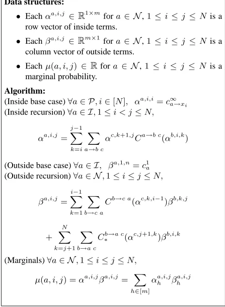
for alla∈ I. Data structures:

• Eachαa,i,j _{∈ R}1×m

fora ∈ N,1≤i≤j≤N is a row vector of inside terms.

• Eachβa,i,j

∈Rm×1 fora ∈ N,1≤i≤j≤N is a column vector of outside terms.

• Eachµ(a, i, j) ∈ Rfora ∈ N,1≤ i≤j ≤ Nis a marginal probability.

Algorithm:

(Inside base case)∀a∈ P, i∈[N], αa,i,i_=c∞

a→xi (Inside recursion)∀a∈ I,1≤i < j≤N,

αa,i,j =

j−1 X

k=i X

a→b c

αc,k+1,jCa→b c(αb,i,k)

(Outside base case)∀a∈ I, βa,1,n_=c1 a (Outside recursion)∀a∈ N,1≤i≤j≤N,

βa,i,j =

i−1 X

k=1 X

b→c a

Cb→c a(αc,k,i−1)βb,k,j

+

N X

k=j+1 X

b→a c

C∗b→a c(αc,j+1,k)β

b,i,k

(Marginals)∀a∈ N,1≤i≤j≤N, µ(a, i, j) =αa,i,jβa,i,j = X

h∈[m] αa,i,jh β

a,i,j h

Figure 3: The tensor form of the inside-outside algorithm, for calculation of marginal termsµ(a, i, j).

The outside tree contains everything in the s-tree

r1. . . rN, excluding the subtree below nodei. Our random variables are defined as follows. First, we select a random internal node, from a ran-dom tree, as follows:

• Sample an s-tree r1. . . rN from the PMF

p(r1. . . rN). Choose a nodeiuniformly at ran-dom from[N].

If the rulerifor the nodeiis of the forma→b c, we define random variables as follows:

•R1is equal to the ruleri(e.g.,NP→D N). •T1 is the inside tree rooted at node i. T2 is the inside tree rooted at the left child of nodei, andT3 is the inside tree rooted at the right child of nodei.

• A1, A2, A3 are the labels for node i, the left child of nodei, and the right child of nodei respec-tively. (E.g.,A1=NP,A2 =D,A3=N.)

•Ois the outside tree at nodei.

•Bis equal to1if nodeiis at the root of the tree (i.e.,i= 1),0otherwise.

If the rule ri for the selected node i is of

the form a → x, we have random

vari-ables R1, T1, H1, A1, O, B as defined above, but

H2, H3, T2, T3, A2, andA3are not defined.

We assume a functionψthat maps outside treeso

to feature vectorsψ(o)_∈Rd′. For example, the fea-ture vector might track the rule directly above the node in question, the word following the node in question, and so on. We also assume a function φ

that maps inside treestto feature vectorsφ(t)_∈Rd. As one example, the functionφmight be an indica-tor function tracking the rule production at the root of the inside tree. Later we give formal criteria for what makes good definitions ofψ(o) ofφ(t). One requirement is thatd′

≥mandd_≥m.

In tandem with these definitions, we assume pro-jection matices Ua _{∈ R}(d×m) _{and V}a _{∈ R}(d′_×m)

for alla ∈ N. We then define additional random variablesY1, Y2, Y3, Z as

Y1= (Ua1)⊤φ(T1) Z= (Va1)⊤ψ(O)

Y2= (Ua2)⊤φ(T2) Y3= (Ua3)⊤φ(T3)

where ai is the value of the random variable Ai. Note thatY1, Y2, Y3, Z are all inRm.

6.2 Observable Representations

Given the definitions in the previous section, our representation is based on the following matrix, ten-sor and vector quantities, defined for alla∈ N, for all rules of the forma→b c, and for all rules of the forma→xrespectively:

Σa = _E[Y1Z⊤|A1 =a]

Da→b c = E h

[[R1=a→b c]]Y3Z⊤Y2⊤|A1 =a i

d∞_a→x = E h

[[R1=a→x]]Z⊤|A1=a i

Assuming access to functionsφandψ, and projec-tion matricesUa_andVa_{, these quantities can be} es-timated directly from training data consisting of a set of s-trees (see section 7).

Our observable representation then consists of:

Ca→b c(y) = Da→b c(y)(Σa)−1 (2)

c∞_a→x = d

∞

a→x(Σa)

−₁

(3)

c1_a = _E[[[A1 =a]]Y1|B = 1] (4)

We next introduce conditions under which these quantities satisfy the conditions in theorem 1.

The following definition will be important:

Definition 2 For alla∈ N, we define the matrices

Ia_∈R(d×m)_andJa_∈R(d′_×m)

as

[Ia]i,h =E[φi(T1)|H1=h, A1=a]

[Ja]i,h=E[ψi(O)|H1 =h, A1 =a]

In addition, for any a _{∈ N}, we use γa _∈ Rm to denote the vector withγa

h=P(H1 =h|A1=a). The correctness of the representation will rely on the following conditions being satisfied (these are parallel to conditions 1 and 2 in Hsu et al. (2009)):

Condition 1 _∀a _{∈ N}, the matrices Ia _andJa_are

of full rank (i.e., they have rankm). For alla_{∈ N}, for allh_∈[m],γa

h>0.

Condition 2 ∀a ∈ N, the matrices Ua _{∈ R}(d×m)

andVa _∈R(d′_×m)

are such that the matricesGa₌

(Ua₎⊤

Ia_andKa_{= (V}a₎⊤

Ja_{are invertible.}

The following lemma justifies the use of an SVD calculation as one method for finding values forUa andVa_{that satisfy condition 2:}

Lemma 1 Assume that condition 1 holds, and for alla_{∈ N} define

Ωa=_E[φ(T1) (ψ(O))⊤|A1 =a] (5)

Then ifUa _{is a matrix of the m left singular}

vec-tors ofΩa _{corresponding to non-zero singular}

val-ues, andVa_{is a matrix of themright singular}

vec-tors ofΩa _{corresponding to non-zero singular}

val-ues, then condition 2 is satisfied.

Proof sketch: It can be shown that Ωa ₌

Ia_diag(γa_)(Ja₎⊤

. The remainder is similar to the proof of lemma 2 in Hsu et al. (2009).

The matricesΩacan be estimated directly from a training set consisting of s-trees, assuming that we have access to the functionsφandψ.

Theorem 2 Assume conditions 1 and 2 are satisfied. For alla_{∈ N}, defineGa _{= (U}a₎⊤

Ia_{. Then under}

the definitions in Eqs. 2-4:

1. For all rules a_→b c, Ca→b c_{(y) =}

Gc_Ta→b c_diag(yGb_Sa→b c_)Qa→b c_(Ga₎−₁

2. For all rulesa_→x,c∞

a→x= 1

⊤

Qa→x_(Ga₎−₁

.

3. For alla_{∈ N},c1_a=Ga_πa

Proof: The following identities hold (see

sec-tion 9.2):

Da→b c_{(y) =}

(6) GcTa→b cdiag(yGbSa→b c)Qa→b cdiag(γa)(Ka)⊤

d∞a→x= 1

⊤

Qa→xdiag(γa)(Ka)⊤ (7)

Σa_=Ga_diag(γa_)(Ka₎⊤

(8) c1a=G

a

πa (9)

Under conditions 1 and 2, Σa is invertible, and

(Σa₎−₁

= ((Ka₎⊤

)−1(diag(γa₎₎−₁

(Ga₎−₁

. The identities in the theorem follow immediately.

7 Deriving Empirical Estimates

Figure 4 shows an algorithm that derives esti-mates of the quantities in Eqs 2, 3, and 4. As input, the algorithm takes a sequence of tuples

(r(i,1)_{, t}(i,1)_{, t}(i,2)_{, t}(i,3)_{, o}(i)_{, b}(i)_)fori∈[M]. These tuples can be derived from a training set consisting of s-treesτ1. . . τM as follows:

• ∀i∈[M], choose a single nodejiuniformly at random from the nodes inτi. Definer(i,1) to be the rule at nodeji.t(i,1)is the inside tree rooted at node

ji. If r(i,1) is of the forma_→b c, thent(i,2) is the inside tree under the left child of nodeji, andt(i,3) is the inside tree under the right child of nodeji. If

r(i,1) _{is of the form a → x, then t}(i,2) _{= t}(i,3) ₌

NULL_{. o}(i) _{is the outside tree at nodeji. b}(i) _is1if

nodejiis at the root of the tree,0otherwise. Under this process, assuming that the s-trees

τ1. . . τM are i.i.d. draws from the distribution

p(τ) over s-trees under an L-PCFG, the tuples

(r(i,1)_{, t}(i,1)_{, t}(i,2)_{, t}(i,3)_{, o}(i)_{, b}(i)_{) are i.i.d. draws} from the joint distribution over the random variables

R1, T1, T2, T3, O, Bdefined in the previous section. The algorithm first computes estimates of the pro-jection matrices Ua _{and V}a_{: following lemma 1,} this is done by first deriving estimates of Ωa_, and then taking SVDs of each Ωa_{. The matrices} are then used to project inside and outside trees

t(i,1), t(i,2), t(i,3), o(i) down to m-dimensional vec-torsy(i,1), y(i,2), y(i,3), z(i); these vectors are used to derive the estimates ofCa→b c_,c∞

a→x, andc1a. We now state a PAC-style theorem for the learning algorithm. First, for a given L-PCFG, we need a couple of definitions:

•Λis the minimum absolute value of any element of the vectors/matrices/tensors c1_a, d∞

a→_x, Da→b c,

(Σa₎−1_{. (Note that Λ is a function of the} projec-tion matricesUa _{and V}a_{as well as the underlying} L-PCFG.)

• For each a _{∈ N}, σa _{is the value of the m’th} largest singular value ofΩa_{. Defineσ= min}

aσa. We then have the following theorem:

Theorem 3 Assume that the inputs to the algorithm in figure 4 are i.i.d. draws from the joint distribution over the random variablesR1, T1, T2, T3, O, B,

un-der an L-PCFG with distribution p(r1. . . rN) over

s-trees. Definem to be the number of latent states in the L-PCFG. Assume that the algorithm in fig-ure 4 has projection matricesUˆa_andVˆa_{derived as}

left and right singular vectors of Ωa_{, as defined in}

Eq. 5. Assume that the L-PCFG, together withUˆa

andVˆa_{, has coefficientsΛ>0andσ >0. In}

addi-tion, assume that all elements inc1 a,d

∞

a→x,Da

→b c_,

andΣa_{are in[−1,+1]. For any s-treer}

1. . . rN

de-fine pˆ(r1. . . rN) to be the value calculated by the

algorithm in figure 3 with inputs ˆc1_a, ˆc∞_a→_x,Cˆa →_{b c}

derived from the algorithm in figure 4. DefineRto be the total number of rules in the grammar of the forma_→b cora_→ x. DefineMato be the

num-ber of training examples in the input to the algorithm in figure 4 whereri,1_{has non-terminalaon its}

left-hand-side. Under these assumptions, if for alla

Ma≥

128m2

2N+1√_{1 +ǫ} −12

Λ2_σ4 log

2mR δ

Then

1₋ǫ_≤

ˆ

p(r1. . . rN)

p(r1. . . rN)

≤

1 +ǫ

A similar theorem (omitted for space) states that

1₋ǫ_≤ ˆ µ(a,i,j) µ(a,i,j)

≤1 +ǫfor the marginals.

The condition that Uˆa and Vˆa are derived from

applicable in deriving results for the case whereΩˆa is used in place ofΩa_.

Proof sketch: The proof is similar to that of Foster

et al. (2012). The basic idea is to first show that under the assumptions of the theorem, the estimates

ˆ

c1_a,dˆ∞_a→_x,Dˆa →_{b c}

,Σˆa_{are all close to the underlying} values being estimated. The second step is to show that this ensures thatp(rˆ 1...rN′)

p(r1...rN′)is close to1.

The method described of selecting a single tuple

(r(i,1), t(i,1), t(i,2), t(i,3), o(i), b(i))for each s-tree en-sures that the samples are i.i.d., and simplifies the analysis underlying theorem 3. In practice, an im-plementation should most likely use all nodes in all trees in training data; by Rao-Blackwellization we know such an algorithm would be better than the one presented, but the analysis of how much better would be challenging. It would almost certainly lead to a faster rate of convergence ofpˆtop.

8 Discussion

There are several potential applications of the method. The most obvious is parsing with L-PCFGs.1The approach should be applicable in other cases where EM has traditionally been used, for ex-ample in semi-supervised learning. Latent-variable HMMs for sequence labeling can be derived as spe-cial case of our approach, by converting tagged se-quences to right-branching skeletal trees.

The sample complexity of the method depends on the minimum singular values ofΩa_{; these singular} values are a measure of how well correlated ψand

φare with the unobserved hidden variableH1. Ex-perimental work is required to find a good choice of values forψandφfor parsing.

9 Proofs

This section gives proofs of theorems 1 and 2. Due to space limitations we cannot give full proofs; in-stead we provide proofs of some key lemmas. A long version of this paper will give the full proofs.

9.1 Proof of Theorem 1

First, the following lemma leads directly to the cor-rectness of the algorithm in figure 2:

1

Parameters can be estimated using the algorithm in figure 4; for a test sentence x1. . . xN we can first use the algorithm in figure 3 to calculate marginals µ(a, i, j), then use the algorithm of Goodman (1996) to find

arg maxτ∈T(x)P(a,i,j)∈τµ(a, i, j).

Inputs: Training examples(r(i,1)_{, t}(i,1)_{, t}(i,2)_{, t}(i,3)_{, o}(i)_{, b}(i)₎ fori ∈ {1. . . M}, wherer(i,1)_{is a context free rule; t}(i,1)_, t(i,2) and t(i,3) are inside trees; o(i) is an outside tree; and b(i)= 1if the rule is at the root of tree,0otherwise. A function φthat maps inside treestto feature-vectorsφ(t)∈Rd. A func-tionψthat maps outside treesoto feature-vectorsψ(o)∈Rd′. Algorithm:

Defineaito be the non-terminal on the left-hand side of rule r(i,1)_{. Ifr}(i,1)_{is of the forma→b c, definebito be the} non-terminal for the left-child ofr(i,1)_{, andcito be the non-terminal} for the right-child.

(Step 0: Singular Value Decompositions)

• Use the algorithm in figure 5 to calculate matricesUˆa_∈ R(d×m)andVˆa

∈R(d′×m)for eacha∈ N. (Step 1: Projection)

• For alli∈[M], computey(i,1)= ( ˆUai₎⊤_φ(t(i,1)_). • For all i ∈ [M] such that r(i,1) is of the form

a→b c, computey(i,2)_{= ( ˆU}bi₎⊤_φ(t(i,2)_)andy(i,3)₌

( ˆUci₎⊤_φ(t(i,3)_).

• For alli∈[M], computez(i)_{= ( ˆV}ai₎⊤_ψ(o(i)_). (Step 2: Calculate Correlations)

• For eacha∈ N, defineδa= 1/PM_i=1[[ai=a]]

• For each rule a→b c, compute Dˆa→b c _{= δa} × PM

i=1[[r

(i,1)_{=a→b c]]y}(i,3)_(z(i)₎⊤

(y(i,2)₎⊤

• For each rule a → x, compute dˆ∞

a→x = δa × PM

i=1[[r

(i,1)_=a→x]](z(i)₎⊤

• For each a ∈ N, compute Σˆa _{= δa ×} PM

i=1[[ai=a]]y(i,1)(z(i))

⊤

(Step 3: Compute Final Parameters)

• For alla→b c,Cˆa→b c_{(y) = ˆD}a→b c_{(y)( ˆΣ}a₎−1 • For alla→x,cˆ∞

a→x= ˆd

∞

a→x( ˆΣa)

−1

• For alla∈ I,cˆ1a=

PM

i=1[[a_Pi=aandb(i)=1]]y(i,1) M

i=1[[b(i)=1]]

Figure 4: The spectral learning algorithm.

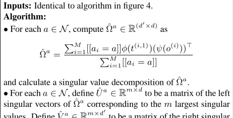
Inputs: Identical to algorithm in figure 4. Algorithm:

•For eacha∈ N, computeΩˆa_∈R(d′×d) as

ˆ Ωa₌

PM

i=1[[ai=a]]φ(t(i,1))(ψ(o(i)))

⊤

PM

i=1[[ai=a]]

and calculate a singular value decomposition ofΩˆa . •For eacha∈ N, defineUˆa_∈

Rm×dto be a matrix of the left singular vectors ofΩˆa

corresponding to themlargest singular values. DefineVˆa_∈Rm×d′

to be a matrix of the right singular vectors ofΩˆa

corresponding to themlargest singular values.

Lemma 2 Assume that conditions 1-3 of theorem 1 are satisfied, and that the input to the algorithm in figure 2 is an s-treer1. . . rN. Defineai fori∈[N]

to be the non-terminal on the left-hand-side of rule

ri, and ti for i ∈ [N] to be the s-tree with rule ri

at its root. Finally, for alli ∈ [N], define the row vectorbi_∈R(1×m)_{to have components}

bi_h=P(Ti=ti|Hi =h, Ai =ai)

forh_∈[m]. Then for alli_∈[N],fi_=bi_(G(ai)₎−1_.

It follows immediately that

f1c1_a1 =b1(G(a1)₎−1_Ga1_π

a1 =p(r1. . . rN)

This lemma shows a direct link between the vec-torsfi_{calculated in the algorithm, and the termsb}i

h, which are terms calculated by the conventional in-side algorithm: each fi _{is a linear transformation} (throughGai_{) of the corresponding vectorb}i_.

Proof: The proof is by induction.

First consider the base case. For any leaf—i.e., for anyisuch thatai ∈ P—we havebih = q(ri|h, ai), and it is easily verified thatfi_=bi_(G(ai)₎−1_.

The inductive case is as follows. For alli ∈ [N]

such thatai ∈ I, by the definition in the algorithm,

fi = fγCri_(fβ₎

= fγGaγ_Tri_diag(fβ_Gaβ_Sri_)Qri_(Gai₎−1

Assuming by induction thatfγ _=bγ_(G(aγ)₎−1 _and

fβ _=bβ_(G(aβ)₎−1_{, this simplifies to}

fi =κrdiag(κl)Qri_(Gai₎−1 ₍₁₀₎

where κr _{= b}γ_Tri_{, andκ}l _{= b}β_Sri_{. κ}r _{is a row}

vector with componentsκr h =

P h′_∈[m]b

γ

h′T_hr′i_,h =

P

h′_∈[m]bγ_h′t(h

′

|h, ri). Similarly,κlis a row vector with components equal toκl

h= P

h′_∈[m]bβ_h′S

ri

h′_,h=

P h′_∈[m]b

β h′s(h

′

|h, ri). It can then be verified that

κr_diag(κl_)Qri _{is a row vector with components}

equal toκr

hκlhq(ri|h, ai). Butbi

h =q(ri|h, ai)×

P

h′_∈[m]bγ_h′t(h

′

|h, ri)

×

P

h′_∈[m]bβ_h′s(h

′

|h, ri)

= q(ri|h, ai)κrhκlh, hence

κrdiag(κl)Qri _{= b}i _{and the inductive case follows}

immediately from Eq. 10.

Next, we give a similar lemma, which implies the correctness of the algorithm in figure 3:

Lemma 3 Assume that conditions 1-3 of theorem 1 are satisfied, and that the input to the algorithm in figure 3 is a sentencex1. . . xN. For anya∈ N, for

any1_≤i_≤j _≤N, defineα¯a,i,j _∈R(1×_m)

to have componentsα¯a,i,j_h =p(xi. . . xj|h, a)forh ∈ [m].

In addition, defineβ¯a,i,j _{∈ R}(m×₁₎

to have compo-nentsβ¯_ha,i,j = p(x1. . . xi−₁, a(h), x_j+1. . . xN) for

h∈[m]. Then for alli∈[N],αa,i,j _{= ¯α}a,i,j_(Ga₎−1

andβa,i,j _=Ga_β¯a,i,j_{. It follows that for all(a, i, j),}

µ(a, i, j) = ¯αa,i,j(Ga)−1Gaβ¯a,i,j = ¯αa,i,jβ¯a,i,j

=X

h

¯

αa,i,j_h β¯_ha,i,j = X

τ∈T(x):(a,i,j)∈τ

p(τ)

Thus the vectorsαa,i,j _{and β}a,i,j _{are linearly} re-lated to the vectorsα¯a,i,j _{and β¯}a,i,j_{, which are the} inside and outside terms calculated by the conven-tional form of the inside-outside algorithm.

The proof is by induction, and is similar to the proof of lemma 2; for reasons of space it is omitted.

9.2 Proof of the Identity in Eq. 6

We now prove the identity in Eq. 6, used in the proof of theorem 2. For reasons of space, we do not give the proofs of identities 7-9: the proofs are similar.

The following identities can be verified:

P(R1=a→b c|H1=h, A1 =a) = q(a→b c|h, a) E[Y3,j|H1=h, R1 =a→b c] = Ej,ha→b c

E[Zk|H1=h, R1 =a→b c] = Kk,ha E[Y2,l|H1=h, R1 =a→b c] = Fl,ha→b c

whereEa→b c _=Gc_Ta→b c_,Fa→b c _=Gb_Sa→b c_.

Y3, Z andY2 are independent when conditioned onH1, R1 (this follows from the independence as-sumptions in the L-PCFG), hence

E[[[R1=a→b c]]Y3,jZkY2,l|H1=h, A1=a]

= q(a_→b c_|h, a)E_j,ha→b cK_k,ha F_l,ha→b c

Hence (recall thatγa

h =P(H1=h|A1 =a)),

D_j,k,la→b c=_E[[[R1 =a→b c]]Y3,jZkY2,l |A1 =a]

= X

h

γ_haE[[[R1 =a→b c]]Y3,jZkY2,l |H1 =h, A1 =a]

= X

h

γ_haq(a_→b c_|h, a)E_j,ha→b cK_k,ha F_l,ha→b c (11)

Acknowledgements: Columbia University gratefully ac-knowledges the support of the Defense Advanced Re-search Projects Agency (DARPA) Machine Reading Pro-gram under Air Force Research Laboratory (AFRL) prime contract no. FA8750-09-C-0181. Any opinions, findings, and conclusions or recommendations expressed in this material are those of the author(s) and do not nec-essarily reflect the view of DARPA, AFRL, or the US government. Shay Cohen was supported by the National Science Foundation under Grant #1136996 to the Com-puting Research Association for the CIFellows Project. Dean Foster was supported by National Science Founda-tion grant 1106743.

References

B. Balle, A. Quattoni, and X. Carreras. 2011. A spec-tral learning algorithm for finite state transducers. In

Proceedings of ECML.

S. Dasgupta. 1999. Learning mixtures of Gaussians. In

Proceedings of FOCS.

Dean P. Foster, Jordan Rodu, and Lyle H. Ungar. 2012. Spectral dimensionality reduction for hmms. arXiv:1203.6130v1.

J. Goodman. 1996. Parsing algorithms and metrics. In

Proceedings of the 34th annual meeting on Associ-ation for ComputAssoci-ational Linguistics, pages 177–183.

Association for Computational Linguistics.

D. Hsu, S. M. Kakade, and T. Zhang. 2009. A spec-tral algorithm for learning hidden Markov models. In

Proceedings of COLT.

H. Jaeger. 2000. Observable operator models for discrete stochastic time series. Neural Computation, 12(6). F. M. Lugue, A. Quattoni, B. Balle, and X. Carreras.

2012. Spectral learning for non-deterministic depen-dency parsing. In Proceedings of EACL.

T. Matsuzaki, Y. Miyao, and J. Tsujii. 2005. Proba-bilistic CFG with latent annotations. In Proceedings

of the 43rd Annual Meeting on Association for Com-putational Linguistics, pages 75–82. Association for

Computational Linguistics.

A. Parikh, L. Song, and E. P. Xing. 2011. A spectral al-gorithm for latent tree graphical models. In

Proceed-ings of The 28th International Conference on Machine Learningy (ICML 2011).

F. Pereira and Y. Schabes. 1992. Inside-outside reesti-mation from partially bracketed corpora. In

Proceed-ings of the 30th Annual Meeting of the Association for Computational Linguistics, pages 128–135, Newark,

Delaware, USA, June. Association for Computational Linguistics.

S. Petrov, L. Barrett, R. Thibaux, and D. Klein. 2006. Learning accurate, compact, and interpretable tree an-notation. In Proceedings of the 21st International

Conference on Computational Linguistics and 44th Annual Meeting of the Association for Computational Linguistics, pages 433–440, Sydney, Australia, July.

Association for Computational Linguistics.

S. A. Terwijn. 2002. On the learnability of hidden markov models. In Grammatical Inference:

Algo-rithms and Applications (Amsterdam, 2002), volume

2484 of Lecture Notes in Artificial Intelligence, pages 261–268, Berlin. Springer.

S. Vempala and G. Wang. 2004. A spectral algorithm for learning mixtures of distributions. Journal of