Munich Personal RePEc Archive
Revisiting the causal effects of exporting
on productivity: Does price
heterogeneity matter?
Wassie, Tewodros Ayenew
Department of Economics, University of Sheffield
1 July 2017
Online at
https://mpra.ub.uni-muenchen.de/80576/
Revisiting the causal effects of exporting on productivity: Does price
heterogeneity matter?
Tewodros Ayenew Wassie
Department of Economics, University of Sheffield, UK
Abstract
This paper examines the causal effect of exporting on firms’ productivity controlling for price heterogeneity. In most empirical studies that establish the export-productivity relationships, output is measured in values rather than in quantities. This makes it difficult to distinguish between productivity and within-firm changes in price that may occur following exposure to international markets. Using a detail data on quantity and prices from Ethiopian manufacturing firms in the period 1996-2005, this paper distinguishes efficiency from revenue based productivity and examines what this means for the estimated relationship between exporting and productivity. The empirical strategy implemented in the paper allows for potential endogeneity for exporting and controls for self-selection into export. The main results show that exporters are more productive than non-exporters in terms of revenue based productivity and this is explained by both self-selection and learning effects. However, when correcting for price heterogeneity using quantity-based measures of productivity, exporters appear to be similar to non-exporters either before or after export entry. Overall, the results suggest that the observed relationship between exporting and productivity mainly occurs through price mechanism.
Keywords: Export; revenue productivity; physical productivity; price heterogeneity; fixed effect
quantile regression
JEL codes: F14, D22, O55
The obligatory copyright note: I certify that I have the right to deposit the contribution with
MPRA.
1 Introduction
The fact that recent studies find a systematic difference between exporters and non-exporters in terms of price (reflecting quality) (Kugler and Verhoogen, 2012; Iacovone and Javorcik, 2012) makes identifying the actual relationship between exporting and productivity more complicated. That is, part of the productivity differential may result from the price premium of exporters. In a related study Gervais (2015) finds that product quality is more important than physical productivity in determining frims selection into foreign markets. Most pointedlyDe Loecker(2011) cautions inferring the productivity effects using deflated revenue as an output measure showing that correcting price heterogeneity leads to a substantially reduced productivity gains associated with trade liberalization. This study specifically begs for serious revisions of the earlier results in the literature by addressing the role of demand side factors. However, there is a dearth of evidence when it comes to how would taking into account price (and thus demand) differences across firms would shape the relationship between export and productivity. A notable exceptions in this regard isSmeets and Warzynski(2013) that examines the link between trade and productivity taking into account price heterogeneity for Danish manufacturing firms.
This paper therefore re-examines the causal effects of exporting on productivity accounting for price heterogeneity. It differs from previous studies as it does not focus on the the relationship between exporting and productivity per se but the the impact of price heterogeneity in the estimated link between exporting and productivity. To this end, I exploit the richness of quantity and price information from a large panel of Ethiopian manufacturing firms in the period 1996-2005 and estimate two conceptually distinct productivity measures introduced by (Foster et al., 2008). The first one is revenue productivity (TFPR) which is estimated from revenue production function. This is essentially the standard TFP measures that is widely used in earlier empirical studies. The second is physical productivity (TFPQ) estimated using firm-level quantity (price) information and thus not affected by price differences across firms.
In identifying the impact of exporting on productivity, the empirical strategy of this paper controls for unobserved firm heterogeneity along with two well-known sources of bias: potential endogeneity of export activities in firms production decision and self-selection into export. This is carried out by estimating export augmented dynamic production function applying system Gen-eralised Method of Moments (GMM) estimator while simultaneously controlling for self-selection using Propensity Score Matching (PSM) technique. Departing from average relationship, the pa-per further investigates the productivity gap between exporters and non-exporters over the whole productivity distribution. In doing so, it implements fixed effect quantile estimator that accounts for unobserved firm heterogeneity. To asses how price heterogeneity may affect the measured pro-ductivity and the estimated relationship between exporting on propro-ductivity, the results obtained when using revenue (or revenue-based productivity) are compared to those obtained using quantity (or quantity-based productivity)
domestic and foreign markets.1 The alternative learning-by-exporting view predicts that exporting
increases productivity due to knowledge flows from foreign buyers and the pro-competitive effect of participating in international markets (Clerides et al.,1998;Aw et al.,2000).
While empirical evidence on self-selection dominates in studies from developed countries, learn-ing effect is largely documented in developlearn-ing countries (ISGEP, 2008;Wagner, 2007, 2012). On the other hand, studies for Sub-Saharan Africa (SSA) firms show the complementarity of the two effects (Bigsten et al.,2004;Van Biesebroeck,2005). Individual country studies provide consistent results. Bigsten and Gebreeyesus(2009) find the presence of both selection and learning effects of exporting for firms in Ethiopia. A most recent study however shows that the pre-export productiv-ity advantage of Ethiopian exporters is mainly driven by firm fixed effects (Siba and Gebreeyesus, 2017). In general, based on a meta analysis of empirical papers including firm-level studies from SSA, Martins and Yang (2009) conclude that the effect of exporting on productivity is larger for firms in developing countries.
This paper makes several important contributions to the literature on firm heterogeneity and trade. First of all, it explains the observed export variations by two distinctive margins that are confounded in revenue productivity: physical productivity and prices. This sheds some light on the source of the productivity difference between exporters and non-exporters that have been found in previous studies particularly focusing on African firms. Secondly, it confirms the importance of both self-selection and learning effects in explanting the superior revenue productivity of exporters in developing countries. Despite the evidence on the complementarity of selection and learning effects for firms in Africa, to the best of my knowledge this is the first paper that takes into account the impact of price heterogeneity. Thus, the results should offer some important insights into the possible biases that may occur in the absence of detail price data, especially for future studies focusing on firms in other developing countries.
Moreover, this analysis is particularly relevant for less industrialised countries which strive to build manufacturing-based sustainable economy. In this regard, Ethiopia represents an interesting case to study. Typical to many SSA countries, the Ethiopian manufacturing sector is dominated by small-sized firms with poor export performance where less than 5% of firms export. On the other hand, the country is one of the few African economies that have been implementing successive in-dustrial policy reforms aiming at developing export-oriented labor-intensive manufacturing sector. Specifically, since the early 2000s the government has identified strategic export sectors and set quantitative productivity targets as a means to improve the export performance of the manufac-turing industry2. Despite this effort, the performance of the sector remains poor raising concerns on the effectiveness of industrial promotion policies that solely focus on increasing quantity output. Furthermore, unlike many countries in the region, the country conducts a census of manufacturing firms annually collecting detail plants/product-level information including value and quantity of productions. The Ethiopian context provides a unique opportunity to disentangle the various firm-specific characteristics embodied in the empirically estimated revenue based productivity in the SSA context and examine their separate impact on export performance. Therefore, providing the first evidence on the relative importance of demand and supply side factors in determining firms selection into export, this paper could contribute to the policy debate aiming to foster international
1
Challenging the exogenous productivity assumption, Lopez (2004) introduces the concept of conscious self-selection: selection into export is a result of conscious investment decisions by forward-looking firms that aim to improve their productivity with explicit purpose of becoming exporters. Empirical studies, especially from develop-ing countries, find supportdevelop-ing evidence on the conscious self-selection hypothesis (for example see (Espanol,2007)).
2
competitiveness of firms in the region.
The results confirm the earlier evidence in the literature that higher revenue based productiv-ity is associated with exporting in both pre- and post-export entry. However, correcting for price heterogeneity in estimating productivity leads to insignificant causal effects of exporting on pro-ductivity. The results show that the now standard approach of examining the relationship between exporting and productivity using revenue based productivity measure masks important source of heterogeneity. Specifically, the paper highlights the potential bias of ignoring price heterogeneity as the price premium of exporting firms could simply be translate into higher revenue productivity. The remainder of this paper is organised as follows. Section2outlines the conceptual framework of the paper focusing on the implications of price heterogeneity in estimating productivity. Section 3 presents the empirical models and estimation strategies. Section 4 provides the description of the data along with some facts that help interpret the empirical results. Section 5 presents the empirical results and section6 concludes.
2 Conceptual Framework
This section shows how ignoring price differences across firms affects productivity estimates and its implication on the estimated relationship between export and productivity. Thus, let us start with a logarithmic representation of a Cobb-Douglas production function that relates output with inputs as follow
qit =
X
x
βxxit+ωit+ǫit; (1)
where qit is quantity output of firm i in period t; x =
n
l, m, ko are quantity of labor, intermedi-ate inputs and capital, respectively ; ωit measures total factor productivity (TFP), all in natural
logarithms; ǫit represents firm- and time-specific deviations from mean productivity. With
fur-ther assumption that ǫit can be decomposed into predictable and unpredictable components, the
logarithm of firm-level TFP is empirically estimated as a residual from the production function estimates.
Essentially, productivity measures output differences that cannot be explained by input differ-ences. Thus, obtaining an accurate productivity estimate requires output and input quantities, which are not typically available in many firm-level data-sets. The standard practice by researchers is therefore deflating firm-level sales and input expenditures by industry-level price indices and then use the deflated values of inputs and outputs as a proxy for their quantities. Thus, the production function actually estimated in empirical studies is the following
˜ rit=
X
x
βx(x˜it+pxit−p¯ktx) + (pit−p¯kt) +ωit+ǫit (2)
where ˜rit is firm-level deflated revenue; ˜xit is deflated input expenditures;pit is the output price of
firm i; ¯pkt is the average price of industry k that the firm belongs to; pxit is firm specific price of
inputx; ¯px
kt is average industry-level price of inputx, all in logarithms. It is clear that in addition
to the real productivity measure (ωit) and the error term, this revenue production function contains
output price error (pit−p¯kt) and input price errors (pxit−p¯xkt) capturing the deviations of
In the presence of imperfect competition where there is within industry price heterogeneity, the use of deflated values as a substitute for quantities raises two important concerns. First, if choice of inputs is correlated with the unobserved firm price differences, the estimated input coefficients would be biased (Klette et al.,1996;Levinsohn and Melitz,2002). Second, it leads to a significant bias in the estimated productivity favouring firms that charge higher prices. Specifically, (Foster et al., 2008) note that if a firm charges a price level above the average industry price, the use deflated revenue as a proxy for quantity output results in higher output for a given input. This in turn overstates the productivity of high price firms. A related possibility is that the productivity measure estimated from revenue production functions captures the difference between revenue and expenditures thus it is closely related to profitability that depends not only on physical efficiency but also on price (De Loecker and Goldberg,2014).
Foster et al. (2008) examine the difference between TFP estimates obtained when using firm sales deflated by industry price, called revenue productivity (TFPR) to those obtained when using firm sales deflated by firm-level price, called physical productivity (TFPQ) and their impact of firms selection into markets. Their findings suggest that the revenue productivity of young firms entering into a market is underestimated simply because on average they charge lower prices than incumbent firms. Similarly,Siba and S¨oderbom(2011) find a supporting evidence for Ethiopian manufacturing firms in which new market entering firms have lower demand and price than established firms, but they do not significantly differ in terms of physical productivity.
The evidence from these studies suggests that comparing the revenue productivity of firms that have different pricing strategies would be misleading. This is because despite efficiency similarities, lower average revenue productivity for a group of firms could be due to their relative lower output prices. Given the recent evidence that exporters on average charge higher prices than non-exporters such as byKugler and Verhoogen(2012) andIacovone and Javorcik(2012), this argument underpins the importance of re-examining the impact of ignoring price heterogeneity in the estimated link between exporting and productivity. Specifically, higher average price for exporters implies that the tradition of using revenue deflated by a common deflator as a measure of output in estimating productivity would result in a disproportionately higher revenue productivity for exporters.
3 Empirical Strategy
The main objective of this paper is to investigate whether there is evidence on self-selection into exporting and learning by exporting focusing on how taking into account price heterogeneity affects the estimated relationship between exporting and productivity. Therefore, the main focus is obtaining productivity measure not affected by price bias. Since price bias arises when productivity is estimated using firm revenue deflated by common industry-level price, it can be controlled using quantity information. To address this issue followingFoster et al. (2008) this paper uses quantity (firm-level price) data to estimate quantity based productivity (TFPQ) which is not affected by price variations. To compare with earlier studies, the traditional revenue based productivity (TFPR) is also estimated using firm sale deflated by industry price indices. Then, the impact of price heterogeneity in the estimated relationship between exporting and productivity is examined by comparing results obtained when using TFPR with those obtained when using TFPQ. This is similar to the approach used by Smeets and Warzynski(2013).
3.1 Export premium and productivity heterogeneity
each firm in the sample. I use firm-level data to estimate the production function specified in equation (1) for each each 2-digit industry separately. The estimated parameters are then used to derive firm-specific TFP. To overcome the well known bias due to simultaneity between productivity socks and input choices, I apply the system Generalised Method of Moments (GMM) estimator of Blundell and Bond(1998). Once collecting the TFP measures, the following standard specification is estimated to compute export premium:
TFPit=β0+βexExpit+βlEmplit+ψi+sit+γt+εit (3)
whereT F Pit is TFPR or TFPQ in alternative specifications,Expit is a dummy which equals 1 if a
firm exports at time t and zero otherwise and βex measures the percentage productivity premium
of exporters. The model also controls for log of employment(Emplit) as a proxy for firm size; ψi,
sit and γt are firm, industry and time fixed effects, respectively. To better interpret the source
of export premium, I run the following model that distinguish the relative importance of always exporters, switchers and starters:
TFPit=β0+φExpalwi +δExpstarti +σExpiswitch+βlEmplit+sit+γt+εit (4)
where Expalwi is a dummy for always exporters, Expstarti is dummy for export starters, Expswitchi is a dummy for export switchers. Other variables are defined as before. The base line group is firm that never export in all the years. Thus, the coefficients of the different types of export status captures the percentage difference between that particular type of exporter and never exporters.
The export premium estimated in the above way compares an average exporter with an average non-exporter with an implicit assumption that the export premium is evenly distributed across the productivity distribution. However, given that firm heterogeneity is the very fabric of this literature, there is no reason to believe average relationship reveals the full story. The Ethiopian data also shows that exporters themselves are highly heterogeneous and there are low productive exporters and high productive non-exporters. Furthermore, some firms are far from the mean productivity of the sample (see section 4.2). Thus, the analysis based on the average relationships may miss crucial questions whether exporting is correlated with productivity differently at a different level of productivity and whether the export-productivity correlations are driven by outliers. To address this issue, the paper estimates the relationships between exporting and productivity on the full productivity distributions using quantile regression.
In addition to cross-sectional quantile analysis, I account for the potential bias due to unob-served firm heterogeneity applying fixed-effect quantile estimator developed byCanay (2011). The application of this estimator starts with transforming the data such that the firm-specific fixed effects are eliminated. Consider a function that relates TFP with exporting activities and other controls:
T F Pit=X
′
itβ+αi+εit (5)
where E(εit|Xit, αi) = 0; Xit captures the set of time-varying variables including export status;
αi is firm fixed-effect; andεit is the standard error term. The firm-fixed effect is defined as ˆαi ≡
E[T F Pit−X
′
itβˆ]; where E[.] = T−1 T
P
t=1
[.]; and ˆβ is the within estimator of β. The fixed effect is
removed from the TFP as ˆT F Pit=T F Pit−αiˆ . Then, the standard quantile regression estimator
3.2 Selection into export
The presence of self-selection into export is tested by comparing the pre-export entry produc-tivity of exporters and non-exporters (Bernard and Jensen, 1999; ISGEP,2008). The idea is that if higher productive firms self-select into foreign markets, future exporters should show higher pro-ductivity than non-exporters several years before some of them begin to export. This is carried out by regressing productivity dated at τ on export status at export entry period tas follows:
T F Pi,t−τ =β0+βexp0Expit0+βlEmplit−τ+sit−τ+γt+εit (6)
whereT F P is eitherT F P R orT F P Q, Expit0 is export status at the export entry period (t= 0) and equals to one for export starters and zero for never-exporters, Emp is firm employment; sit
and γt are industry and time fixed effects, respectively; t is the year of entry into foreign market
for export starters and the median year for non-exporters. The sample used to estimate this model contains export starters and never exporters only. The interest lies on βexp0 in which a positive and significant coefficient implies that a firm that enters into export market at timet outperform never exporters at t−s years back when all of them did not export. However, it is important to emphasise that the results do not establish causal relationships. The pre-export performance difference is assessed from one (τ = 1) to three (τ = 3) years back prior to entry.
3.3 Effects of exporting
There are two main identification issues in estimating the effect of exporting on productivity. First, firms may make export decision input choices simultaneously which could lead to biased estimates. To overcome this, I augment export status in the production function so that the parameters of the production function and the effect of export are estimated simultaneously. This approach enables to control for the presence of unobserved correlation between exporting and productivity and thus identify the effects of exporting. The model also allows for persistence in firm-level productivity such that it follows a first-order autoregressive process yielding the following dynamic representation of the production function estimated in this paper:
qit=αqit−1+
X
x
βxxit+βexExpit−1+sit+γt+ψi+εit (7)
whereqitandqit−1 are the log of output of the firm in periodtandt−1;Expit−1 is a dummy for the firm previous year export status;P
x
βx= (βl, βm, βk) are the coefficients ofl,mandk, respectively;
Expit−1 is previous period export status; ψi represents unobserved firm-specific effect; sit and γt
capture industry-specific and year-specific intercepts respectively; εit is an iid error term ǫit is
serially uncorrelated measurement error. The underpinning principle for this specification is that firms are heterogeneous in their underlying productivity; and if firms learn from foreign markets, their previous export participation should determine their current productivity. Therefore, the parameter of interest is βex where a positive and significant coefficient indicates the presence of
learning effect from exporting.
differences as instrument for equations in levels and lags of variables in levels as instrument for the first-differenced equations. All inputs and export variables are taken as endogenous while industry and year indicators are treated as exogenous. The model is estimated by two-step GMM estimation allowing forWindmeijer(2005) correction, which adjusts the covariance matrix for finite sample to minimise the downward bias in standard errors.
The GMM estimator has been widely employed in recent empirical work, particularly stud-ies on productivity and firm export behaviour, particularly in the African context (Bigsten and Gebreeyesus,2009;Van Biesebroeck,2005). This method has a number of advantages. GMM esti-mator could provide consistent parameter estimates when the regressors are potentially endogenous and allow for persistency of productivity and firm heterogeneity. Further, using simulated sample of firms, Van Biesebroeck (2007) shows that system GMM provides the most robust estimates in the presence of measurement errors and technological heterogeneity, which are typical to many developing countries scenarios.
The other issue is selection bias that occurs as exporting firms may posses certain character-istics such that they would achieve better performance than non-exporters even if they did not export. Specifically, as more productive firms are more likely to export, it is impossible to differen-tiate whether the post-export productivity difference between exporters and non-exporters is due to their participation into foreign markets or difference between them in terms of other pre-export characteristics. Ideally, dealing with the selection bias requires obtaining counterfactual outcome (productivity) that exporters would realise on average in the absence of export participation. As in Girma et al. (2004), the unobserved counterfactual productivity of exporters is obtained im-plementing Propensity Score Matching (PSM) technique in which every exporting firm is paired with another non-exporting firm with similar observable characteristics. This exercise is carried out first by constructing a matched sample of exporters and non-exporters based on propensity score estimated from the following export decision equation:
P(Expit = 1) =f(lnLit−1, ln(K/L)it−1, lnAgeit−1, P ublic, Indu, year) (8)
whereExpit captures the export status of the firm; Lcaptures firm size; (K/L) represents capital
intensity; Age is the age of the firm; P ublic is dummy for public paid up capital contributions; Indu and year represent a full set of dummies for industry and years, respectively. The closest match for each exporting firm is established using nearest-neighbourhood approach based on the probability of exporting (propensity score).3 Then, the learning effect is examined using only the matched sample.
Keeping in mind that the main interest of this paper is to disentangle the within-firm physical efficiency gains from changes in price as a result of export, two alternative output measures are used: deflated revenue and quantity output. The idea behind this exercise is that since deflated revenue embody both efficiency and price differences, a positive export effect on it could partly be due to its effect on price. Thus, the use physical output which is not contaminated by firm-level price variations enables us to identify the pure effect of export on firm’s efficiency.
3
The estimation is carried out using TFPR and TFPQ as an outcome variables in Stata psmatch2 package (see
4 Data and Descriptive Evidence
4.1 Data source and summary statistics
The data used for the analysis come from the annual Ethiopian Large and Medium Scale Manufacturing Enterprise Census run by the Central Statistical Agency of Ethiopia (CSA). The manufacturing census covers all major manufacturing sectors in all regions of the country based on 4-digits international standard industrial classification (ISIC). The data used here covers periods from 1996 to 2005, at annual interval. The unit of observation in the sample is plant and all plant with 10 or more employees that use power-driven machinery are covered in the survey4. All plants
are uniquely identified and the data contain fairly detail information including total sales value, value of export, number of permanent and temporary employees, book value of fixed assets at the beginning and the end of the year, investment on fixed assets, current and initial paid up capital from domestic (private and public) and foreign sources, value of imported and local raw materials, costs of energy and other inputs, year of establishment, ISIC codes and geographical location of the plant.
The unique feature of the data is that it contains plant-product level information on value and quantity of sales in domestic and foreign markets. Plants report up to 9 product lists and CSA provides certain codes for these products which are defined consistently across sector and years. For example, the list of products in beverage sector (3-digit ISIC 155 ) are liquor, wine, beer, malt, lemonade (soft drinks) and mineral water. The data also provides standard unit of measurement such as litre, kilogram, pieces and square meter for each product depending on the sector. After standardising product-level quantity output in comparable measurement units, I compute firm-level quantity and price used to estimate quantity based productivity. Analogous to output information, the data provides information-though incomplete- for the value and quantity of raw materials used by firms. This information is used to construct firm-level raw material price used in the robustness check of this paper. The data is also used to construct other variables of interest such as exporting activities, employment, capital, investment and ownership. The details on the construction of the variables and data cleaning are presented in Appendix A.1.
Using the export information, first firms are grouped into two groups: exporters, firms that report positive export value in the current period and non-exporters those firms with zero export value in the current period. This classification enables to evaluate the average difference between exporters and non-exporters. To differentiate different types of exporters and identify their rela-tionship with productivity, firms are further classified into four groups: (i) Never exporters are firms that report zero export values all the time in the sample period; (ii) Always exporters are firms that report positive export sales in all years throughout the sample period; (iii) New exporters are firms that start to export at some point in the sample period and continues to export through the end; (iv) Export switchers are those firms that change their export status more than once.
Table 1 presents the size (output and employment) of all firms in the sample period. The number of firms covered in the census increased over time from 623 in 1996 to 997 in 20045. On the other hand, the average number of employees decreases over time. One possible reason for
4
Though the unit of observation in the data is plant, most Ethiopian manufacturing firms have a single plant and the distinction between firm and establishment is somehow blurred. Thus, firm and plant will be used interchangeably throughout the paper.
5
this declining trend of average employment can be that small firms that marginally passed the 10 employment threshold required to be included in the survey have joined the recent years’ surveys. In fact, the large gap between the median (137) and the mean (28) indicates a high skewness of the size distribution towards left reflecting the dominance of small firms in the manufacturing sector. The mean of the manufacturing output mostly increases over time, though its distribution skewed towards the left.
Table 1: Output and Employment over time
Employment Output
Year No. Firms Mean Median Mean Median
1996 623 149.77 22.67 880.90 55.10
1997 697 139.03 23.90 822.64 51.38
1998 725 130.79 23.00 846.13 53.82
1999 725 131.50 24.00 960.84 62.52
2000 739 131.78 26.00 1055.41 68.06
2001 722 122.16 27.29 1033.96 67.11
2002 883 118.05 24.00 864.18 52.83
2003 939 113.16 25.25 926.93 55.29
2004 997 107.75 27.25 1063.65 73.50
2005 763 245.21 78.50 1494.61 201.67
Average 137.07 28.00 996.94 67.03
Note:The entries for output are in ’0000.
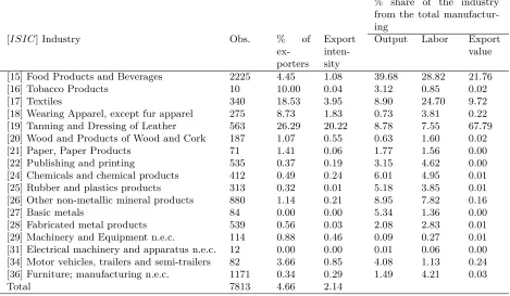
Table2presents the manufacturing size and export participation by industry defined at 2-digit ISIC classification. On average, food and beverages, textile, wearing apparels and tanning and dressing of leather products together accounted for 65% of the total employment and 58% of the total production of the Ethiopian manufacturing industry. Of these, food and beverage appears to be the most important sector producing 40% of the output value and providing jobs for 29% of the labor force in the country’s manufacturing sector. The textile industry equally employees about one third of the manufacturing labor although its contribution to the total output remains below 10%. The Ethiopian manufacturing sector is characterized by very low export performance in which only 4.7 % of firms export about 2% of the total manufacturing output. Nevertheless, the export participation largely varies across industries where tanning and leather (26%), textiles (19%) and wearing apparel (9%) are the top three export oriented sectors with higher export participation followed by food and beverage producers (4.5%). Tanning and leather industry is not only leading by export participation, but also by export intensity exporting 20% of the total output of the sector. Similar to foreign market participation rate, the gap in export intensity across sectors is significant. For example, the second top export sector, the textile industry, follows far behind the leather industry by exporting only 4% of its total output.
Table 2: Export, output and employment by 2-digit industry
% share of the industry from the total manufactur-ing
[ISIC] Industry Obs. % of
ex-porters
Export inten-sity
Output Labor Export
value
[15] Food Products and Beverages 2225 4.45 1.08 39.68 28.82 21.76
[16] Tobacco Products 10 10.00 0.04 3.12 0.85 0.02
[17] Textiles 340 18.53 3.95 8.90 24.70 9.72
[18] Wearing Apparel, except fur apparel 275 8.73 1.83 0.73 3.81 0.22
[19] Tanning and Dressing of Leather 563 26.29 20.22 8.78 7.55 67.79
[20] Wood and Products of Wood and Cork 187 1.07 0.55 0.63 1.60 0.02
[21] Paper, Paper Products 71 1.41 0.06 1.77 1.56 0.00
[22] Publishing and printing 535 0.37 0.19 3.15 4.62 0.00
[24] Chemicals and chemical products 412 0.49 0.24 6.01 4.95 0.01
[25] Rubber and plastics products 313 0.32 0.01 5.18 3.85 0.01
[26] Other non-metallic mineral products 880 1.14 0.21 8.95 7.82 0.16
[27] Basic metals 84 0.00 0.00 5.34 1.36 0.00
[28] Fabricated metal products 539 0.56 0.03 2.08 2.83 0.01
[29] Machinery and Equipment n.e.c. 114 0.88 0.46 0.09 0.27 0.01
[31] Electrical machinery and apparatus n.e.c. 12 0.00 0.00 0.01 0.06 0.00
[34] Motor vehicles, trailers and semi-trailers 82 3.66 0.85 4.08 1.13 0.24
[36] Furniture; manufacturing n.e.c. 1171 0.34 0.29 1.49 4.21 0.03
Total 7813 4.66 2.14
and input information are also excluded. This data cleaning procedure yields 2448 observations that could potentially be used in the analysis of the paper. However, since the data is unbalanced, the sample size actually used for analysis across the paper may vary depending on the method implemented.
4.2 Key Facts Established in the Data
Exporters are different
This section checks whether the data replicate the main systematic differences between exporters and non-exporters established in the literature. This is carried out by regressing various plant characteristics on an indicator variable for whether a firm exports in periodtwhile controlling for plant size, year and industry dummies. The reference group is firms that do not export in period t. The model is specified in logarithmic form, so the coefficient on export dummy captures the average premium of exporters. As all exporters are not the same, I further examine the premium of export starters, always exporters and export switchers relative to firms that never export.
Results in the first three rows of the lower panel of Table 3 present premium for the different types of exporters: always exporters, export starters and export switchers relative to never ex-porters. While always exporters employ 235% more labor than never exporters, export starters employ 192% more labor than never exporters. Export switchers and always exporters charge 70% and 20% higher price than never exporters, respectively. Starters also have 20% price premium. Nevertheless, it appears that the capital and capital intensity of always exporters is not different from never exporters. Similarly, there is no significant difference between export switchers and never exporters in terms of investment and value of sales. The general picture drawn from this analysis is that firms that export at some point in time outperform those that never export.
Price heterogeneity
The interest here is to show the extent to which prices vary across firms within an industry. Figure1plots the standard deviations (SD) and the difference between the 75th and 25th percentile of the price distribution (inter-quartile ranges) of the log of price’s of firms in a 4-digit industry. The interquartile range (IQR) is 50% or more in eleven out of eighteen sectors. However, there is variation on the dispersion of prices across sectors. Firms that produce sprits (ISIC 1551) show the lowest variation in price (about 10%) while wearing apparel manufacturers (ISIC 1810) show the highest price variation of 260%. To get a more representative idea of the spread of price, I also compute the deviations of each firm price from the industry mean. Again one can observe significant deviations from the industry mean price across industries that range from 10% in manufacturers of animal feed (ISIC 1533) to 140% in the manufacturers of wearing and apparel (ISIC 1810). The observed large within-industry price variation suggests that the use of firm revenue deflated by aggregate price as a proxy for quantity would remove an important source of heterogeneity in the estimated productivity.
0 .5 1 1.5 2 2.5
[1920]Footwear [1910]Tanning and dressing of le [1810]Wearing apparel,except fur [1730] Knitted and crocheted fab [1723] Cordage, rope, twine and [1710]Preparation of textile fib [1554]Soft drinks [1553]Beer [1552]Wines [1551] Spirits [1549]Food NEC [1544]Pasta and macaroni [1542]Sugar and confectionery [1533]Animal feed [1531]Flour [1520]Diary products [1514]Edible oil [1511]Meat production and Proces
SD of log price IQ of log price
Figure 1: Price dispersion
Price is decreasing in physical efficiency
[image:13.612.165.446.412.615.2]Table 3: Difference between exporters and non-exporters
Dep.Vars log(L) log(K) log(K/L) log(Invt) log(Invt/L) log(Sale) log(Price)
Expit 1.71*** 0.56*** 0.77*** 1.19*** 3.18*** 0.30*** 0.22**
(0.10) (0.17) (0.16) (0.42) (0.41) (0.09) (0.09)
Expalwaysi 2.35*** 0.09 0.28 1.47** 4.12*** 0.31** 0.42***
(0.14) (0.25) (0.24) (0.64) (0.62) (0.13) (0.13)
Expstarteri 1.92*** 0.28* 0.43*** 1.51*** 3.67*** 0.43*** 0.21**
(0.09) (0.17) (0.15) (0.42) (0.40) (0.09) (0.09)
Expswitcheri 1.58*** 1.05*** 1.18*** -0.24 1.54*** -0.00 0.70***
(0.08) (0.15) (0.14) (0.39) (0.37) (0.08) (0.08)
Obs. 2,448 2,448 2,448 2,448 2,448 2,448 2,288
R-squared 0.28/0.41 0.43/0.44 0.12/0.14 0.33/0.33 0.10/0.12 0.74/0.75 0.29/0.32
Note: The base line category for the results in the upper section of the table are firms that do not export in periodt. Those that never export are the baseline category in the lower part of the table. All the models control for full set of year and industry dummies. Standard errors reported in parenthesis and ***: p<1%; **: p<5%; *: p<10%.
price is decreasing in efficiency suggesting that more efficient (and thus low cost) firms charge lower prices than less efficient (high cost) firms. These results are similar to the findings of Foster et al. (2008).
−4
−2
0
2
4
6
−2 0 2 4 6 8
TFPR
95% CI Fitted values log price
−4
−2
0
2
4
6
−10 −5 0 5 10
TFPQ
[image:14.612.316.496.377.506.2]95% CI Fitted values log price
Figure 2: Price and TFP correlation
Productivity heterogeneity for both exporters and non-exporters
[image:14.612.127.493.378.505.2]exporters in food and beverage sector is driven by those firms on the 50th and above percentile of the productivity distribution. The average superior performance of non-exporters in textile and apparel sector is also driven by those at the 25th and above of the distribution. This statistics shows the existence of both high productive non-exporters and low productive exporters within a narrowly defined industry. This poses a caution on the representativeness of the average export-productivity relationship analysis.
Table 4: Productivity distribution of exporters and non-exporters
Sector Export Status Mean SD p5 p25 p50 p75 p95
Revenue based productivity (TFPR) (level)
Food and Beverage Exporters (N=98) 13.73 30.73 3.31 5.57 10.30 12.51 24.9
Non-exporters (N=1,196) 7.55 40.09 3.25 4.82 5.78 6.93 10.77
Textile and Apparel Exporters (N=87) 9.25 5.79 5.34 7.17 8.20 10.25 15.20
Non-exporters (N=509) 8.65 4.12 4.00 6.43 7.83 10.06 15.03
Leather and Footwear Exporters (N=147) 7.37 2.40 4.56 6.04 7.16 8.25 10.43
Non-exporters (N=411) 7.58 2.79 3.96 5.81 7.16 8.84 12.11
Physical productivity (TFPQ)(level)
Food and Beverage Exporters (N=98) 11.49 89.58 0.04 0.22 1.27 2.27 7.16
Non-exporters (N=1,196) 2.07 7.76 0.19 0 .55 1.16 1.55 4.74
Textile and Apparel Exporters (N=87) 4.04 8.37 0 .44 0.74 2.78 4.16 9.54
Non-exporters (N=509) 22.51 80.60 0.34 1.50 3.45 8.43 106.8
Leather and Footwear Exporters (N=147) 0.01 0.01 0. 00 0.00 0.00 0.01 0.02
Non-exporters (N=411) 0.01 0.06 0.00 0.00 0.00 0.01 0.02
TFP measures are in levels. Columns p5-p95 indicate percentiles
5 Econometric Results
5.1 Export premium
Table 5presents the export premium estimates from pooled OLS (columns 1 and 4) and fixed effect (columns 2 and 5) estimates6. Columns 1-2 show the revenue productivity export premium while columns 4-6 show the physical productivity export premium. In the OLS estimates (column 1), exporters appear to be about 20% more productive than non-exporters. The superior revenue productivity of exporters remains significant even after controlling for firm-fixed effects, though its magnitude drops to 10% (column 2). However, the result shows no significant physical productivity difference between exporters and non-exporters in both OLS and FE estimates. Intuitively, these results suggest that productivity efficiency is not the main drive for export decision and rather other sources of firm heterogeneity such as price plays crucial roles.
Considering the export premium of different types of exporters, the result shows that export starters and always exporters outperform never exporters in terms of TFPR. Specifically, always exporters show 22% export premium where as starters have 17% export premium. However switch-ers are not different from firms that never exporter (column 3). This suggests that, in quantitative terms, the export premium mainly comes from firms that always export and those that start to export. Once price heterogeneity is controlled for, the export coefficients for starters and always
6
exporters are no longer significant (column 6). Rather, export switchers appear to be 63% less efficient than never exporters. This result is the reflection of the larger price premium of switchers established in Table 3 and suggests that the inferior physical efficiency of exporters comes from the relative inefficiency of firms that switch between export and domestic markets. Furthermore, the significant drop in revenue productivity export premium in the fixed effect estimates reveals the importance of firm-specific time-invariant characteristics in bridging the gap between exporters and non-exporters.
Table 5: Productivity premium of exporters
TFPR TFPQ
Expit 0.19*** 0.10** -0.22 0.05
(0.07) (0.04) (0.24) (0.08)
Expalwaysi 0.22* -0.21
(0.12) (0.48)
Expstarter
i 0.17*** -0.36
(0.06) (0.27)
Expswitcheri 0.01 -0.64***
(0.06) (0.21)
Firm FE No Yes No No Yes No
No of firms 555 555
No observations 2,448 2,448 2,448 2,448 2,448 2,448
R-squared 0.15 0.04 0.15 0.82 0.04 0.82
Note: All the models control for log of employment and a full set of year and industry dummies. Robust standard errors in parenthesis. For OLS estimates standard errors are clustered at firm-level, ***: p<1%; **: p<5%; *: p<10%.
Table6presents the export premium of different quantiles. Columns 1 and 7 report the average coefficients estimated using OLS and fixed effects, for comparison purpose. These are similar to those reported in Table 5. The remaining columns in the upper panel of the table report results from fixed effect quantile regressions. The lower panels of the table presents results from standard cross-sectional quantile regression. For both productivity measures, the export coefficient is larger at the lower and higher quantiles, albeit it is much larger at the upper quantiles. For TFPR, for example, at the 95% quantile, the coefficient of export is over 3 times larger than the coefficient at the median. The relationship between exporting and physical productivity is positive for firms with median and above productivity level. However it is marginally significant only at the 95% quantile.
Table 6: Exporters premium at different quantiles of productivity distribution
TFPR TFPQ
FE/OLS q5 q25 q50 q75 q95 FE/OLS q5 q25 q50 q75 q95
Fixed effect quantile regression
Expit 0.10** 0.15* 0.05** 0.07*** 0.08*** 0.23** 0.05 -0.01 -0.05 0.04 0.07 0.45*
(0.04) (0.09) (0.03) (0.02) (0.03) (0.11) (0.08) (0.17) (0.05) (0.04) (0.06) (0.24)
Cross-sectional quantile regression
Expit 0.19*** 0.18** 0.07 0.12*** 0.19*** 0.55*** -0.22 -0.38** -0.48** -0.11 -0.09 0.42*
(0.07) (0.08) (0.04) (0.03) (0.07) (0.13) (0.24) (0.19) (0.20) (0.14) (0.16) (0.21)
Expalwaysi 0.22* 0.36*** 0.03 0.10** 0.20*** 0.33* -0.21 -0.26 -0.71** -0.46*** 0.19 0.53**
(0.12) (0.13) (0.06) (0.05) (0.07) (0.19) (0.48) (0.62) (0.29) (0.15) (0.28) (0.25)
Expstarteri 0.17*** 0.33*** 0.09** 0.13*** 0.14*** 0.36** -0.36 -1.36*** -1.01*** -0.03 0.10 0.16
(0.06) (0.09) (0.04) (0.03) (0.05) (0.18) (0.27) (0.23) (0.15) (0.12) (0.07) (0.27)
Expswitcheri 0.01 -0.05 -0.04 -0.02 0.01 0.39** -0.64** -0.82*** -0.86*** -0.58*** -0.36*** 0.02
(0.06) (0.12) (0.03) (0.03) (0.04) (0.15) (o.21) (0.16) (0.10) (0.15) (0.12) (0.33)
No of obs. 2,448 2,448 2,448 2,448 2,448 2,448 2,448 2,448 2,448 2,448 2,448 2,448
Columns labeled with q5-q95 represent quantiles. All the models control for log of employment and a full set of year and industry dummies. Bootstrap standard errors (100 reps) are reported in parenthesis, where ***: p<1%; **: p<5%; *: p<10%..
Taking TFPR, along the entire productivity distribution, export starters outperform non-exporters with export premium ranging from 36% (at the the 95% quantile) to 9% (at the 25% quantile). Similar pattern is observed for firms that export continuously, except at the 25% quantile where continuous exporters are not different from never exporters. Nevertheless, export switchers are not different from never exporters except for those with productivity at the upper end of the distribution.
This result is similar to the findings of Powell and Wagner (2014) where the productivity premium of exporters on the upper and lower end of the productivity distribution are larger than the premium on the median suggesting a U-shaped export-productivity links across quantiles. Considering productive efficiency, firms with some export experience are worse than those without any export experience. Evaluating at the median, for example, export starters experience 101% lower efficiency than firms that never export. Switchers also have 86% lower efficiency compared with never exporters. Nevertheless, continuously exporting firms that are at the upper quantile of the efficiency distribution enjoy 53% export premium. The overall results suggest that, productivity is more strongly related with exporting for firms with a high enough level of productivity.
5.2 self-selection
Before going to the econometric analysis of assessing the self-selection of more productive firms into foreign markets, I present the graphical trajectory of the average productivity of new exporters before and after export entry . Figures 3 shows the TFPR (on the left) and TFPQ (on the right) dynamics of new exporters and firms that never export. The horizontal axis plots a time frame where it is zero at export entry. The negative values indicate the period prior to entry while the positives are periods after entry. Thus, for new exporters the left side of the graphs deals with the self-selection while the right side captures the learning effect. For never exporters the time scale is the median years that they happen to exist in the sample. From a visual inspection of the figure, it is apparent that new exporters are more revenue productive than never exporters throughout the time windows considered and increase their TFPR in the run-up phase and after export entry. This suggests the presence of both self-selection and learning effects.
On the other hand, new exporters show lower TFPQ than never exporters both before and after export entry. A closer look at the dynamics further shows that productivity efficiency of future exporters drops one year prior to entry and continues to fall until the first year of export. It seems that their efficiency starts to recover after the first year of export experience. Though informative, the analysis so far does not take into account other factors that may affect the productivity dynamics of firms.
1.8
2
2.2
2.4
2.6
log of average revenue Productivity
−2 −1 0 1 2
time
New Exporter Never Exporter
−2.5
−2
−1.5
−1
−.5
log of average physical Productivity
−2 −1 0 1 2
time
[image:18.612.252.488.547.675.2]New Exporter Never Exporter
Table 7 presents the econometric results from equation (6) examining whether the pattern we observed in the graphs remains valid after controlling for various firm characteristics. The results show that export starters had higher TFPR than never-exporters prior to export entry suggesting high revenue firms self-select into export (columns 1-3). A closer look on the timing shows export starters outperformed since three years prior to their foreign market entry, though the highest gap is observed two years before entry. Specifically, future exporters have 23% higher TFPR premium two years prior to entry than firms that never export. The finding on the ex ante productivity difference is in line with the well-established empirical regularity in this literature that more (revenue) productive firms self-select into foreign markets. However, what is more interesting is that there is no statistically significant TFPQ difference between new exporters and never exporters prior to export entry (Columns 4-6). This suggests that productive efficiency is not the main driver behind firms decision to export instead other firm-specific demand side factors embodied in firms revenue are more important.
Table 7: Productivity difference between new exporters and never exporters prior to export entry
TFPR TFPQ
τ = 1 τ= 2 τ= 3 τ = 1 τ= 2 τ= 3
Expit0 0.15** 0.23*** 0.21** -0.44 -0.41 -0.38 (0.07) (0.08) (0.08) (0.39) (0.32) (0.35)
No observations 1,518 1,164 904 1,518 1,164 904
Of which starters 183 157 134 183 157 134
No of firms 369 277 222 369 277 222
R-squared 0.13 0.13 0.11 0.82 0.82 0.82
Note:Expit0is a dummy for export starters. Baseline category is firms that never export. τis the number of years before entry
into foreign markets. All the models control for log employment and full set of year and industry dummies. Robust standard errors clustered at firm-level in parenthesis and ***: p<1%; **: p<5%; *: p<10%.
5.3 Productivity effects of exporting
Table (8) presents the results on the productivity effect of exporting from dynamic production function estimates that directly incorporates past export status. Although the analysis is mainly based on system GMM estimates, the table also presents results from OLS, fixed effect and two-step first-difference GMM estimators for comparative purpose. The table reports tests to determine the appropriates of the GMM estimates. The first is the Hansen test of overidentifying restrictions with the null hypothesis that instruments are valid. The difference Sargan test checks the validity of the additional exclusion restrictions that arise from the level equations of the system GMM model. A further test is the Arellano-Bond test for autocorrelation of errors, with a null hypothesis of no autocorrelation (Arellano and Bond, 1991). The model is estimated using two-step GMM procedure in which the reported standard errors are robust and Windmeijer (2005) finite-sample corrected.7 All the specifications passed the overidentifying restriction test ensuring the validity
of the instruments. Similarly, the difference Sargan test confirms the validity of the additional exclusion restrictions. The rows for AR(1) and AR(2) report the p-values of Arellano and Bond test for first-order and second-order serial autocorrelation in the first-differenced residual. As expected, the test suggests high first order autocorrelation, but not second order autocorrelation in all the models. Overall, the test results suggest proper model specifications. Industry and year
7
fixed effects are controlled for in all the specifications, but the coefficients are not reported for brevity.
Columns 1 to 5 report the results using deflated firm revenue as a dependent variable. The positive and significant coefficient for lag export status suggests that previous export activity shifts the production function out. Specifically, exporting appears to increase productivity by 8% to 15%, where the lower bound is obtained from the FE estimates while the upper bound from obtained in system GMM estimates. This result supports the notion of learning effect of exporting on TFPR. Column 5 controls for the export experience of firms in addition to past export status. Export experience is statistically insignificant while the significance and sign of other variables remain the same, albeit a drop in export coefficient by 4%. This result is qualitatively and quantitatively similar to the findings of Bigsten and Gebreeyesus (2009) that use the same data and apply the same methodology. Using similar approachVan Biesebroeck (2005) finds a positive and significant effect of export with the coefficient ranging from 20% to 38% for sub-Saharan Africa firms.
[image:20.612.76.539.422.661.2]Reaffirming the evidences established by earlier studies, the main interest of this paper is to examine whether the productivity gains associated with export remains in place after price varia-tions across firms embodied in TFPR is removed. This is carried out applying the same procedure, but using quantity output as a dependent variable in the production function instead of deflated revenue. Columns 6 to 10 of Table 8 report the results for various estimators. In OLS estimates, previous export has a negative and significant coefficient. However, once firm fixed effects and potential endogeneity are addressed using FE and GMM estimators, the coefficient of lagged ex-port becomes statistically insignificant. Controlling exex-port experience in the last column does not change the results.
Table 8: The effect of export on firm’s productivity:All observations
Revenue (deflated) Quantity output
OLS FE
Diff-GMM SYS-GMM
SYS-GMM
OLS FE
Diff-GMM SYS-GMM
SYS-GMM
log(Qit−1) 0.19*** 0.10*** 0.13*** 0.15*** 0.16*** 0.65*** 0.05** 0.10** 0.22*** 0.24***
(0.02) (0.01) (0.02) (0.02) (0.02) 0.03) (0.02) (0.04) (0.04) (0.04)
log(Lit) 0.13*** 0.14*** 0.11 0.08** 0.09** -0.08** 0.10* 0.10 0.01 0.06
(0.02) (0.03) (0.08) (0.04) (0.04) (0.03) (0.05) (0.11) (0.08) (0.09)
log(Mit) 0.72*** 0.76*** 0.74*** 0.81*** 0.81*** 0.39*** 0.59*** 0.58*** 0.73*** 0.74***
(0.03) (0.02) (0.08) (0.03) (0.03) (0.04) (0.03) (0.07) (0.06) (0.06)
log(Kit) 0.01 0.01 -0.02 -0.01 -0.01 0.03* 0.03* -0.02 -0.01 -0.02
(0.01) (0.01) (0.01) (0.01) (0.01) (0.02) (0.02) (0.04) (0.03) (0.02)
Expit−1 0.13** 0.08* 0.12* 0.15** 0.11** -0.23** -0.02 0.10 0.01 0.01
(0.06) (0.05) (0.07) (0.06) (0.05) (0.11) (0.09) (0.14) (0.17) (0.12)
ExExpit -0.01 -0.09
(0.03) (0.07)
No of obs. 1841 1841 1397 1841 1841 1841 1,841 1397 1841 1841
No of firms 414 414 310 414 414 414 414 310 414 414
R-squared 0.97 0.90
P values
AR(1) 0.005 0.004 0.004 0.000 0.000 0.000
AR(2) 0.185 0.175 0.173 0.571 0.252 0.243
Hansen test of overid. 0.435 0.458 0.447 0.668 0.681 0.706
Diff-in-Hansen test 0.617 0.568 0.610 0.656 0.734 0.598
Table 9: The effect of export on firm’s productivity: Matched sample
Revenue (deflated) Quantity output
OLS FE
Diff-GMM
GMM-SYS
GMM-SYS
OLS FE
Diff-GMM
GMM-SYS
GMM-SYS
log(Qit−1) 0.41*** 0.32*** 0.08 0.37*** 0.37*** 0.76*** 0.14*** 0.04 0.63*** 0.61***
(0.07) (0.03 (0.06) (0.07) (0.08) (0.05) (0.04) (0.08) (0.08) (0.08)
log(Lit) 0.10*** 0.06 0.11 0.03 0.04 0.01 0.18 0.01 0.11 0.14
(0.03) (0.06) (0.09) 0.05) (0.04) (0.06) (0.12) (0.13) (0.12) (0.13)
log(Mit) 0.55*** 0.41*** 0.40*** 0.64*** 0.62*** 0.37*** 0.43*** 0.38*** 0.59*** 0.59***
(0.07) (0.03) (0.15) (0.09) (0.08) (0.08) (0.05) (0.14) (0.13) (0.13)
log(Kit) -0.00 0.05** 0.05 0.02 0.03 -0.01 -0.00 0.02 -0.01 -0.01
(0.02) (0.02) (0.03) (0.03) (0.02) (0.03) (0.04) (0.04) (0.05) (0.05)
Expit−1 0.19*** 0.15*** 0.19* 0.19** 0.14* -0.06 0.15 0.09 -0.05 -0.09
(0.05) (0.05) (0.10) (0.08) (0.08) (0.08) (0.09) (0.16) (0.14) (0.15)
ExExpit 0.01 0.01
(0.02) (0.03)
No of obs. 657 657 538 657 657 657 657 538 657 657
No of firms 192 192 160 192 192 192 192 160 192 192
R-squared 0.96 0.92
P values
AR(1) 0.010 0.004 0.005 0.046 0.026 0.026
AR(2) 0.623 0.335 0.333 0.400 0.450 0.426
Hansen test of overid. 0.990 0.321 0.416 0.989 0.228 0.333
Diff-in-Hansen test 0.971 0.159 0.252 0.974 0.336 0.307
Note: The instruments for the first difference in the GMM estimators are from first to third lag for inputs and second and third lag for output, export status and export experience. The standard errors are robust finite sample corrected on two-step estimates where ***: p<1%; **: p<5%; *: p<10%. The P values of the different tests are presented at the end of the table. All the models control for full set of year and industry dummies.
The input coefficients deserve some comments. In all specifications, the lag output coefficient is positive and significant suggesting the persistence of productivity. As expected, the coefficient of material is positive and significant despite the output measure used. Although the labor coefficient has the expected sign and significance in the revenue production function, surprisingly it is either negative or at best statistically insignificant in the quantity based production function. One possible explanation for this insignificant coefficients for labor could be associated with the fact that this production function controls output price bias only leaving aside some possible heterogeneity in input prices. This issue is addressed in the robustness checks. Similarly, the estimated coefficient for capital in the preferred estimators has the wrong sign, although it is not significant. One possible explanation can be that the available capital stock data used in the estimation may not be good enough to identify variations in the flow of capital service used in the production process of firms. The insignificant capital coefficient is consistent with the general experience of studies that proxy capital service with capital stock measure. Harper(1999), for example, pointed out that the use of capital stock as a substitute for capital service would more likely underestimate the contribution of capital in the production process. Nevertheless, the available data do not have information to estimate capital service.
shift in the productivity, depending on the estimator used. However, when price effects is removed using quantity output, the effect of export on productivity disappears (Columns 6 to 10). This is similar to the result in the above subsection using the entire (matched and unmatched) sample. To sum up, this section examines the effect of export on productivity allowing for endogenous inputs and export while controlling for price heterogeneity and self-selection of more productive firms into export. Despite the estimator used, the results support the empirical regularity in the export-productivity literature (especially in developing countries) that firms improve (revenue) productivity due to export participation. However, when price heterogeneity is controlled using physical output, the effect of exporting on productivity is no longer significant suggesting that price could be the main mechanism through which export affects the measured productivity.
5.4 Robustness Checks
This section presents a number of checks if the main results of learning effects are robust to (i) a detail classification of exporters, (ii) the use of alternative measure of quantity output and (iii) controlling for input price heterogeneity in addition to output price heterogeneity. The results above suggest that exporting has a positive effect on revenue productivity, but not on efficiency. These results were obtained using all the types of exporters without differentiating export starters, continuous exporters and export switchers. The main concern here is that such analysis may compare continuous exporters themselves at different periods and the results may be influenced by occasional exporters. Thus, the first check involves verifying the sensitivity of the results to considering export starters and never exporters, disregarding export switchers and continuous exporters. To that end, I repeat the learning effect analysis applying preferred system GMM estimator, but restricting the sample to export starters and never exporters.
Columns 1 and 2 of Table 10 reports the results. To address the potential selection bias, I construct a matched sample by estimating propensity score using equation8. However, unlike the previous matching procedure, the dependent variable in the current case is a dummy equals one if the firm is export starter and zero if it is never-exporter. Thus, export starters are matched with firms that never export, but have a comparable propensity to start exporting as firms that started exporting. The results of the propensity to start exporting are reported in Column 2 of the Table in Appendix A.2. Columns 3 and 4 of Table 10 report the learning effect results obtained on the matched sample. The coefficients of the lag of export status appear to be positive and significant in columns 1 and 4 suggesting the presence of learning effect on revenue productivity. On the other hand, export starters show a decrease in physical efficiency after entering into foreign markets, albeit at 10 % level of significance (columns 2 and 4). These results corroborate the finding that the effect of exporting on firm performance comes through price effect. Nevertheless, comparing these results with results in Tables 8 and 9 suggests that the gains of exporting on revenue productivity is substantially larger for export starters than the whole group of exporters while export starters appear to be less efficient compared with firms that have never participated in foreign markets.
Table 10: The effect of exporting: robustness checks
All sample Matched Sample Input price bias corrected
Dep. var Revenue Quantity Revenue Quantity QuantityR Quantity QuantityR
log(Qit−1) 0.13*** 0.25*** 0.28*** 0.34** 0.25*** 0.33*** 0.32***
(0.02) (0.05) (0.08) (0.16) (0.04) (0.05) (0.05)
log(Lit) 0.10** 0.04 0.21*** 0.22** 0.04 0.28*** 0.32***
(0.04) (0.08) (0.06) (0.11) (0.10) (0.09) (0.09)
log(Mit) 0.80*** 0.69*** 0.58*** 0.64** 0.70**** 0.36*** 0.35***
(0.03) (0.07) (0.10) (0.20) (0.07) (0.05) (0.05)
log(Kit) 0.00 0.01 0.01 0.08** -0.02 -0.01 -0.02
(0.01) (0.03) (0.02) (0.04) (0.03) (0.03) (0.03)
Expit−1 0.26** -0.68* 0.30*** -0.26* -0.07 -0.08 -0.14
(0.13) (0.36) (0.09) (0.14) (0.17) (0.16) (0.16)
No of obs. 1518 1518 262 262 1841 1841 1841
No of firms 369 369 108 108 414 414 414
P values
AR(1) 0.014 0.000 0.069 0.084 0.000 0.000 0.000
AR(2) 0.189 0.231 0.404 0.726 0.273 0.482 0.426
Hansen test of overid. 0.741 0.695 1.000 1.000 0.481 0.307 0.308
Diff-in-Hansen test 0.704 0.821 1.000 1.000 0.528 0.601 0.463
Note: The instruments for the first difference in the GMM estimators are first lag and earlier for inputs and second lag and earlier for output, export status and export experience. The standard errors are robust finite sample corrected on two-step estimates where ***: p<1%; **: p<5%; *: p<10%. The P values of the different tests are presented at the end of the table. All the models control for full set of year and industry dummies.
using sales deflated by firm-level price: exporting firms do not increase their physical productivity after entry into foreign markets.
6 Conclusion
This paper re-examines the causal effects of exporting on productivity taking into account price differences across firms. Empirical studies for a large number of countries establish that exporters are more productive than non-exporters and explain this evidence as a self-selection into export and (or) learning effect from exporting. Similarly, studies in the context of African firms find similar results. However, in most studies productivity is estimated from a revenue based production function where firm output is measured by revenue (deflated by industry average price) instead of quantity as data on physical output is rarely available. The resulting productivity therefore picks up price differences across firms in addition to efficiency differences. On the other hand, a more recent literature indicates that exporters charge higher prices than non-exporters as they produce higher quality products. This in turn makes it difficult to know whether exporters are actually more productive or they simply charge higher prices for their output than non-exporters. Furthermore, it obscures the channel through which participation in foreign markets affects firm’s overall performance.
This paper exploits a rich data on quantity and prices on Ethiopian firms in the period 1996-2005. The empirical strategy involves splitting the price components that are confound in the traditional revenue-based measures of productivity and examines its implication on the estimated relationship between export and productivity. This paper differs from previous studies in this literature as it does not focus on the the relationship between exporting and productivity per se but the the effects of price heterogeneity in shaping this relationship.
The main results of the paper show that exporters are more productive than non-exporters in terms of revenue based productivity and this is explained by both self-selection and learning effects. These results are standard in the literature. Interestingly, correcting for price heterogeneity leads to an insignificant relationship between exporting and productivity. Specifically, when focusing on quantity-based measures of productivity, exporters appear to be not different from non-exporters either before and after export entry. Further evidence shows that price is increasing in revenue productivity and decreasing in physical productivity and on average exporters charge higher prices than non-exporters. Looking at the entire distribution of productivity, the export premium for firms at different points of productivity distribution differ from the premium at the mean of the produc-tivity distribution. Specifically, exporters show higher revenue producproduc-tivity across all quantiles, but the premium are larger at the lower and upper end of the productivity distribution suggesting U-shaped export-productivity links across quantiles. Nevertheless, exporters are not different from non-exporters almost throughout the entire physical productivity distribution.
Acknowledgment
A Appendix
Appendix A.1 - Variables description and data cleaning Production inputs
Labor (L) is computed as the sum of permanent employees and year-equivalent temporary workers. Capital stock (K) is measured using the reported net book value of assets at the beginning of the year. Intermediate input (M) is measured as the sum of plant expenditures on raw materials and energy. The real values of raw material and energy are obtained by deflating their nominal values using their respective deflator obtained from CSA before they are added up together.
Output and Productivity
Two versions of TFP measures are estimated using two measures of output. First, firm-level sales revenue deflated by industry average price index obtained from CSA. The fact that this output measures firms deflated revenue, the resulting productivity is termed as revenue TFP (TFPR) as inFoster et al. (2008). Second, qunatity output is constructed by dividing firm-level sales by firm-level price. This measure clearly accounts for price differences across firms and the resulting productivity captures the “true” productivity of firms that measure the quantity output produced per composition of inputs. The productivity estimated using this output is therefore referred asphysical TFP or physical efficiency (TFPQ). To check the robustness of the results based on TFPQ, I aggregate reported product-level quantity output to construct firm-level quantity (QuantityR). Then this quantity measure is used to estimate an alternative productivity measure (TFPQr). Nevertheless, estimating quantity based productivity using the available information involves a number of data cleaning procedures. First, firms even in the same industry report their quantity output in different measurement units. For example, in beverage industry, while some firms use litre, others use barrel or hectolitre. In order to reduce measurement errors, therefore, the reported quantities are standardized in the same unit. Second, some of the products are defined imprecisely as “other products” and for these products there is no information on the unit of measurement. The third problem is missing quantity data for some products listed by firms. On the other hand, as it is typical in many data sets, there is no information regards with input use in producing each product of the firm. To address this issue, I apply a proportionality principle to weight inputs when estimating productivity using the reported quantity. Specifically, denote the total sales value of products that firm i provides quantity information byVitq and the total sales value of
the firm byVit, the inputs (X= k, l, m) are adjusted as follows
xit=ln
Xit
Vitq
Vit
(A.1)
Firm specific prices
Firm-level output price is constructed using product-level quantity and sales value information reported by firms. Denote the standardized quantity sales of producthof firmiat timetbyQhitand the corresponding
sales value of the product byVhit. First the price of producthis computed as
Phit=
Vhit
Qhit
(A.2)
Then firm-level price is computed as a weighted value of the prices of the products that the firm produces:
Pit= n
X
h=1
Phit
V
hit
Vit
(A.3)