Learning Non-linear Features for Machine Translation Using Gradient
Boosting Machines
Kristina Toutanova
Microsoft Research Redmond, WA 98502 [email protected]
Byung-Gyu Ahn∗
Johns Hopkins University Baltimore, MD 21218
Abstract
In this paper we show how to auto-matically induce non-linear features for machine translation. The new features are selected to approximately maximize a BLEU-related objective and decompose on the level of local phrases, which guar-antees that the asymptotic complexity of machine translation decoding does not in-crease. We achieve this by applying gra-dient boosting machines (Friedman, 2000) to learn new weak learners (features) in the form of regression trees, using a differen-tiable loss function related to BLEU. Our results indicate that small gains in perfor-mance can be achieved using this method but we do not see the dramatic gains ob-served using feature induction for other important machine learning tasks.
1 Introduction
The linear model for machine translation (Och and Ney, 2002) has become the de-facto standard in the field. Recently, researchers have proposed a large number of additional features (TaroWatan-abe et al., 2007; Chiang et al., 2009) and param-eter tuning methods (Chiang et al., 2008b; Hop-kins and May, 2011; Cherry and Foster, 2012) which are better able to scale to the larger pa-rameter space. However, a significant feature en-gineering effort is still required from practition-ers. When a linear model does not fit well, re-searchers are careful to manually add important feature conjunctions, as for example, (Daum´e III and Jagarlamudi, 2011; Clark et al., 2012). In the related field of web search ranking, automatically learned non-linear features have brought dramatic improvements in quality (Burges et al., 2005; Wu
∗
This research was conducted during the author’s intern-ship at Microsoft Research
et al., 2010). Here we adapt the main insights of such work to the machine translation setting and share results on two language pairs.
Some recent works have attempted to relax the linearity assumption on MT features (Nguyen et al., 2007), by defining non-parametric models on complete translation hypotheses, for use in an n-best re-ranking setting. In this paper we develop a framework for inducing non-linear features in the form of regression decision trees, which de-compose locally and can be integrated efficiently in decoding. The regression trees encode non-linear feature combinations of the original fea-tures. We build on the work by Friedman (2000) which shows how to induce features to minimize any differentiable loss function. In our applica-tion the features are regression decision trees, and the loss function is the pairwise ranking log-loss from thePROmethod for parameter tuning (Hop-kins and May, 2011). Additionally, we show how to design the learning process such that the in-duced features are local on phrase-pairs and their language model and reordering context, and thus can be incorporated in decoding efficiently.
Our results using re-ranking on two language pairs show that the feature induction approach can bring small gains in performance. Overall, even though the method shows some promise, we do not see the dramatic gains that have been seen for the web search ranking task (Wu et al., 2010). Fur-ther improvements in the original feature set and the induction algorithm, as well as full integration in decoding are needed to potentially result in sub-stantial performance improvements.
2 Feature learning using gradient boosting machines
In the linear model for machine translation, the scores of translation hypotheses are weighted sums of a set of input features over the hypotheses.
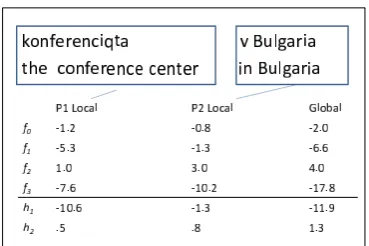
Figure 1: A Bulgarian source sentence (meaning ”the conference in Bulgaria”, together with a candidate transla-tion. Local and global features for the translation hypoth-esis are shown. f0=smoothed relative frequency estimate
of logp(s|t); f1=lexical weighting estimate of logp(s|t);
f2=joint count of the phrase-pair;f3=sum of language model
log-probabilities of target phrase words given context.
For a set of featuresf1(h), . . . , fL(h)and weights
for these features λ1, . . . , λL, the hypothesis
scores are defined as: F(h) = ∑l=1...Lλlfl(h).
In current state-of-the-art models, the features
fl(h) decompose locally on phrase-pairs (with
language model and reordering context) inside the hypotheses. This enables hypothesis recombina-tion during machine translarecombina-tion decoding, leading to faster and more accurate search. As an exam-ple, Figure 1 shows a Bulgarian source sentence (spelled phonetically in Latin script) and a can-didate translation. Two phrase-pairs are used to compose the translation, and each phrase-pair has a set of local feature function values. A mini-mal set of four features is shown, for simplicity. We can see that the hypothesis-level (global) fea-ture values are sums of phrase-level (local) feafea-ture values. The score of a translation given feature weightsλcan be computed either by scoring the phrase-pairs and adding the scores, or by scoring the complete hypothesis by computing its global feature values. The local feature values do look at some limited context outside of a phrase-pair, to compute language model scores and re-ordering scores; therefore we say that the features are de-fined on phrase-pairs in context.
We start with such a state-of-the-art linear model with decomposable features and show how we can automatically induce additional features. The new features are also locally decomposable, so that the scores of hypotheses can be computed as sums of phrase-level scores. The new local phrase-level features are non-linear combinations of the original phrase-level features.
Figure 2: Example of two decision tree features. The left decision tree has linear nodes and the right decision tree has constant nodes.
2.1 Form of induced features
We will use the example in Figure 1 to introduce the form of the new features we induce and to give an intuition of why such features might be useful. The new features are expressed by regression de-cision trees; Figure 2 shows two examples.
One intuition we might have is that, if a phrase pair has been seen very few times in the training corpus (for example, the first phrase pair P1 in the Figure has been seen only one timef2 = 1), we would like to trust its lexical weighting channel model score f1 more than its smoothed relative-frequency channel estimate f0. The first
regres-sion tree feature h1 in Figure 2 captures this in-tuition. The feature value for a phrase-pair of this feature is computed as follows: if f2 ≤ 2, then h1(f0, f1, f2, f3) = 2 × f1; otherwise,
h1(f0, f1, f2, f3) = f1. The effect of this new feature h1 is to boost the importance of the lexi-cal weighting score for phrase-pairs of low joint count. More generally, the regression tree fea-tures we consider have either linear or constant leaf nodes, and have up to 8 leaves. Deeper trees can capture more complex conditions on several input feature values. Each non-leaf node performs a comparison of some input feature value to a threshold and each leaf node (for linear nodes) re-turns the value of some input feature multiplied by some factor. For a given regression tree with linear nodes, all leaf nodes are expressions of the same input feature but have different coefficients for it (for example, both leaf nodes of h1 return affine functions of the input featuref1). A
[image:2.595.348.485.60.135.2]Having introduced the form of the new features we learn, we now turn to the methodology for in-ducing them. We apply the framework of gradient boosting for decision tree weak learners (Fried-man, 2000). To define the framework, we need to introduce the original input features, the differ-entiable loss function, and the details of the tree growing algorithm. We discuss these in turn next.
2.2 Initial features
Our baseline MT system uses relative frequency and lexical weighting channel model weights, one or more language models, distortion penalty, word count, phrase count, and multiple lexicalized re-ordering weights, one for each distortion type. We have around 15 features in thisbase feature set. We further expand the input set of features to in-crease the possibility that useful feature combi-nations could be found by our feature induction method. The large feature set contains around 190 features, including source and target word count features, joint phrase count, lexical weight-ing scores accordweight-ing to alternative word-alignment model ran over morphemes instead of words, in-dicator lexicalized features for insertion and dele-tion of the top15words in each language, cluster-based insertion and deletion indicators using hard word clustering, and cluster based signatures of phrase-pairs. This is the feature set we use as a basis for weak learner induction.
2.3 Loss function
We use a pair-wise ranking log-loss as in the PROparameter tuning method (Hopkins and May, 2011). The loss is defined by comparing the model scores of pairs of hypotheses hi and hj where
the BLEU score of the first hypothesis is greater than the BLEU score of the second hypothesis by a specified threshold.1
We denote the sentences in a corpus as
s1, s2, . . . , sN. For each sentence sn, we
de-note the ordered selected pairs of hypotheses as [hni1, hnj1], . . . ,[hniK, hnjK]. The loss-function Ψis defined in terms of the hypothesis model scores 1In our implementation, for each sentence, we sample
10,000 pairs of translations and accept a pair of transla-tions for use with probability proportional to the BLEUscore
difference, if that difference is greater than the threshold of 0.04. The topK = 100orK= 300hypothesis pairs with the largest BLEUdifference are selected for computation of
the loss. We compute sentence-level BLEUscores by add-α
smoothing of the match counts for computation of n-gram precision. The αandK parameters are chosen via cross-validation.
1: F0(x) = arg minλΨ(F(x, λ)) 2: form= 1toM do
3: yr = −[∂∂FΨ(F(x(rx)))]F(x)=Fm−1(x), r =
1. . . R
[image:3.595.311.524.63.173.2]4: αm= arg minα,β∑Rr=1[yr−βh(xi;α)]2 5: ρm= arg minρΨ(Fm−1(x) +ρh(x;αm) 6: Fm(x) =Fm−1(x) +ρmh(x;αm) 7: end for
Figure 3: A gradient boosting algorithm for local feature functions.
F(h) as follows: ∑n=1...N∑k=1...Klog(1 +
eF(hnjk)−F(hnik)).
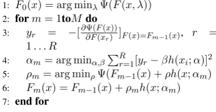
The idea of the gradient boosting method is to induce additional features by computing a func-tional gradient of the target loss function and itera-tively selecting the next weak learner (feature) that is most parallel to the negative gradient. Since we want to induce features such that the hypothesis scores decompose locally, we need to formulate our loss function as a function of local phrase-pair in context scores. Having the model scores de-compose locally means that the scores of hypothe-ses F(h) decompose as F(h) = ∑pr∈hF(pr)),
where bypr ∈hwe denote the enumeration over
phrase pairs in context that are parts ofh. Ifxr
de-notes the input feature vector for a phrase-pair in contextpr, the score of this phrase-pair can be
ex-pressed asF(xr). Appendix A expresses the
pair-wise log-loss as a function of the phrase scores. We are now ready to introduce the gradient boosting algorithm, summarized in Figure 3. In the first step of the algorithm, we start by set-ting the phrase-pair in context scoring function
F0(x)as a linear function of the input feature val-ues, by selecting the feature weights λ to
min-imize the PRO loss Ψ(F0(x)) as a function of
λ. The initial scores have the form F0(x) =
∑
l=1...Lλlfl(x).This is equivalent to using the
(Hopkins and May, 2011) method of parameter tuning for a fixed input feature set and a linear model. We used LBFGS for the optimization in Line 1. Then we iterate and induce a new de-cision tree weak learnerh(x;αm) like the
exam-ples in Figure 2 at each iteration. The parame-ter vectorsαm encode the topology and
Language Train Dev-Train Dev-Select Test
Chs-En 999K NIST02+03 2K NIST05
[image:4.595.88.274.61.90.2]Fin-En 2.2M 12K 2K 4.8K
Table 1: Data sets for the two language pairs Chinese-English and Finnish-Chinese-English.
Chs-En Fin-En
Features Tune Dev-Train Test Dev-Train Test
base MERT 31.3 30.76 49.8 51.31
base PRO 31.1 31.16 49.7 51.56
large PRO 31.8 31.44 49.8 51.77 boost-global PRO 31.8 31.30 50.0 51.87 boost-local PRO 31.8 31.44 50.1 51.95
Table 2: Results for the two language pairs using different weight tuning methods and feature sets.
h(x;αm) is induced, it is treated as new feature
and a linear coefficient ρm for that feature is set
by minimizing the loss as a function of this pa-rameter (Line 5). The new model scores are set as the old model scores plus a weighted contribution from the new feature (Line 6). At the end of learn-ing, we have a linear model over the input features and additional decision tree features. FM(x) =
∑
l=1...Lλlfl(x) +∑m=1...Mρmh(x;αm). The
most time-intensive step of the algorithm is the se-lection of the next decision tree h. This is done
by first computing the functional gradient of the loss with respect to the phrase scoresF(xr)at the
point of the current model scoresFm−1(xr).
Ap-pendix A shows a derivation of this gradient. We then induce a regression tree using mean-square-error minimization, setting the direction given by the negative gradient as a target to be predicted us-ing the features of each phrase-pair in context in-stance. This is shown as the setting of theαm
pa-rameters by mean-squared-error minimization in Line 4 of the algorithm. The minimization is done approximately by a standard greedy tree-growing algorithm (Breiman et al., 1984). When we tune weights to minimize the loss, such as the weights
λof the initial features, or the weights ρm of
in-duced learners, we also include an L2 penalty on the parameters, to prevent overfitting.
3 Experiments
We report experimental results on two language pairs: Chinese-English, and Finnish-English. Ta-ble 1 summarizes statistics about the data. For each language pair, we used a training set (Train) for extracting phrase tables and language models, a Dev-Train set for tuning feature weights and in-ducing features, a Dev-Select set for selecting hy-perparameters ofPROtuning and selecting a
stop-ping point and other hyperparameters of the boost-ing method, and a Test set for reportboost-ing final re-sults. For Chinese-English, the training corpus consists of approximately one million sentence pairs from the FBIS and HongKong portions of the LDC data for the NIST MT evaluation and the Dev-Train and Test sets are from NIST competi-tions. The MT system is a phrasal system with a 4-gram language model, trained on the Xinhua por-tion of the English Gigaword corpus. The phrase table has maximum phrase length of 7 words on either side. For Finnish-English we used a data-set from a technical domain of software manuals. For this language pair we used two language mod-els: one very large model trained on billions of words, and another language model trained from the target side of the parallel training set. We re-port performance using the BLEU-SBPmetric pro-posed in (Chiang et al., 2008a). This is a vari-ant of BLEU (Papineni et al., 2002) with strict brevity penalty, where a long translation for one sentence can not be used to counteract the brevity penalty for another sentence with a short transla-tion. Chiang et al. (2008a) showed that this metric overcomes several undesirable properties of BLEU and has better correlation with human judgements. In our experiments with different feature sets and hyperparameters we observed more stable results and better correlation of Dev-Train, Dev-Select, and Test results using BLEU-SBP. For our exper-iments, we first trained weights for thebase fea-ture sets described in Section 2.2 using MERT. We then decoded the Dev-Train, Dev-Select, and Test datasets, generating 500-best lists for each set. All results in Table 2 report performance of re-ranking on these 500-best lists using different feature sets and parameter tuning methods.
[image:4.595.76.287.133.193.2]addition to learning locally decomposable features
boost-local, we also implementedboost-global, where we are learning combinations of the global feature values and lose decomposability. The fea-tures learned by boost-global can not be com-puted exactly on partial hypotheses in decoding and thus this method has a speed disadvantage, but we wanted to compare the performance of boost-local andboost-global on n-best list re-ranking to see the potential accuracy gain of the two meth-ods. We see that boost-localis slightly better in performance, in addition to being amenable to ef-ficient decoder integration.
The gradient boosting results are mixed; for Finnish-English, we see around .2 gain of the
boost-local model over the large feature set. There is no improvement on Chinese-English, and the boost-global method brings slight degrada-tion. We did not see a large difference in perfor-mance among models using different decision tree leaf node types and different maximum numbers of leaf nodes. The selected boost-local model for FIN-ENU used trees with maximum of 2 leaf nodes and linear leaf values; 25 new features were induced before performance started to degrade on the Dev-Select set. The induced features for Finnish included combinations of language model and channel model scores, combinations of word count and channel model scores, and combina-tions of channel and lexicalized reordering scores. For example, one feature increases the contribu-tion of the relative frequency channel score for phrases with many target words, and decreases the channel model contribution for shorter phrases.
The best boost-local model for Chs-Enu used trees with a maximum of 2 constant-values leaf nodes, and induced 24 new tree features. The fea-tures effectively promoted and demoted phrase-pairs in context based on whether an input fea-ture’s value was smaller than a determined cutoff. In conclusion, we proposed a new method to induce feature combinations for machine transla-tion, which do not increase the decoding complex-ity. There were small improvements on one lan-guage pair in a re-ranking setting. Further im-provements in the original feature set and the in-duction algorithm, as well as full integration in de-coding are needed to result in substantial perfor-mance improvements.
This work did not consider alternative ways of generating non-linear features, such as taking
products of two or more input features. It would be interesting to compare such alternatives to the regression tree features we explored.
References
Leo Breiman, Jerome Friedman, Charles J. Stone, and R.A. Olshen. 1984. Classification and Regression Trees. Chapman and Hall.
Chris Burges, Tal Shaked, Erin Renshaw, Matt Deeds, Nicole Hamilton, and Greg Hullender. 2005. Learn-ing to rank usLearn-ing gradient descent. InICML.
Colin Cherry and George Foster. 2012. Batch tuning strategies for statistical machine translation. In HLT-NAACL.
David Chiang, Steve DeNeefe, Yee Seng Chan, and Hwee Tou Ng. 2008a. Decomposability of trans-lation metrics for improved evaluation and efficient algorithms. InEMNLP.
David Chiang, Yuval Marton, and Philp Resnik. 2008b. Online large margin training of syntactic and struc-tural translation features. InEMNLP.
D. Chiang, W. Wang, and K. Knight. 2009. 11,001 new features for statistical machine translation. In
NAACL.
Jonathan Clark, Alon Lavie, and Chris Dyer. 2012. One system, many domains: Open-domain statisti-cal machine translation via feature augmentation. In
AMTA.
Hal Daum´e III and Jagadeesh Jagarlamudi. 2011. Do-main adaptation for machine translation by mining unseen words. InACL.
Jerome H. Friedman. 2000. Greedy function approx-imation: A gradient boosting machine. Annals of Statistics, 29:1189–1232.
Mark Hopkins and Jonathan May. 2011. Tuning as ranking. InEMNLP.
Patrick Nguyen, Milind Mahajan, and Xiaodong He. 2007. Training non-parametric features for statis-tical machine translation. In Second Workshop on Statistical Machine Translation.
Franz Josef Och and Hermann Ney. 2002. Discrimina-tive training and maximum entropy models for sta-tistical machine translation. InACL.
Kishore Papineni, Salim Roukos, Todd Ward, and Wei-Jing Zhu. 2002. BLEU: a method for automatic
evaluation of machine translation. InACL.
Qiang Wu, Christopher J. Burges, Krysta M. Svore, and Jianfeng Gao. 2010. Adapting boosting for infor-mation retrieval measures. Information Retrieval, 13(3), June.
4 Appendix A: Derivation of derivatives
Here we express the loss as a function of phrase-level in context scores and derive the derivative of the loss with respect to these scores.
Let us number all phrase-pairs in context in all hypotheses in all sentences as p1, . . . , pR and
denote their input feature vectors as x1, . . . ,xR.
We will use F(pr) and F(xr)
interchange-ably, because the score of a phrase-pair in context is defined by its input feature vec-tor. The loss Ψ(F(xr)) is expressed as follows:
∑N
n=1
∑K
k=1log(1 +e ∑
pr∈hn
jkF(xr)−
∑
pr∈hn
ikF(xr)).
Next we derive the derivatives of the loss Ψ(F(x))with respect to the phrase scores. Intu-itively, we are treating the scores we want to learn as parameters for the loss function; thus the loss function has a huge number of parameters, one for each instance of each phrase pair in context in each translation. We ask the loss function if these scores could be set in an arbitrary way, what di-rection it would like to move them in to be mini-mized. This is the direction given by the negative gradient.
Each phrase-pair in contextproccurs in exactly
one hypothesis h in one sentence. It is possible
that two phrase-pairs in context share the same set of input features, but for ease of implementation and exposition, we treat these as different train-ing instances. To express the gradient with respect toF(xr)we therefore need to focus on the terms
of the loss from a single sentence and to take into account the hypothesis pairs[hj,k, hi,k]where the
left or the right hypothesis is the hypothesish
con-taining our focus phrase pair pr. ∂Ψ(∂FF(x(rx))) is
ex-pressed as:
= ∑k:h=h
ik−
e ∑
pr∈hn jkF(xr)−
∑
pr∈hn ikF(xr)
1+e ∑
pr∈hn jkF(xr)−
∑
pr∈hn ikF(xr)
+ ∑k:h=h
jk
e ∑
pr∈hn jkF(xr)−
∑
pr∈hn ikF(xr)
1+e ∑
pr∈hn jkF(xr)−
∑
pr∈hn ikF(xr)
Since in the boosting step we induce a deci-sion tree to fit the negative gradient, we can see that the feature induction algorithm is trying to in-crease the scores of phrases that occur in better