Improved Bayesian Logistic Supervised Topic Models
with Data Augmentation
Jun Zhu, Xun Zheng, Bo Zhang
Department of Computer Science and Technology
TNLIST Lab and State Key Lab of Intelligent Technology and Systems Tsinghua University, Beijing, China
{dcszj,dcszb}@tsinghua.edu.cn; [email protected]
Abstract
Supervised topic models with a logistic likelihood have two issues that potential-ly limit their practical use: 1) response variables are usually over-weighted by document word counts; and 2) existing variational inference methods make strict mean-field assumptions. We address these issues by: 1) introducing a regularization constant to better balance the two parts based on an optimization formulation of Bayesian inference; and 2) developing a simple Gibbs sampling algorithm by intro-ducing auxiliary Polya-Gamma variables and collapsing out Dirichlet variables. Our augment-and-collapse sampling algorithm has analytical forms of each conditional distribution without making any restrict-ing assumptions and can be easily paral-lelized. Empirical results demonstrate sig-nificant improvements on prediction per-formance and time efficiency.
1 Introduction
As widely adopted in supervised latent Dirichlet allocation (sLDA) models (Blei and McAuliffe, 2010; Wang et al., 2009), one way to improve the predictive power of LDA is to define a like-lihood model for the widely available document-level response variables, in addition to the likeli-hood model for document words. For example, the logistic likelihood model is commonly used for bi-nary or multinomial responses. By imposing some priors, posterior inference is done with the Bayes’ rule. Though powerful, one issue that could limit the use of existing logistic supervised LDA models is that they treat the document-level response vari-able as one additional word via a normalized like-lihood model. Although some special treatment is carried out on defining the likelihood of the single
response variable, it is normally of a much small-er scale than the likelihood of the usually tens or hundreds of words in each document. As noted by (Halpern et al., 2012) and observed in our ex-periments, this model imbalance could result in a weak influence of response variables on the topic representations and thus non-satisfactory predic-tion performance. Another difficulty arises when dealing with categorical response variables is that the commonly used normal priors are no longer conjugate to the logistic likelihood and thus lead to hard inference problems. Existing approaches re-ly on variational approximation techniques which normally make strict mean-field assumptions.
To address the above issues, we present two im-provements. First, we present a general frame-work of Bayesian logistic supervised topic models with a regularization parameter to better balance response variables and words. Technically, instead of doing standard Bayesian inference via Bayes’ rule, which requires a normalized likelihood mod-el, we propose to do regularized Bayesian infer-ence (Zhu et al., 2011; Zhu et al., 2013b) via solv-ing an optimization problem, where the posterior regularization is defined as an expectation of a l-ogistic loss, a surrogate loss of the expected mis-classification error; and a regularization parame-ter is introduced to balance the surrogate classifi-cation loss (i.e., the response log-likelihood) and the word likelihood. The general formulation sub-sumes standard sLDA as a special case.
Second, to solve the intractable posterior infer-ence problem of the generalized Bayesian logis-tic supervised topic models, we present a simple Gibbs sampling algorithm by exploring the ideas of data augmentation (Tanner and Wong, 1987; van Dyk and Meng, 2001; Holmes and Held, 2006). More specifically, we extend Polson’s method for Bayesian logistic regression (Polson et al., 2012) to the generalized logistic supervised topic models, which are much more
ing due to the presence of non-trivial latent vari-ables. Technically, we introduce a set of Polya-Gamma variables, one per document, to refor-mulate the generalized logistic pseudo-likelihood model (with the regularization parameter) as a s-cale mixture, where the mixture component is con-ditionally normal for classifier parameters. Then, we develop a simple and efficient Gibbs sampling algorithms with analytic conditional distribution-s without Metropolidistribution-s-Hadistribution-stingdistribution-s accept/reject distribution-stepdistribution-s. For Bayesian LDA models, we can also explore the conjugacy of the Dirichlet-Multinomial prior-likelihood pairs to collapse out the Dirichlet vari-ables (i.e., topics and mixing proportions) to do collapsed Gibbs sampling, which can have better mixing rates (Griffiths and Steyvers, 2004). Final-ly, our empirical results on real data sets demon-strate significant improvements on time efficiency. The classification performance is also significantly improved by using appropriate regularization pa-rameters. We also provide a parallel implementa-tion with GraphLab (Gonzalez et al., 2012), which shows great promise in our preliminary studies.
The paper is structured as follows. Sec. 2 intro-duces logistic supervised topic models as a general optimization problem. Sec. 3 presents Gibbs sam-pling algorithms with data augmentation. Sec. 4 presents experiments. Sec. 5 concludes.
2 Logistic Supervised Topic Models
We now present the generalized Bayesian logistic supervised topic models.
2.1 The Generalized Models
We consider binary classification with a training setD ={(wd, yd)}Dd=1, where the response vari-able Y takes values from the output space Y = {0,1}. A logistic supervised topic model consists of two parts — an LDA model (Blei et al., 2003) for describing the words W = {wd}Dd=1, where wd = {wdn}Nn=1d denote the words within docu-mentd, and a logistic classifier for considering the
supervising signaly={yd}Dd=1. Below, we
intro-duce each of them in turn.
LDA: LDA is a hierarchical Bayesian model that posits each document as an admixture ofK
topics, where each topicΦk is a multinomial
dis-tribution over aV-word vocabulary. For document d, the generating process is
1. draw a topic proportionθd∼Dir(α)
2. for each wordn= 1,2, . . . , Nd:
(a) draw a topic1z
dn ∼Mult(θd)
(b) draw the wordwdn ∼Mult(Φzdn)
whereDir(·)is a Dirichlet distribution;Mult(·)is a multinomial distribution; andΦzdn denotes the
topic selected by the non-zero entry of zdn. For
fully-Bayesian LDA, the topics are random sam-ples from a Dirichlet prior,Φk∼Dir(β).
Letzd = {zdn}Nn=1d denote the set of topic as-signments for documentd. LetZ={zd}Dd=1 and Θ = {θd}Dd=1 denote all the topic assignments and mixing proportions for the entire corpus. LDA infers the posterior distributionp(Θ,Z,Φ|W) ∝
p0(Θ,Z,Φ)p(W|Z,Φ), where p0(Θ,Z,Φ) = ( ∏
dp(θd|α)∏np(zdn|θd)) ∏kp(Φk|β) is the
joint distribution defined by the model. As noticed in (Jiang et al., 2012), the posterior distribution by Bayes’ rule is equivalent to the solution of an information theoretical optimization problem
min
q(Θ,Z,Φ)KL(q(Θ,Z,Φ)∥p0(Θ,Z,Φ))−Eq[logp(W|Z,Φ)]
s.t.:q(Θ,Z,Φ)∈ P, (1) where KL(q||p) is the Kullback-Leibler diver-gence fromqtopandPis the space of probability distributions.
Logistic classifier: To consider binary super-vising information, a logistic supervised topic model (e.g., sLDA) builds a logistic classifier using the topic representations as input features
p(y= 1|η,z) = exp(η⊤¯z)
1 + exp(η⊤¯z), (2)
where¯zis aK-vector with¯zk= N1 ∑Nn=1I(znk =
1), andI(·)is an indicator function that equals to 1 if predicate holds otherwise 0. If the classifier weightsη and topic assignmentsz are given, the
prediction rule is ˆ
y|η,z=I(p(y= 1|η,z)>0.5) =I(η⊤¯z>0). (3)
Since both η and Z are hidden variables, we
propose to infer a posterior distribution q(η,Z) that has the minimal expected log-logistic loss
R(q(η,Z)) =−∑
d
Eq[logp(yd|η,zd)], (4)
which is a good surrogate loss for the expected misclassification loss, ∑dEq[I(ˆy|η,zd ̸= yd)], of
a Gibbs classifier that randomly draws a model
η from the posterior distribution and makes
pre-dictions (McAllester, 2003; Germain et al., 2009). In fact, this choice is motivated from the obser-vation that logistic loss has been widely used as a convex surrogate loss for the misclassification
loss (Rosasco et al., 2004) in the task of fully ob-served binary classification. Also, note that the l-ogistic classifier and the LDA likelihood are cou-pled by sharing the latent topic assignmentsz. The
strong coupling makes it possible to learn a pos-terior distribution that can describe the observed words well and make accurate predictions.
Regularized Bayesian Inference: To integrate the above two components for hybrid learning, a logistic supervised topic model solves the joint Bayesian inference problem
min
q(η,Θ,Z,Φ) L(q(η,Θ,Z,Φ)) +cR(q(η,Z)) (5)
s.t.: q(η,Θ,Z,Φ)∈ P,
where L(q) = KL(q||p0(η,Θ,Z,Φ)) −
Eq[logp(W|Z,Φ)] is the objective for doing
standard Bayesian inference with the classifier weightsη; p0(η,Θ,Z,Φ) = p0(η)p0(Θ,Z,Φ); andc is a regularization parameter balancing the
influence from response variables and words. In general, we define the pseudo-likelihood for the supervision information
ψ(yd|zd,η) =pc(yd|η,zd) = {
exp(η⊤¯zd)}cyd
(1 + exp(η⊤¯zd))c, (6)
which is un-normalized if c ̸= 1. But, as we shall see this un-normalization does not affect our subsequent inference. Then, the generalized inference problem (5) of logistic supervised topic models can be written in the “standard” Bayesian inference form (1)
min
q(η,Θ,Z,Φ) L(q(η,Θ,Z,Φ))−Eq[logψ(y|Z,η)] (7)
s.t.: q(η,Θ,Z,Φ)∈ P,
where ψ(y|Z,η) = ∏dψ(yd|zd,η). It is easy
to show that the optimum solution of problem (5) or the equivalent problem (7) is the posterior distribution with supervising information, i.e.,
q(η,Θ,Z,Φ) =p0(η,Θ,Z,Φ)p(W|Z,Φ)ψ(y|η,Z)
ϕ(y,W) .
where ϕ(y,W) is the normalization constant to makeqa distribution. We can see that whenc= 1, the model reduces to the standard sLDA, which in practice has the imbalance issue that the response variable (can be viewed as one additional word) is usually dominated by the words. This imbalance was noticed in (Halpern et al., 2012). We will see thatccan make a big difference later.
Comparison with MedLDA: The above for-mulation of logistic supervised topic models as an instance of regularized Bayesian inference pro-vides a direct comparison with the max-margin
supervised topic model (MedLDA) (Jiang et al., 2012), which has the same form of the optimiza-tion problems. The difference lies in the posterior regularization, for which MedLDA uses a hinge loss of an expected classifier while the logistic su-pervised topic model uses an expected log-logistic loss. Gibbs MedLDA (Zhu et al., 2013a) is an-other max-margin model that adopts the expect-ed hinge loss as posterior regularization. As we shall see in the experiments, by using appropriate regularization constants, logistic supervised topic models achieve comparable performance as max-margin methods. We note that the relationship be-tween a logistic loss and a hinge loss has been discussed extensively in various settings (Rosas-co et al., 2004; Globerson et al., 2007). But the presence of latent variables poses additional chal-lenges in carrying out a formal theoretical analysis of these surrogate losses (Lin, 2001) in the topic model setting.
2.2 Variational Approximation Algorithms
The commonly used normal prior for η is
non-conjugate to the logistic likelihood, which makes the posterior inference hard. Moreover, the laten-t variables Zmake the inference problem harder
than that of Bayesian logistic regression model-s (Chen et al., 1999; Meyer and Laud, 2002; Pol-son et al., 2012). Previous algorithms to solve problem (5) rely on variational approximation techniques. It is easy to show that the variation-al method (Wang et variation-al., 2009) is a coordinate de-scent algorithm to solve problem (5) with the addi-tional fully-factorized constraintq(η,Θ,Z,Φ) =
q(η)(∏dq(θd)∏nq(zdn))∏kq(Φk) and a
vari-ational approximation to the expectation of the log-logistic likelihood, which is intractable to compute directly. Note that the non-Bayesian treatment of η as unknown parameters in (Wang
et al., 2009) results in an EM algorithm, which still needs to make strict mean-field assumptions together with a variational bound of the expecta-tion of the log-logistic likelihood. In this paper, we consider the full Bayesian treatment, which can principally consider prior distributions and infer the posterior covariance.
3 A Gibbs Sampling Algorithm
3.1 Formulation with Data Augmentation
Since the logistic pseudo-likelihoodψ(y|Z,η)is not conjugate with normal priors, it is not easy to derive the sampling algorithms directly. In-stead, we develop our algorithms by introducing auxiliary variables, which lead to a scale mix-ture of Gaussian components and analytic condi-tional distributions for automatical Bayesian in-ference without an accept/reject ratio. Our algo-rithm represents a first attempt to extend Polson’s approach (Polson et al., 2012) to deal with highly non-trivial Bayesian latent variable models. Let us first introduce the Polya-Gamma variables.
Definition 1 (Polson et al., 2012) A random variable X has a Polya-Gamma distribution,
denoted byX∼PG(a, b), if
X= 1 2π2
∞
∑
i=1
gk
(i−1)2/2 +b2/(4π2),
wherea, b > 0and eachgi ∼ G(a,1)is an
inde-pendent Gamma random variable.
Let ωd = η⊤z¯d. Then, using the ideas of data
augmentation (Tanner and Wong, 1987; Polson et al., 2012), we can show that the generalized pseudo-likelihood can be expressed as
ψ(yd|zd,η) =
1 2ce
κdωd
∫ ∞
0
exp(−λdω
2
d
2 )
p(λd|c,0)dλd,
whereκd=c(yd−1/2)andλdis a Polya-Gamma
variable with parametersa = c andb = 0. This result indicates that the posterior distribution of the generalized Bayesian logistic supervised topic models, i.e., q(η,Θ,Z,Φ), can be expressed as the marginal of a higher dimensional distribution that includes the augmented variables λ. The
complete posterior distribution is
q(η,λ,Θ,Z,Φ) = p0(η,Θ,Z,Φ)p(W|Z,Φ)ϕ(y,λ|Z,η)
ψ(y,W) ,
where the pseudo-joint distribution ofyandλis
ϕ(y,λ|Z,η) =∏
d
exp(κdωd−
λdωd2
2 )
p(λd|c,0).
3.2 Inference with Collapsed Gibbs Sampling
Although we can do Gibbs sampling to infer the complete posterior distribution q(η,λ,Θ,Z,Φ) and thusq(η,Θ,Z,Φ)by ignoringλ, the mixing
rate would be slow due to the large sample space. One way to effectively improve mixing rates is to integrate out the intermediate variables (Θ,Φ) and build a Markov chain whose equi-librium distribution is the marginal distribution
q(η,λ,Z). We propose to use collapsed Gibbs
sampling, which has been successfully used in LDA (Griffiths and Steyvers, 2004). For our model, the collapsed posterior distribution is
q(η,λ,Z) ∝p0(η)p(W,Z|α,β)ϕ(y,λ|Z,η)
=p0(η)
K
∏
k=1
δ(Ck+β)
δ(β)
D
∏
d=1
[δ(Cd+α) δ(α)
×exp(κdωd−
λdωd2
2 )
p(λd|c,0)
] ,
whereδ(x) =
∏dim(x)
i=1 Γ(xi)
Γ(∑dim(i=1x)xi),
Ckt is the number of
times the termtbeing assigned to topickover the
whole corpus andCk={Ckt}Vt=1;Cdkis the
num-ber of times that terms being associated with topic
kwithin thed-th document andCd = {Cdk}Kk=1.
Then, the conditional distributions used in col-lapsed Gibbs sampling are as follows.
Forη: for the commonly used isotropic Gaus-sian priorp0(η) =∏kN(ηk; 0, ν2), we have
q(η|Z,λ) ∝p0(η)
∏
d
exp(κdωd−λdω
2
d
2 )
=N(η;µ,Σ), (8) where the posterior mean isµ= Σ(∑dκd¯zd)and
the covariance isΣ = (ν12I+
∑
dλd¯zd¯z⊤d)−1. We
can easily draw a sample from a K-dimensional
multivariate Gaussian distribution. The inverse can be robustly done using Cholesky decomposi-tion, anO(K3) procedure. Since K is normally not large, the inversion can be done efficiently.
ForZ: The conditional distribution ofZis
q(Z|η,λ) ∝
K
∏
k=1
δ(Ck+β)
δ(β)
D
∏
d=1
[δ(Cd+α) δ(α)
×exp(κdωd−
λdωd2
2 )]
.
By canceling common factors, we can derive the local conditional of one variablezdnas:
q(zdnk = 1|Z¬,η,λ, wdn=t)
∝(C
t
k,¬n+βt)(Cd,k¬n+αk)
∑
tCk,t¬n+
∑V
t=1βt
exp(γκdηk
−λd
γ2η2
k+ 2γ(1−γ)ηkΛkdn
2
)
, (9) whereC··,¬nindicates that termnis excluded from
the corresponding document or topic; γ = N1
d;
and Λk
dn = Nd1−1
∑
k′ηk′Cd,k′¬n is the
discrimi-nant function value without wordn. We can see
that the first term is from the LDA model for ob-served word counts and the second term is from the supervising signaly.
For λ: Finally, the conditional distribution of
the augmented variablesλis
q(λd|Z,η) ∝exp
(
−λdω
2
d
2 )
p(λd|c,0)
Algorithm 1for collapsed Gibbs sampling 1: Initialization: setλ = 1and randomly draw
zdn from a uniform distribution. 2: form= 1toMdo
3: draw a classifier from the distribution (8) 4: ford= 1toDdo
5: foreach wordnin documentddo
6: draw the topic using distribution (9) 7: end for
8: drawλdfrom distribution (10). 9: end for
10: end for
which is a Polya-Gamma distribution. The equal-ity has been achieved by using the construction definition of the generalPG(a, b)class through an exponential tilting of the PG(a,0) density (Pol-son et al., 2012). To draw samples from the Polya-Gamma distribution, we adopt the efficient method2 proposed in (Polson et al., 2012), which
draws the samples through drawing samples from the closely related exponentially tilted Jacobi dis-tribution.
With the above conditional distributions, we can construct a Markov chain which iteratively draws samples of ηusing Eq. (8), Zusing Eq. (9) and
λusing Eq. (10), with an initial condition. In our
experiments, we initially setλ= 1and randomly draw Zfrom a uniform distribution. In training,
we run the Markov chain forM iterations (i.e., the
burn-in stage), as outlined in Algorithm 1. Then, we draw a sampleηˆ as the final classifier to make predictions on testing data. As we shall see, the Markov chain converges to stable prediction per-formance with a few burn-in iterations.
3.3 Prediction
To apply the classifierηˆ on testing data, we need to infer their topic assignments. We take the ap-proach in (Zhu et al., 2012; Jiang et al., 2012), which uses a point estimate of topics Φ from
training data and makes prediction based on them. Specifically, we use the MAP estimate Φˆ to re-place the probability distribution p(Φ). For the Gibbs sampler, an estimate of Φˆ using the sam-ples isϕˆ
kt∝Ckt +βt. Then, given a testing
doc-umentw, we infer its latent components z using
ˆ
Φasp(zn = k|z¬n) ∝ ϕˆkwn(C¬kn+αk), where
2The basic sampler was implemented in the R package
BayesLogit. We implemented the sampling algorithm in C++ together with our topic model sampler.
Ck
¬nis the times that the terms in this documentw
assigned to topickwith then-th term excluded.
4 Experiments
We present empirical results and sensitivity anal-ysis to demonstrate the efficiency and prediction performance3 of the generalized logistic
super-vised topic models on the 20Newsgroups (20NG) data set, which contains about 20,000 postings within 20 news groups. We follow the same set-ting as in (Zhu et al., 2012) and remove a stan-dard list of stop words for both binary and multi-class multi-classification. For all the experiments, we use the standard normal priorp0(η)(i.e.,ν2 = 1) and the symmetric Dirichlet priorsα= Kα1, β= 0.01×1, where1is a vector with all entries being
1. For each setting, we report the average perfor-mance and the standard deviation with five ran-domly initialized runs.
4.1 Binary classification
Following the same setting in (Lacoste-Jullien et al., 2009; Zhu et al., 2012), the task is to distin-guish postings of the newsgroup alt.atheism and those of the grouptalk.religion.misc. The training set contains 856 documents and the test set con-tains 569 documents. We compare the generalized logistic supervised LDA using Gibbs sampling (denoted by gSLDA) with various competitors, including the standard sLDA using variational mean-field methods (denoted by vSLDA) (Wang et al., 2009), the MedLDA model using varia-tional mean-field methods (denoted by vMedL-DA) (Zhu et al., 2012), and the MedLDA mod-el using collapsed Gibbs sampling algorithms (de-noted by gMedLDA) (Jiang et al., 2012). We al-so include the unsupervised LDA using collapsed Gibbs sampling as a baseline, denoted by gLDA. For gLDA, we learn a binary linear SVM on its topic representations using SVMLight (Joachims, 1999). The results of DiscLDA (Lacoste-Jullien et al., 2009) and linear SVM on raw bag-of-words features were reported in (Zhu et al., 2012). For gSLDA, we compare two versions – the standard sLDA withc= 1and the sLDA with a well-tuned
c value. To distinguish, we denote the latter by
gSLDA+. We set c = 25 for gSLDA+, and set
α = 1 andM = 100for both gSLDA and gSL-DA+. As we shall see, gSLDA is insensitive toα,
3Due to space limit, the topic visualization (similar to that
5 10 15 20 25 30 0.55
0.6 0.65 0.7 0.75 0.8 0.85
# Topics
Accuracy gSLDA
gSLDA+ vSLDA vMedLDA gMedLDA gLDA+SVM
(a) accuracy
5 10 15 20 25 30 10−2
10−1
100 101
102
103
# Topics
Train−time (seconds)
gSLDA gSLDA+ vSLDA vMedLDA gMedLDA gLDA+SVM
(b) training time
5 10 15 20 25 30 0
0.5 1 1.5 2 2.5 3 3.5 4
# Topics
Test−time (seconds)
gSLDA gSLDA+ vSLDA gMedLDA vMedLDA gLDA+SVM
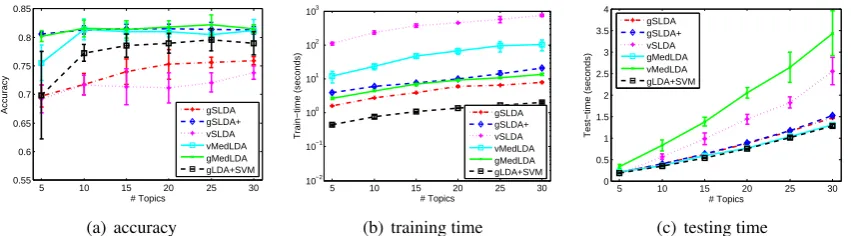
[image:6.595.88.514.55.173.2](c) testing time Figure 1: Accuracy, training time (in log-scale) and testing time on the 20NG binary data set.
candM in a wide range.
Fig. 1 shows the performance of different meth-ods with various numbers of topics. For accuracy, we can draw two conclusions: 1) without making restricting assumptions on the posterior distribu-tions, gSLDA achieves higher accuracy than vSL-DA that uses strict variational mean-field approxi-mation; and 2) by using the regularization constant
cto improve the influence of supervision
informa-tion, gSLDA+ achieves much better classification results, in fact comparable with those of MedLDA models since they have the similar mechanism to improve the influence of supervision by tuning a regularization constant. The fact that gLDA+SVM performs better than the standard gSLDA is due to the same reason, since the SVM part of gL-DA+SVM can well capture the supervision infor-mation to learn a classifier for good prediction, while standard sLDA can’t well-balance the influ-ence of supervision. In contrast, the well-balanced gSLDA+ model successfully outperforms the two-stage approach, gLDA+SVM, by performing topic discovery and prediction jointly4.
For training time, both gSLDA and gSLDA+ are very efficient, e.g., about 2 orders of magnitudes faster than vSLDA and about 1 order of magnitude faster than vMedLDA. For testing time, gSLDA and gSLDA+ are comparable with gMedLDA and the unsupervised gLDA, but faster than the varia-tional vMedLDA and vSLDA, especially whenK
is large.
4.2 Multi-class classification
We perform multi-class classification on the 20NG data set with all the 20 categories. For multi-class multi-classification, one possible extension is to use a multinomial logistic regression model for categorical variables Y by using topic
represen-tations ¯z as input features. However, it is
non-4The variational sLDA with a well-tunedcis significantly
better than the standard sLDA, but a bit inferior to gSLDA+.
trivial to develop a Gibbs sampling algorithm us-ing the similar data augmentation idea, due to the presence of latent variables and the nonlinearity of the soft-max function. In fact, this is harder than the multinomial Bayesian logistic regression, which can be done via a coordinate strategy (Pol-son et al., 2012). Here, we apply the binary gSL-DA to do the multi-class classification, following the “one-vs-all” strategy, which has been shown effective (Rifkin and Klautau, 2004), to provide some preliminary analysis. Namely, we learn 20 binary gSLDA models and aggregate their predic-tions by taking the most likely ones as the final predictions. We again evaluate two versions of gSLDA – the standard gSLDA with c = 1 and the improved gSLDA+ with a well-tunedcvalue.
Since gSLDA is also insensitive toαandcfor the multi-class task, we setα = 5.6for both gSLDA and gSLDA+, and setc= 256for gSLDA+. The number of burn-in is set asM = 40, which is suf-ficiently large to get stable results, as we shall see. Fig. 2 shows the accuracy and training time. We can see that: 1) by using Gibbs sampling without restricting assumptions, gSLDA performs better than the variational vSLDA that uses strict mean-field approximation; 2) due to the imbalance be-tween the single supervision and a large set of word counts, gSLDA doesn’t outperform the de-coupled approach, gLDA+SVM; and 3) if we in-crease the value of the regularization constant c,
algorith-20 30 40 50 60 70 80 90 100 110 0.55
0.6 0.65 0.7 0.75 0.8
# Topics
Accuracy gSLDA
gSLDA+ vSLDA vMedLDA gMedLDA gLDA+SVM
(a) accuracy
20 30 40 50 60 70 80 90 100110 10−1
100
101
102
103
104
105
# Topics
Train−time (seconds)
gSLDA gSLDA+ vSLDA vMedLDA gMedLDA gLDA+SVM
parallel−gSLDA parallel−gSLDA+
[image:7.595.76.288.58.164.2](b) training time Figure 2: Multi-class classification. Table 1: Split of training time over various steps.
SAMPLEλ SAMPLEη SAMPLEZ
K=20 2841.67 (65.80%) 7.70 (0.18%) 1455.25 (34.02%) K=30 2417.95 (56.10%) 10.34 (0.24%) 1888.78 (43.66%) K=40 2393.77 (49.00%) 14.66 (0.30%) 2476.82 (50.70%) K=50 2161.09 (43.67%) 16.33 (0.33%) 2771.26 (56.00%)
m without factorization assumptions is the main factor for the improved performance.
For training time, gSLDA models are about 10 times faster than variational vSLDA. Table 1 shows in detail the percentages of the training time (see the numbers in brackets) spent at each pling step for gSLDA+. We can see that: 1) sam-pling the global variablesηis very efficient, while
sampling local variables(λ,Z)are much more ex-pensive; and 2) samplingλis relatively stable as
K increases, while sampling Z takes more time
asK becomes larger. But, the good news is that
our Gibbs sampling algorithm can be easily paral-lelized to speedup the sampling of local variables, following the similar architectures as in LDA.
A Parallel Implementation: GraphLab is a graph-based programming framework for parallel computing (Gonzalez et al., 2012). It provides a high-level abstraction of parallel tasks by express-ing data dependencies with a distributed graph. GraphLab implements a GAS (gather, apply, scat-ter) model, where the data required to compute a vertex (edge) are gathered along its neighboring components, and modification of a vertex (edge) will trigger its adjacent components to recompute their values. Since GAS has been successfully ap-plied to several machine learning algorithms5
in-cluding Gibbs sampling of LDA, we choose it as a preliminary attempt to parallelize our Gibbs sam-pling algorithm. A systematical investigation of the parallel computation with various architectures in interesting, but beyond the scope of this paper.
For our task, since there is no coupling among the 20 binary gSLDA classifiers, we can learn them in parallel. This suggests an efficient hybrid multi-core/multi-machine implementation, which
5http://docs.graphlab.org/toolkits.html
can avoid the time consumption of IPC (i.e., inter-process communication). Namely, we run our ex-periments on a cluster with 20 nodes where each n-ode is equipped with two 6-core CPUs (2.93GHz). Each node is responsible for learning one binary gSLDA classifier with a parallel implementation on its 12-cores. For each binary gSLDA mod-el, we construct a bipartite graph connecting train documents with corresponding terms. The graph works as follows: 1) the edges contain the to-ken counts and topic assignments; 2) the vertices contain individual topic counts and the augment-ed variables λ; 3) the global topic counts and η
are aggregated from the vertices periodically, and the topic assignments and λ are sampled
asyn-chronously during the GAS phases. Once start-ed, sampling and signaling will propagate over the graph. One thing to note is that since we can-not directly measure the number of iterations of an asynchronous model, here we estimate it with the total number of topic samplings, which is again aggregated periodically, divided by the number of tokens. We denote the parallel models by parallel-gSLDA (c = 1) and parallel-gSLDA+ (c = 256). From Fig. 2 (b), we can see that the parallel gSL-DA models are about 2 orders of magnitudes faster than their sequential counterpart models, which is very promising. Also, the prediction performance is not sacrificed as we shall see in Fig. 4.
4.3 Sensitivity analysis
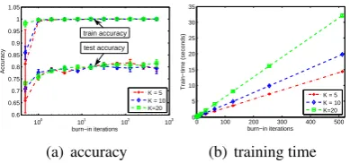
Burn-In: Fig. 3 shows the performance of gSL-DA+ with different burn-in steps for binary classi-fication. WhenM = 0(see the most left points), the models are built on random topic assignments. We can see that the classification performance in-creases fast and converges to the stable optimum with about 20 burn-in steps. The training time in-creases about linearly in general when using more burn-in steps. Moreover, the training time increas-es linearly asKincreases. In the previous
experi-ments, we setM = 100.
100 101 102 103 0.6 0.65 0.7 0.75 0.8 0.85 0.9 0.95 1 1.05 burn−in iterations Accuracy
K = 5 K = 10 K=20 train accuracy
test accuracy
(a) accuracy
0 100 200 300 400 500 0 5 10 15 20 25 30 35 burn−in iterations Train−time (seconds)
K = 5 K = 10 K=20
[image:8.595.85.280.58.149.2](b) training time Figure 3: Performance of gSLDA+ with different burn-in steps for binary classification. The most left points are for the settings with no burn in.
10−1 100 101 102 103 0.5 0.55 0.6 0.65 0.7 0.75 0.8 0.85 burn−in iterations Accuracy
K = 20 K = 30 K = 40 K = 50
gSLDA+ parallel−gSLDA+ (a) accuracy 10−1 100 101 102 103 100 101 102 103 104 105 burn−in iterations Train−time (sec)
K = 20 K = 30 K = 40 K = 50
parallel−gSLDA+ gSLDA+
[image:8.595.307.525.58.290.2](b) training time Figure 4: Performance of gSLDA+ and parallel-gSLDA+ with different burn-in steps for multi-class multi-classification. The most left points are for the settings with no burn in.
burn-in steps increases. Even when we use 40 or 60 burn-in steps, the training time is still compet-itive, compared with the variational vSLDA. For parallel-gSLDA+ using GraphLab, the training is consistently about 2 orders of magnitudes faster. Meanwhile, the classification performance is also comparable with that of gSLDA+, when the num-ber of burn-in steps is larger than 40. In the pre-vious experiments, we have setM = 40for both gSLDA+ and parallel-gSLDA+.
Regularization constant c: Fig. 5 shows the
performance of gSLDA in the binary classification task with differentcvalues. We can see that in a wide range, e.g., from 9 to 100, the performance is quite stable for all the threeK values. But for
the standard sLDA model, i.e., c = 1, both the training accuracy and test accuracy are low, which indicates that sLDA doesn’t fit the supervision da-ta well. Whenc becomes larger, the training ac-curacy gets higher, but it doesn’t seem to over-fit and the generalization performance is stable. In the above experiments, we setc= 25. For multi-class multi-classification, we have similar observations and setc= 256in the previous experiments.
Dirichlet prior α: Fig. 6 shows the
perfor-mance of gSLDA on the binary task with differ-entαvalues. We report two cases withc= 1and
c = 9. We can see that the performance is quite stable in a wide range ofα values, e.g., from0.1
1 2 3 4 6 7 8 9 10 0.65 0.7 0.75 0.8 0.85 0.9 0.95 1 1.05 √c Accuracy
K = 5 K = 10 K = 20
train accuracy test accuracy
(a) accuracy
1 2 3 4 6 7 8 9 10 1 2 3 4 5 6 7 8 9 10 11 √c Train−time (seconds)
K = 5 K = 10 K = 20
(b) training time Figure 5: Performance of gSLDA for binary clas-sification with differentcvalues.
10−4 10−2 100 102 104
0.5 0.55 0.6 0.65 0.7 0.75 0.8 0.85 α Accuracy
K = 5 K = 10 K = 15 K=20
(a)c= 1
10−6 10−4 10−2 100 102 104
0.55 0.6 0.65 0.7 0.75 0.8 0.85 α Accuracy
K = 5 K = 10 K = 15 K=20
(b)c= 9
Figure 6: Accuracy of gSLDA for binary classifi-cation with differentαvalues in two settings with c= 1andc= 9.
to10. We also noted that the change ofαdoes not
affect the training time much.
5 Conclusions and Discussions
We present two improvements to Bayesian logis-tic supervised topic models, namely, a general for-mulation by introducing a regularization parame-ter to avoid model imbalance and a highly efficient Gibbs sampling algorithm without restricting as-sumptions on the posterior distributions by explor-ing the idea of data augmentation. The algorithm can also be parallelized. Empirical results for both binary and multi-class classification demonstrate significant improvements over the existing logistic supervised topic models. Our preliminary results with GraphLab have shown promise on paralleliz-ing the Gibbs samplparalleliz-ing algorithm.
For future work, we plan to carry out more careful investigations, e.g., using various distribut-ed architectures (Ahmdistribut-ed et al., 2012; Newman et al., 2009; Smola and Narayanamurthy, 2010), to make the sampling algorithm highly scalable to deal with massive data corpora. Moreover, the data augmentation technique can be applied to deal with other types of response variables, such as count data with a negative-binomial likeli-hood (Polson et al., 2012).
Acknowledgments
[image:8.595.309.526.61.153.2] [image:8.595.77.288.204.300.2]2012CB316301), Tsinghua Initiative Scientific Research Program No.20121088071, Tsinghua National Laboratory for Information Science and Technology, and the 221 Basic Research Plan for Young Faculties at Tsinghua University.
References
A. Ahmed, M. Aly, J. Gonzalez, S. Narayanamurthy, and A. Smola. 2012. Scalable inference in laten-t variable models. InInternational Conference on Web Search and Data Mining (WSDM).
D.M. Blei and J.D. McAuliffe. 2010. Supervised topic models. arXiv:1003.0783v1.
D.M. Blei, A.Y. Ng, and M.I. Jordan. 2003. Latent Dirichlet allocation.JMLR, 3:993–1022.
M. Chen, J. Ibrahim, and C. Yiannoutsos. 1999. Pri-or elicitation, variable selection and Bayesian com-putation for logistic regression models. Journal of Royal Statistical Society, Ser. B, (61):223–242. P. Germain, A. Lacasse, F. Laviolette, and M.
Marc-hand. 2009. PAC-Bayesian learning of linear clas-sifiers. In International Conference on Machine Learning (ICML), pages 353–360.
A. Globerson, T. Koo, X. Carreras, and M. Collins. 2007. Exponentiated gradient algorithms for log-linear structured prediction. InICML, pages 305– 312.
J.E. Gonzalez, Y. Low, H. Gu, D. Bickson, and C. Guestrin. 2012. Powergraph: Distributed graph-parallel computation on natural graphs. Inthe 10th USENIX Symposium on Operating Systems Design and Implementation (OSDI).
T.L. Griffiths and M. Steyvers. 2004. Finding scientif-ic topscientif-ics. Proceedings of National Academy of Sci-ence (PNAS), pages 5228–5235.
Y. Halpern, S. Horng, L. Nathanson, N. Shapiro, and D. Sontag. 2012. A comparison of dimensionality reduction techniques for unstructured clinical text. InICML 2012 Workshop on Clinical Data Analysis. C. Holmes and L. Held. 2006. Bayesian auxiliary vari-able models for binary and multinomial regression. Bayesian Analysis, 1(1):145–168.
Q. Jiang, J. Zhu, M. Sun, and E.P. Xing. 2012. Monte Carlo methods for maximum margin supervised top-ic models. InAdvances in Neural Information Pro-cessing Systems (NIPS).
T. Joachims. 1999. Making large-scale SVM learning practical. MIT press.
S. Lacoste-Jullien, F. Sha, and M.I. Jordan. 2009. Dis-cLDA: Discriminative learning for dimensionality reduction and classification. Advances in Neural In-formation Processing Systems (NIPS), pages 897– 904.
Y. Lin. 2001. A note on margin-based loss functions in classification.Technical Report No. 1044. Universi-ty of Wisconsin.
D. McAllester. 2003. PAC-Bayesian stochastic model selection. Machine Learning, 51:5–21.
M. Meyer and P. Laud. 2002. Predictive variable selec-tion in generalized linear models. Journal of Ameri-can Statistical Association, 97(459):859–871.
D. Newman, A. Asuncion, P. Smyth, and M. Welling. 2009. Distributed algorithms for topic models. Journal of Machine Learning Research (JMLR), (10):1801–1828.
N.G. Polson, J.G. Scott, and J. Windle. 2012. Bayesian inference for logistic models using Polya-Gamma latent variables. arXiv:1205.0310v1.
R. Rifkin and A. Klautau. 2004. In defense of one-vs-all classification. Journal of Machine Learning Research (JMLR), (5):101–141.
L. Rosasco, E. De Vito, A. Caponnetto, M. Piana, and A. Verri. 2004. Are loss functions all the same? Neural Computation, (16):1063–1076.
A. Smola and S. Narayanamurthy. 2010. An architec-ture for parallel topic models. Very Large Data Base (VLDB), 3(1-2):703–710.
M.A. Tanner and W.-H. Wong. 1987. The calcu-lation of posterior distributions by data augmenta-tion. Journal of the Americal Statistical Association (JASA), 82(398):528–540.
D. van Dyk and X. Meng. 2001. The art of data aug-mentation. Journal of Computational and Graphi-cal Statistics (JCGS), 10(1):1–50.
C. Wang, D.M. Blei, and Li F.F. 2009. Simultaneous image classification and annotation. IEEE Confer-ence on Computer Vision and Pattern Recognition (CVPR).
J. Zhu, N. Chen, and E.P. Xing. 2011. Infinite latent SVM for classification and multi-task learning. In Advances in Neural Information Processing Systems (NIPS), pages 1620–1628.
J. Zhu, A. Ahmed, and E.P. Xing. 2012. MedLDA: maximum margin supervised topic models. Journal of Machine Learning Research (JMLR), (13):2237– 2278.
J. Zhu, N. Chen, H. Perkins, and B. Zhang. 2013a. Gibbs max-margin topic models with fast sampling algorithms. In International Conference on Ma-chine Learning (ICML).