Tool Wear Classification Using Fuzzy Logic for Machining
of Al/SiC Composite Material
V. Kalaichelvi1, R. Karthikeyan2, D. Sivakumar3, V. Srinivasan4 1Department of Electronics & Instrumentation Engineering, BITS-Pilani, Dubai Campus,
Dubai, United Arab Emirates
2Department of Mechanical Engineering, BITS-Pilani, Dubai Campus,
Dubai, United Arab Emirates
3Department of Electronics &Instrumentation Engineering, Annamalai University, Annamalai Nagar, India 4Department of Manufacturing Engineering, Annamalai University, Annamalai Nagar, India
Email: [email protected]
Received December 29,2011; revised February 7, 2012; accepted March 5, 2012
ABSTRACT
Tool wear state classification has good potential to play a critical role in ensuring the dimensional accuracy of the work piece and prevention of damage to cutting tool in machining process. During machining process, tool wear is an impor- tant factor which contributes to the variation of spindle motor current, speed, feed and depth of cut. In the present work, on-line tool wear state detecting method with spindle motor current in turning operation for Al/SiC composite material is presented. By analyzing the effects of tool wear as well as the cutting parameters on the current signal, the models on the relationship between the current signals and the cutting parameters are established with partial design taken from experimental data and regression analysis. The fuzzy classification method is used to classify the tool wear states so as to facilitate defective tool replacement at the proper time.
Keywords: Tool Wear Classification; Current Signal; Regression Analysis; Fuzzy Classification
1. Introduction
The development of an effective means to monitor the wear condition of cutting tools is one of the most impor- tant issues in the automation of the cutting process [1]. The consequences of non detection of tool failure may result in a poor quality of product and damage to the work piece or machine [2-4]. Many researchers have looked for ways to detect tool wear states. A large variety of sensors can be used for tool condition sensing. But only a few are reliable and effective. Direct measurement of tool wear using optical methods can be applied only when the tool is not in contact with the workpiece [5].
Indirect methods that rely on the relationship between tool states and measured signals to estimate the tool wear states have been extensively studied. Among the used sensors for monitoring tool condition, motor current sensing constitutes a major method (X. L. Li and S. K. Tso, [6] and Mannan et al., [7] described the feasibility of motor power and motor current sensing for adaptive control and tool condition monitoring. Mannan and Nilsson [8] presented a method using motor current measured from the spindle motor and feed motor to esti-mate the static torque and thrust in drilling and then to monitor the tool condition. The major advantage of using
the measurement of motor current to detect any malfunc-tion in the cutting process is that the measuring apparatus does not disturb the machining process. Moreover it can be applied in the manufacturing environment at almost no extra cost [9].
Most of the indirect approaches have been developed for fixed cutting conditions. In practical applications, however the cutting conditions are not fixed. The spindle speed and feed rate might change according to control strategies. Therefore wear estimation strategy that oper- ates under varying cutting conditions is much needed [10]. A successful monitoring system can effectively maintain machine tools, cutting tool and work piece. Re- search to date has shown that there are four parameters including cutting force, acoustic emission, motor current and vibration, which could be used to monitor tool, wear condition during turning operation.
variation in observed Y values can be contributed to this relation [11].
It is very important to develop a reliable and inexpen- sive intelligent monitoring system for use in cutting proc- esses. A successful monitoring system can effectively maintain machine tools, cutting tools and workpiece [12]. Artificial Neural Network (ANN) can approximate con- tinuous nonlinear functions well, and it is based on the mathematical principles and models of biological neu- rons and the nervous system. ANN has recently been applied to tool wear monitoring by some researchers. Q. Liu and Y. Altintas [13] have designed Multi-layer feed-forward neural network using force ratio, cutting speed and feed as input variables and flank wear as out-put response in turning operation. Y. X. Yao et al., [14] have proposed a new method for tool wear detection with different cutting conditions and detected signals which includes the model of wavelet fuzzy neural network with acoustic emission (AE) and the model of fuzzy classifi-cation with motor current.
In the present study, the current of the spindle motor is used to estimate the flank wear state. The current de- pends on the cutting parameters viz, the spindle speed (v), the feed rate (f), and depth of cut (d), as well as its wear (Vb). This paper implements a method for on-line estima- tion of flank wear from the currents measured using re- gression technology and a fuzzy classification method over a wide range of cutting conditions. The essence of the method is to establish a simple model relating the measured current value and the flank wear state under different cutting conditions. Based on the model, the tool wear states can then be estimated from the knowledge of the cutting parameters and the motor current signal. Ac- cording to the tool wear states obtained, the decision about tool replacement can be made.
2. Experimentation on Metal Cutting
Process
The essence of the method is to establish a simple model relating the measured current value and the flank wear state under different cutting conditions. Experiments are carried out in a Computer Numerical Control (CNC) lathe using K10 cemented carbide tool. The work piece material used for the experiment is LM25 Al (Alumin-
ium)/10% SiCp (Silicon Carbide) particulate reinforced
[image:2.595.352.496.330.440.2]composite material prepared through stir casting. The cutting conditions used for experimentation are listed in
Table 1.
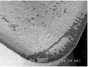
Cutting tests are performed on a (CNC) Lathe driven by Permanent Magnet Direct Current (PMDC) motor. A PMDC motor is similar to an ordinary DC shunt motor except that its field is provided by permanent magnet instead of salient pole wound field structure. In such motors torque is produced by interaction between the axial current carrying conductors and the magnetic flux produced by the permanent magnets. The DC motor cur- rent of the lathe is measured. A personal computer is interfaced with the turning lathe. The cutting conditions are provided as data to the computer and the cutting op- eration is performed automatically. Figure 1 to Figure 3
show the scanning electron microscopy images of worn out tool in different cutting conditions with varying in- tensity of wear.
[image:2.595.351.496.476.585.2]Figure 1. Wear at v = 250 rpm, f = 1.1 mm/rev and d = 0.8 mm.
[image:2.595.53.539.640.733.2]Figure 2. Wear at v = 740 rpm, f = 1.1 mm/rev and d = 0.8 mm.
Table 1. Experimental conditions for metal cutting process.
Spindle speed 250, 740 and 1150 rpm
Feed rates 0.05 and 1.07 mm/rev
Depth of cut 0.5, 0.75 and 1.0 mm Cutting conditions
Flank wear 0.3, 0.4, 0.5, 0.6, 0.7, 0.8 and 0.9 mm
Work piece Al +10% of SiC particulate reinforced composite material
Cutting tool K10 cemented carbide
Figure 3. Wear at v = 740 rpm, f = 1.1 mm/rev and d = 1 mm.
Experiments are conducted for various sets of cutting conditions that include spindle speed, feed rate and depth of cut. For each set of cutting conditions, machining is done starting with a fresh tool inserted continuing until the tool worn out A total of 56 tool wear cutting tests are conducted under different cutting conditions, 35 sample data are randomly selected and used as learning samples as shown in Table 2.
The remaining 21 samples are used as the test samples in the classification phase as illustrated in Table 3.
3. Prediction of Flank Wear Using
Regression Analysis and Fuzzy
Classification
Regression analysis is a statistical forecasting model that is concerned with describing and evaluating the relation- ship between a given variable usually called dependent variable and one or more other variables known as the independent variables. In the present work, a regression method is used to determine the model for the spindle motor current as a function of the spindle speed v (rpm), feed rate f (mm/rev) and depth of cut d (mm). The model was approximately modified so as to describe the flank wear states wisuch as 0.30, 0.40, 0.50, 0.60, 0.70, 0.80 and 0.90 (mm) for . For different values of cutting conditions the current values are noted experi- mentally and the corresponding wear values are noted at particular time intervals.
1, ,7 i
The effect of the cutting variables v, f, and d on the current signals, for a sharp tool can be represented by the following equation:
1 2 3
0
a a a
IK v f d (1) where I is the current and K0 depends on the tool geome-
try and work piece material. Taking the logarithmic value of I for differ rent tool wear values, the spindle motor current Si where denotes the respective wear values and are given by
1, ,7 i
1 01 11ln 21ln 31ln
S a a va f a d w1 = 0.3 mm (2)
2 02 12ln 22ln 32ln
S a a va f a d w2 = 0.4 mm (3)
Table 2. Experimental cutting conditions and current sig- nals.
Feed rate (mm/rev)
Depth of cut (mm)
Flank wear (mm)
Spindle motor current (mA)
0.05 0.75 0.3 892 1.07 0.75 0.3 956 1.07 0.5 0.3 968
1.07 0.75 0.3 1094 1.07 1 0.3 1126 0.05 0.75 0.4 934 1.07 0.75 0.4 982
1.07 0.5 0.4 986 1.07 0.75 0.4 1173 1.07 1 0.4 1227
0.05 0.75 0.5 968 1.07 0.75 0.5 1004 1.07 0.5 0.5 1027
1.07 0.75 0.5 1228 1.07 1 0.5 1255 0.05 0.75 0.6 985 1.07 0.75 0.6 1027
1.07 0.5 0.6 1042 1.07 0.75 0.6 1249 1.07 1 0.6 1284
0.05 0.75 0.7 1007 1.07 0.75 0.7 1045 1.07 0.5 0.7 1085
1.07 0.75 0.7 1293 1.07 1 0.7 1304 0.05 0.75 0.8 1021 1.07 0.75 0.8 1068
1.07 0.5 0.8 1104 1.07 0.75 0.8 1312 1.07 1 0.8 1338
0.05 0.75 0.9 1058 1.07 0.75 0.9 1116 1.07 0.5 0.9 1163 1.07 0.75 0.9 1372
1.07 1 0.9 1415
3 03 13ln 23ln 33ln
S a a va f a d w3= 0.5 mm (4)
4 04 14ln 24ln 34ln
S a a va f a d w4 = 0.6 mm (5)
5 05 15ln 25ln 35ln
S a a va f a d w5 = 0.7 mm (6)
6 06 16ln 26ln 36ln
S a a va f a d w6 = 0.8 mm (7)
7 07 17ln 27ln 37ln
[image:3.595.301.538.121.689.2]Table 3. Experimental cutting conditions and current sig- nals for test cases.
Cutting speed (rpm)
Feed rate (mm/rev)
Depth of cut (mm)
Flank wear (mm)
Spindle motor current (mA)
1150 0.05 1 0.3 997
740 1.07 0.5 0.3 968
250 1.07 0.75 0.3 956
740 0.05 0.5 0.4 801
1150 1.07 0.75 0.4 1173
740 1.07 1 0.4 1227
250 0.05 0.75 0.5 814
740 1.07 0.5 0.5 1027
1150 0.05 1 0.5 1123
740 1.07 0.75 0.6 1189
740 0.05 0.5 0.6 846
1150 1.07 0.75 0.6 1249
250 1.07 1 0.7 1136
740 0.05 0.75 0.7 1007
1150 1.07 0.75 0.7 1293
740 0.05 0.75 0.8 1021
250 1.07 0.5 0.8 934
740 1.07 0.5 0.8 1104
1150 0.05 1 0.9 1232
740 1.07 0.5 0.9 1163
250 1.07 0.75 0.9 1116
The actual models derived from the experimental data become
1
2 1
511.1558 92.0064 ln 54.0223 ln 226.5482 ln 0.3 mm, 0.995
S v
d w R
f
f
f
f
f
f
f
(15)
where R2 is the correlation coefficient obtained in the regression analysis. It is observed that the cor
coefficients are very close to unity, and the relationship
with almost linear relationship.
Fi
(9)
2
2 2
357.9337 127.4543 ln 61.6012 ln 345.6559 ln 0.4 mm, 0.994
S v
d w R
(10)
3
2 3
287.3501 146.0524 ln 63.2407 ln 392.5424 ln 0.5 mm, 0.999
S v
d w R
(11)
4
2 4
321.3647 145.1459 ln 65.0159 ln 349.4221 ln 0.6 mm, 0.999
S v
d w R
(12)
5
2 5
243.7464 160.4426 ln 68.5357 ln 317.7824 ln 0.7 mm, 0.996
S v
d w R
(13)
6
2 6
278.1798 159.7316 ln 71.8728 ln 337.7303 ln 0.8 mm, 0.999
S v
d w R
(14)
7
2 7
274.2301 170.8532 ln 80.5139 ln 360.8119 ln 0.9 mm, 0.993
S v
d w R
relation
between the current signals and the cutting parameters is reasonably well represented by the proposed models for different tool wear states.
Figure 4 shows the effect of depth of cut on the cur-
rent signals. It is found that current signal increases as the depth of cut increases,
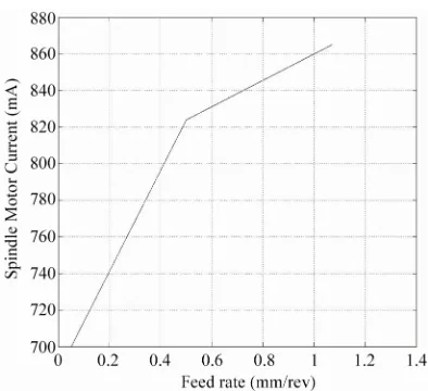
gure 5 shows the effect of the feed rate on the current
signal. Current signal increases as the feed rate increases. The reason for the condition is complex and is discussed by Shaw [15]. Figure 6 shows the main effect of the
spindle speed on the current signal. It is found that cur- rent signals increases with quadratic relation as the speed in increases. Figure 7 shows the effect of tool wear on
the current signals. Spindle motor current increases ex-
[image:4.595.323.522.307.511.2]Figure 4. Effect of depth of cut on current signal.
[image:4.595.324.521.536.716.2]Figure 6. Effect of spindle speed on current signal.
Figure 7. Effect of wear on current signal.
ponentially as tool wear increase with an almost incre- mental relationship. It is found that the tool wear has more significant effect on the spindle motor current. Based on above studies, it is seen that the tool wear, spindle speed, feed rate, dept of cut and current signals are related. The spindle motor current can be selected as a function of wear states in turning, taking into account the cutting parameters.
It has been recognized widely that the tool life can be divided into three phases characterized by three different wear processes, 1) break in, 2) normal wear and 3) ab- normal or catastrophic wear. The sudden rise in the wear rate observed during the abnormal tool wear phase is of interest here as an indication of the need for tool
placeme ear, the
tool wear curve usually fluctuates and is not smooth. The
the tool wear state as in Table 3. T
re-nt. Because many factors affect tool w
current signal models for the different wear states (flank wear = 0.3 0.9 mm) are established. The models can then be used to estimate the tool wear state from meas- ured current signals, and other cutting parameters. Thirty- five experimental results were used for the development of regression models (Table 2). Twenty-one additional
tests were conducted to examine the feasibility of using these models to estimate
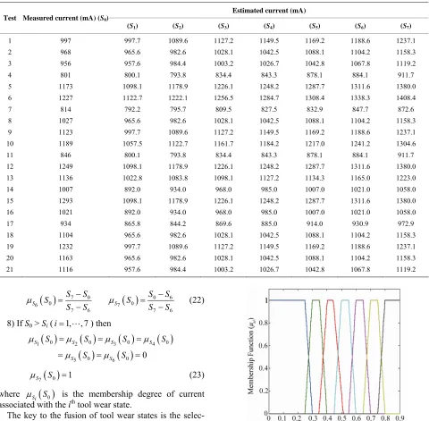
able 4 shows the comparison of the measured and es-
timated spindle current using Equations (9)-(15) respec- tively.
The measured current and estimated currents are de- fined as real feature values (S0) and estimated feature
values (Si) (where i1, ,7 ), respectively. S0 values
are compared in turn with the estimated feature values for different wear states ( 0.3 0.9 mm) in order to evaluate the degree of similarity between the real wear state to a estimated wear state.
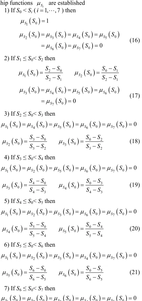
For the spindle motor current, the following member- ship functions Si
ny of the
are established 1) If S0 < Si (i1, ,7 ) then
01 1
S S
0 0 0 5 0
2 3 4
0 7 0
6
0
S S S S
S S
S S S S
S S
(16)
S
2) If 1≤ S0< S2 then
2 0 01
2 1
S
S S
S S
S
0 1
0 2
2 1
S
S S
S
S S
0 0 0
3 4 6
0 7
0
S S S
S
S S S
S
(17)
0 5
S S
3) If S2≤ S0< S3 then
0
0 5
0 6
S0 S7
S0 01 4
S S S S S S S
3 0 02
3 2
S
S S
S
S S
0 2
0 3
3 2
S
S S
S
S S
(18)
4) If S3≤ S0< S4 then
0
0 5
0
0 7
01 2 6 0
S S S S S S S S S S
4 0 03
4 3
S
S S
S
S S
0 30
4
4 3
S
S S
S
S S
(19)
5) If S4≤ S0< S5 then
0
0
0
0 7
0 01 2 3 6
S S S S S S S S S S
5 0 04
5 4
S S
S S
S S
0 4 05
5 4
S
S S
S
S S
(20)
6) If S5≤ S0< S6 then
0
0
0
0
01 2 3 4 0
S S S S S S S S
S S7
6 0 05
6 5
S S
S S
S S
0 5 06
6 5
S
S S
S
S S
(21)
7) If S6≤ S0< S7 then
0
0
0
0 5
01 2 3 4 0
S S S S S S S S S S
[image:5.595.66.283.284.436.2]Table 4. Compari nd estimated spindle motor current.
Estimated current (m
son of measured a
A)
T ) (S0)
(S1) (S2) (S3) (S4) (S5) (S6) ( 7
est Measured current (mA
S) 1 2 3 4 6 7 9 997 968 956 801 1227 814 1123 997.7 965.6 957.6 800.1 1098.1 792.2 965.6 1089.6 982.6 793.8 1178.9 795.7 982.6 1 1127. 1028.1 1003.2 834.4 1226.1 809.5 1028.1 1 1042.5 1026.7 843.3 1248.2 1 9.2 1088.1 1042.8 878.1 1287.7 9 1 1 1188.6 1104.2 1067.8 884.1 1311.6 1338.3 847.7 1104.2 1 1237.1 1158.3 1119.2 911.7 1380.0 1408.4 872.6 1158.3 1 2 1149.5 116
984.4
5 1173
1122.7 1222.1 1256.5 1284.7 1308.4
127.2 1161.7 834.4 1226.1 1098.1 968.0 1226.1 968.0 869.6 1028.1 1127.2 1028.1 1003.2 827.5 1042.5 832. 1088. 149.5 1184.2 843.3 1248.2 1127.2 985.0 1248.2 985.0 885.0 1042.5 1149.5 1042.5 1026.7 169.2 1217.0 878.1 1287.7 1134.3 1007.0 1287.7 1007.0 914.0 1088.1 1169.2 1088.1 1042.8 188.6 1241.2 884.1 1311.6 1165.0 1021.0 1311.6 1021.0 930.9 1104.2 1188.6 1104.2 1067.8 237.1 1304.6 911.7 1380.0 1223.0 1058.0 1380.0 1058.0 972.9 1158.3 1237.1 1158.3 1119.2 8 10 11 12 13 14 15 16 17 18 19 20 21 1027 1189 846 1249 1136 1007 1293 1021 934 1104 1232 1163 1116 089.6 1122.7 793.8 1178.9 1083.8 934.0 1178.9 934.0 844.2 982.6 1089.6 982.6 984.4 997.7 1057.5 800.1 1098.1 1022.8 892.0 1098.1 892.0 865.8 965.6 997.7 965.6 957.6
S7 0 0 6 6 S S S S 7 S
0 60 S 7 7 S S S S S 22)
f S0 > Si ) then
0
S
23) where is the membership degree of current
the ith tool state.
The key to the fusion of tool wear states is the selec- tio ate shape zy membership function for process variables based on experimental results. Fig- ure 8 shows the trapezoidal membership function of tool
wear states. The reason for choosing trapezoidal shape for tool wear states is that it is difficult to quantify an exact wear value.
g a wide
6
(
8) I (i1,,7
0 0
1 2 3 4
0 6 0
0
S S S S
S
S S S
S S
0
5 S
0 7S S
1 (
0Si S
associated with wear
n of appropri s of fuz
Figure 8. Fuzzy memberships of tool wear state.
where
w is the fuzzy membership value for tool wear states, and a, b, k and l are constants for different fuzzy sets. The constants ofwear conditions under the A, B, C, D, E, F and G classi- fication are shown in Table 5.
The outputs of the inference are still fuzzy values and they need to be defuzzified. Basically defuzzification is a mapping from a space of fuzzy values into that of the non-fuzzy universe. At present there are several strate- gies that can be used to perform the defuzzification proc-
fuzzy membership of tool Usin r range avoids defining an exact wear
value for a certain level of linguistic variable of tool wear. This will also allow an easy knowledge acquisition when developing a set of fuzzy rules for fuzzy inference. Based on the classification of tool wear states, the trapezoidal function is defined as follows [16].
w aw bTable 5. Constants of fuzzy membership functions for tool wear condition.
Constants of fuzzy functions for tool wear condition Tool wear
classification a B K l
A –20 0 1 6 0.25 0 0.25 0.3
B 20 0 –20 –5 1 8 0.25 0.3 0.35 0.3 0.35 0.4 C 20 0 –20 –7 1 10 0.35 0.4 0.45 0.4 0.45 0.5 D
20 –9 0.45 5
0.75 0.8 0 –20 1 12 0.5 0.55 0.55 0.6 0.
E 20 0 –20 –11 1 14 0.55 0.6 0.65 0.6 0.65 0.7
F 20 0 –20
–13 1 16
0.65
0.7 0.75 0.7
G 20 0 –15 1 0.75 0.8 0.8 0.9
ess. The most commonly used method is centroid method of defuzzification which produces the center of area of
the possibility distribution of inference output.
Therefore the defuzzified tool wear states can be ob- tained by using the formula
d Wear d w ww w w
w w
(25)where wear represents the numerical value of tool wear states and fuzzy membership degree fused by fuzzy in- ference.
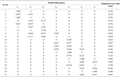
The membership degree of tool wear state with spindle current Si(w) where iA, B G is calculated using fuzzy classification method. The membership degrees of tool wear states are shown in Table 6.
4. Results and Discussion
A total of 55 tool wear cutting tests were conducted un- der various cutting conditions. 35 samples were randomly picked as learning samples and 21 samples were used as the test samples in the classification phase. The above method is used to estimate the tool wear value. The membership degrees of present tool states under different tool wear classification are calculated which is used by fuzzy inference.
Based on studies, it is suggested that the effects of tool Table 6. Membership degrees of tool wear states (test cases).
p degree Membershi Sl. No. 1 S
Estimated wear value (mm)
2 S
S3 S4 S5 S6 S7
1 2 4 5 7 8 10 12 13 15 16 17 18 21 0. 1. 0 0 0 0 27 24 11 0 0 0 0 0 142 0 0 0 0 0 0 0 0 0 0 0 0 0 0 0 0 0.250 0 0 853 0.922 0.979 0 0 0 0 0 0 0 0 0 0 0 0 0 0 0.146 0.077 0.020 0.944 1.000 0.778 0 0 0.0124 0 0 0 0 0 0 0 0 0 0 0 0 0 0 0.055 0 0.221 1.000 0.926 0.987 0.105 0 0 0 0 0 0 0 0 0 0 0 0 0 0 0 0 0 0.073 0 0.894 1.000 0.937 0.300 0.314 0.300 0.417 0.392 0.414 0.525 0.497 0.488 0.614 0.607 0.602 0.705 0.700 0.722 0.800 0.807 0.798 0.889 0.900 0.893 3 6 9 11 14 19 20 0 0 0 0 0 0 0 0 1.000 858 00 0 .073 0 0 0 0 0 0 0 0 0 0 0 0 0 0.141 0 0.822 0.9 0.857 0 0.0 0.1 0 0 0 0 0 0 0 0
0 0 0 0 0.062
[image:7.595.58.539.423.733.2]Table 7. C wear in turning.
B C D E F
lassification of tool
Classification A G
Tool wear value (mm) 0 - 0.3 0.25 - 0.4 0.35 - 0.5 0.45 - 0.6 0.55 - 0.7 0.65 - 0.8 0.75 - 0.9
wear indle sp eed rate and depth of t should taken o accou n modeling current In th prese work, th wear v re divi nto A, B C, D, E, F & G ificatio hown i ble 7. O
of th ain objectives of de g the t ar state to ob in a basis for replacing tools. D practical application a noticeable cha of the tool wear st has b n examined. Accordi he est tool wear state decision n be made if the tool should be r placed. The above method gi the tool ar state cording to previo ly collecte ata and t results. turni operation onitoring n be con cted by culating the mem rship grad f the curre servatio The replacem made when the grade wear in the curre observation exceeds a rtain thres old a .9. For th resent study, the rule for replaceme is suggested as follows:
“If the grade of membershi Si for the indle mot current is greater than 0.9 m then repl e the tool
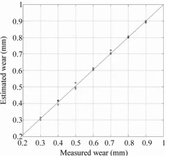
Figure shows the comparison between measured and
predicted values o ool wear
5. Conclusion
T we cutti ete
indle motor is analyzed. The model which shows the , sp eed, f
nt whe
cu be
in t signals.
d i
e nt e tool
class
alues a n as s
de
T
, ne n a
ool we
e m tectin is
ta uring
nges ates
ee ng to t imated
, a ca e-
ves we ac-
us d d est For
ng , m ca du cal-
be e o nt ob n.
tool ent decision is of
nt ce h-
s 0 e p nt
p sp or
m ac ”.
9
f T .
he effects of tool ar and ng param rs on the sp
[image:8.595.88.261.548.708.2]relationship between the current signals and cutting pa- rameters for different tool wear states (0.3 to 0.9) are established through experimental study and regression analysis. The membership function concept has been successfully used to calculate the grade of membership for given wear states and applied to the monitoring of tool wear state. The grade of membership associated with
Figure 9. Comparis ues of tool wear using fu
on between measured and predicted val- zzy classification method.
the relevant flank ear is always very clo nity based the established models. This indicates that the method is acceptable. The cont of tool re ent requires the recognition of the tool wear state associated with the cutting parameter including spindle speed and feed rate, which y change according to ontrol strategies. The use of the grades of member or the tool wear state pro des a scie basis for olling the t eplacem he me d is applic o the choi desi hreshold f wear acco the quality standard adopted.
FERENCES
[1] X i, S. Do P. K. Venuvinod, “Hyb arning
for Tool Wear rnational Jo of Ad-
vanced Manu ing Tec y, Vol. 16, 2000, 3-307. .1007/s00 00050161
w se to u
on
rol placem
ma the c
ship f vi ntific contr ool r ent. T tho able t ce of any red t o rding to
RE
. L ng and rid Le
urnal Monitoring,”
factur
Inte
hnolog No. 5,
pp. 30 doi:10 17
[2] L. C. Lee, K e and C an, “On the Correlation
between Dyna tting Tool Inter-
national Journal of Machin s and Manufacture, Vol. . S. Le . S. G
mic Cu Force and Wear,” e Tool
. 29, No. 3, 1989, pp. 295-303 doi:10.1016/0890-6955(89)90001-1
[3 S. B. Rao, “ al Cutting Machine Tool Design—A Re- w,” Jo anufactu ce and -
Tran f ASME, No. 4 .
713-716. doi:10.1115/1.2836814
] Met
vie ing
urnal of M sactions o
ring Scien Vol. 119,
Engineer , 1997, pp
[4] K. Danai and A. G. Ulsoy, “Dynamic State Model for On-Line Tool Wear Estimation in Turning,” Journal of Engineering for Industry, Transactions of ASME, Vol. 109, No. 4, 1987, pp. 396-399. doi:10.1115/1.3187145 [5] L. Dan and J. Mathew, “Tool Wear and Failure Monitor-
ing Techniques for Turning—A Review,” International Journal of Machine Tools and Manufacture, Vol. 30, No. 4, 1990, pp. 579-598. doi:10.1016/0890-6955(90)90009-8 [6] X. L. Li and S. K. Tso, “Drill Wear Monitoring Based on
Current Signals,” Wear, Vol. 231, No. 2, 1999, pp. 172- 178. doi:10.1016/S0043-1648(99)00130-1
[7] M. A. Mannan, S. Broms and B. Lindstrom, “Monitoring and Adaptive Control of Cutting Process by Means of Motor Power and Current Measurements,” CIRP An- nals—Manufacturing Technology, Vol. 38, No. 1, 1989, pp. 347-350. doi:10.1016/S0007-8506(07)62720-6 [8] M. A. Mannan and T. Nilsson, “The Behavior of Static
Torque and Thrust Due to Tool Wear in Drilling,” Tech-nical Papers of the North American Manufacturing Re-search Institution of ASME, 1997, pp. 75-80.
[10] Y. Koren, T. Ko and A. G. Ulsoy, “Flank Wear Estima- tion under Varying Cutting Conditions,” Journal of Dy- namic Systems, Measurement and Control, Vol. 113, No. 2, 1991, pp. 300-307.
[11] J. L. Devore and N. R. Farnum, “Applied Statistics for Engineers and Scientists,” 2nd Edition, Duxbury Press, Belmont, 2004.
[12] J. S. R. Jang, “Adaptive Network Based Fuzzy Inference Systems,” IEEE Transactions on Systems, Man and Cy- bernetics, Vol. 23, No. 3, 1999, pp. 665-685.
[13] Q. Liu and Y. Altintas, “On-Line Monitoring of Flank Wear in Turning with Multilayered Feed-Forward Neural Network,” International Journal of Machine Tools and
Manufacture, Vol. 39, No. 12, 1999, pp. 1945-1959.
doi:10.1016/S0890-6955(99)00020-6
[14] Y. X. Yao, X. L. Li and Z. J. Yuan, “Tool Wear Detection with Fuzzy Classification and Wavelet Fuzzy Neural Network,” International Journal of Machine Tools and Manufacture,Vol. 39, No. 10, 1999, pp. 1525-1538.
doi:10.1016/S0890-6955(99)00018-8
[15] M. C. Shaw, “Metal Cutting Principles,” Clarendon Press, Oxford, 1984.