Generalized additive models as an alternative approach to the modelling of the tree height diameter relationship

(1)

JOURNAL OF FOREST SCIENCE, 61, 2015 (6): 235–243

doi: 10.17221/14/2015-JFS

Generalized additive models as an alternative approach

to the modelling of the tree height-diameter relationship

Z. Adamec, K. Drápela

Department of Forest Management and Applied Geoinformatics, Faculty of Forestry and Wood Technology, Mendel University in Brno, Brno, Czech Republic

ABSTRACT: Generalized additive models were tested using three types of smoothing functions as an alternative for modelling the height curve. The models were produced for 23 forest stands of Norway spruce (Picea abies [L.] Karst.) in the territory of the Training Forest Enterprise Masaryk Forest Křtiny. The results show that the best evaluated and recommended for practical use at the level of forest stand was the LOESS function (locally weighted scatterplot smooting) when using a greater width of the bandwidth. Due to the frequent overfitting and the associated unrealistic behaviour of the function, smoothing by spline functions cannot be recommended for modelling the height curve at the level of forest stand. It was validated that the resulting model must be assessed not only according to the calcu-lated quality criteria, but also depending on the graphic pattern of the model which must ensure that the height curve pattern is realistic. The quality of the resulting models (with LOESS function) was assessed to be high, mainly due to the very precise determination of model heights.

Keywords: LOESS; nonparametric method; Norway spruce; Petterson function; smoothing function; spline

A large number of variables are measured as part of the forest inventory. Of these, tree height and di-ameter at breast height are considered to be essen-tial. Unlike measuring a diameter at breast height, which is easy and inexpensive, measuring height consumes considerable time and money (Adame et al. 2008). Although the cost of the latter can be reduced due to the use of distance-measuring ultrasound and laser technology, height measure-ment is still a very labour-intense method (Var-gas-Larreta et al. 2009). Therefore fitted heights are often used instead of measured heights. Fitted heights are derived from the model of the height-diameter relationship which is compiled from the measured heights and diameters (Huang et al.

1992; Martin, Flewelling 1998). A height curve is graphical expression of the height-diameter re-lationship. According to Schmidt et al. (2011), attempts to reduce costs of height measurement made the height-diameter relationship model one of the most important results of the evaluation of forest inventory data.

The height curve model is one of the regression models and can be written down using a

math-ematical relationship referred to as the height function and designed especially for this purpose. There is currently a large number of such func-tions; a comprehensive listing can be found e.g. in the papers of Peng (1999), Huang et al. (2000), Husch et al. (2003), Šmelko (2007) or Van Laar

and Akça (2007). Mehtätalo (2004) compared

(2)

placed on the least squares method (e.g. normal-ity and independence of residuals etc.) may often be a problem. Possible solutions to the problems outlined above include the use of nonparametric methods that are robust towards the conditions re-quired by the least squares method. Of these, a gen-eralized additive model (GAM) can be considered as an alternative for modelling the height-diameter relationship, a technique that employs different smooth functions to produce the model. The sum of smooth functions of covariates is included in the predictor of a GAM. Dependence of the response variable on the covariates in the GAM is speci-fied only in terms of smooth functions rather than detailed parametric relationships (Wood 2006). Writing down the equation with parameters is thus not possible. However, it is data that determines the resulting shape of the model. The final GAM therefore has a degree of flexibility that cannot be achieved in linear or nonlinear modelling (Rob-inson et al. 2011). The same authors referred to GAMs as being suitable for modelling in forestry at the very moment when the task is the best pos-sible fitting rather than making the best estimate of model parameters. Wang et al. (2005) reported that GAMs are more resistant to extreme values than other linear or nonparametric methods. The same conclusions were reached by Byun et al. (2013) in their paper. Moisen et al. (2006) pointed to the fact that in addition to fitting quality, GAMs are easy to interpret. In forestry, this modelling technique can be encountered in a range of applications over the past few years, e.g. in the papers of Falk and Mel-lert (2011) and Kouba and Alados (2012), who dealt with the modelling of spatial dynamics of tree species, Wang et al. (2005), AlbertandSchmidt (2010) and Aertsen et al. (2012), who discussed the site-specific production capacity, Robinson et al. (2011) and Kuželka and Marušák (2014), who modelled the stem form or Byun et al. (2013), who modelled the diameter growth of trees or Zhang et al. (2008) and Schmidt et al. (2011), who modelled exactly height curves of various tree species, but used only different spline functions without using the LOESS function. Based on previous statements, three key advantages suggest to prefer a GAM in-stead of a classic height curve: (i) higher flexibility of the model, (ii) robustness against outliers, (iii) no usage limitations as in the case of OLS regres-sion (normality or independence of residuals).

All three advantages overlap, which implies that GAM-based height curve could be utilized in forest stands where OLS-based methods do not perform satisfactorily or where preconditions for OLS

ap-plication are not met. A typical example is a for-est stand with higher diameter or height variability where a few suppressed or, on the contrary, domi-nating trees can affect the height curve position and thus the resulting model.

The aim of this study is to assess the possibility of practical use of various types of generalized addi-tive models as alternaaddi-tives for modelling the height curve on the level of forest stand with special em-phasis being placed on the resulting quality of the fitted model.

MATERIAL AND METHODS

Data were collected in the territory of Masaryk Forest Křtiny Training Forest Enterprise, the spe-cial-purpose premises of Mendel University in Brno. It involved 23 forest stands of Norway spruce (Picea abies [L.] Karst.), the age range being 30 to 136 years. Two sample plots were placed in each for-est stand. The plot size was determined based on the requirement for a sufficient number of trees per plot and graded per age. The size of the plots was 250 m2 (r = 8.92 m) in stands under 40 years, 700 m2 _in stands aged 41–80 years (r = 14.93 m), and 1,200 m2 in stands aged 81 years and more (r = 19.54 m). Tree height using a Vertex Laser hypsometer to the near-est 0.1 m and diameter at breast height using a calli-per to the nearest 1 cm were measured on the plots. A total of 1,590 trees were measured.

GAMs were compiled for three different smooth-ing functions: these involved spline, cubic spline and LOESS types. A GAM can be written down us-ing the Equation (1):

∧

h_i = a + f_s (d_1.3_i) + ε_i (1)

where: ∧

h_i – fitted height of a tree i,

a – intercept of the model,

f_s – smoothing function,

d_1.3_i – diameter at breast height of a tree i, ε_i – residual value.

(3)

resulting model becoming adjusted to the measured values too much regardless of the model’s practical applicability and sense. Subsequently, such a model cannot be applied to any other data, or at least its use gives very poor results.

Different methods are used for determining the op-timal degree of smoothing; this varies based on the type of smoothing function applied. In the event of the LOESS function, it is important to find the op-timal width, i.e. bandwidth; indicating the degree of smoothing, it specifies the width of the interval around each of the measured values. This whole in-terval is fitted with a function using linear-weighted regression and a fitted value is determined for the measured value (Zuur et al. 2009). A suitable band-width is searched for using the Akaike information criterion – AIC (Akaike 1973). In spline functions, the procedure is different. The data file is divided into segments separated by nodes. Individual segments are fitted by regression models (the spline function uses a linear model, while cubic spline uses the 3rd_degree polynomials). Segments are joined together where they form nodes. For more details about joining the segments refer to the paper of Wood (2006). The de-gree of smoothing is specified through the number of nodes. The optimal number of nodes is chosen using a leave-one-out cross-validation.

The models formed were compared with each other as well as with a traditional height curve computed by nonlinear regression using the Pet-terson function (PetPet-terson 1955). This function can be written down using the Equation (2):

∧

h_i= 1.3 + 1/(a + b/d_1.3_i)3 ₍₂₎

where: ∧

h_i – fitted height of a tree i,

a – intercept of the model,

b – regression parameter,

d_1.3_i – diameter at breast height of a tree i.

This function was chosen because it is recom-mended as a very good function in papers such as

Kramer and Akça (1995), Van Laar and Akça

(2007), Pretzsch (2009) or Drápela (2011). The mutual comparison of different models took place in each of the 23 forest stands separately. To compare different models, the following criteria were chosen: – Amount of explained deviance (Dobson 2002) (Eq. 3):

pseudo R2_{= 100}_×₍_D

0 – Dr)/D0 (3)

where:

D₀ – null deviance;

D_r – residual deviance.

– Akaike information criterion (Eq. 4): AIC = n × ln((∑e2

i)/n) + 2 × m (4)

where:

e_i – residual value,

n – sample size,

m – number of parameters. – Mean of residuals (Eq. 5):

ē_i= (∑e_i)/n (5)

where:

n – sample size,

e_i – residual value.

– Residual standard deviation (Eq. 6):

σ_ei=√(∑(e_i – ē_i)2_/n ₍₆₎

where:

n – sample size,

e_i – residual value,

ē_i – mean of residuals.

– Mean of deviation of fitted values obtained from the additive model and fitted values obtained from the nonlinear regression model (Eq. 7):

∆_ig= ∑n_i₌₁|^y_igam_–∧y_inlr|/n (8) where:

∧

y_igam – fitted value of a tree i (i = 1, 2, 3, …, n) from the additive model,

∧_y

inlr – fitted value of a tree i (i = 1, 2, 3, …, n) from the

non-linear regression model and n is the sample size. – Visual similarity to the height curve model fitted

by nonlinear regression,

– The realism of the model behaviour.

The realism of model behaviour implies that the model meets the general height curve requirements (Šmelko 2007). The most important is that the curve must be non-decreasing.

Deviance is calculated in models which use the maximum likelihood method (Zuur et al. 2009). Zero deviance equals the total sum of squares, while residual deviance corresponds to the residual sum of squares in regression models.

All calculations were performed using the R soft-ware (R Development Core Team 2013). The results are presented with 95% confidence, i.e. at the signifi-cance level of α = 0.05.

RESULTS

(4)

[image:4.595.62.526.72.753.2]

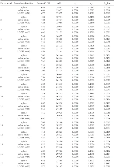
Table 1. Criteria for generalized additive models

Forest stand Smoothing function Pseudo R2_(%) _AIC –_e

i σei Δig (m)

1 cubic splinespline 68.668.6 194.97194.95 0.00000.0000 1.08871.0885 0.00680.0068

LOESS (0.70) 67.9 195.97 0.0000 1.1001 0.0063

LOESS (0.75) 42.8 139.68 0.0000 1.2140 0.0011

LOESS (0.65) 84.9 151.55 0.0000 0.9582 0.0023

LOESS (0.75) 74.3 160.77 0.0000 1.0010 0.0040

LOESS (0.60) 85.9 232.61 0.0000 0.9319 0.0050

LOESS (0.85) 76.4 263.63 0.0000 1.3409 0.0122

LOESS (0.80) 70.0 377.74 0.0000 1.4145 0.0054

LOESS (0.95) 74.7 261.98 0.0000 1.3893 0.0075

LOESS (0.85) 62.5 213.48 0.0000 1.4791 0.0041

LOESS (0.85) 72.7 366.51 0.0000 1.9564 0.0124

LOESS (0.80) 86.7 275.69 0.0000 1.3545 0.0059

LOESS (0.80) 69.2 271.23 0.0000 1.5483 0.0046

LOESS (0.85) 72.7 184.29 0.0000 1.2912 0.0034

LOESS (0.95) 42.1 288.64 0.0000 1.9891 0.0150

LOESS (0.75) 81.7 299.40 0.0000 1.5289 0.0056

LOESS (0.80) 58.8 300.29 0.0000 2.4693 0.0091

(5)

numerical results all functions used are acceptable and not a single type of smoothing function can be referred to as the best. However, in the graphics rendered by the used functions, the differences are already clearly visible. The spline functions have problems with overfitting, which caused in some cases a biologically unacceptable and unfounded shape of the function. For instance, there are sever-al cases of the height decreasing as the diameter in-creases. This is due to the choice of the method for finding an optimal degree of smoothing when the cross-validation actually seeks for a model that best fits the data field regardless of the practical use of the resulting model. Of the 23 forest stands, there was a problem with the realism of the behaviour in 5 cases for spline and in 8 cases for cubic spline. It is important to note that all the numerical results (shown in Table 1) in these forest stands showed no problems; indeed, they indicated a model of very good quality.

The LOESS function very well modelled the height-diameter relationship in all stands with a very similar behaviour of the function as a model of the Petterson height curve. It is due to this fact that the resulting model was chosen as a compro-mise between the degree of smoothing and the realism of its behaviour. Therefore the resulting model generated through the LOESS function may not have the best values of numerical criteria

com-pared with spline functions, but will always have a biological justification. The values of the resulting criteria were never so different from those obtained through spline functions to permit speaking of a model of lesser quality. Actually, the resulting mean values of deviations of the fitted values obtained through the additive model (using the LOESS func-tion) from the fitted values of nonlinear model (last column of Table 1) make it possible to refer to the resulting models as models with a very good capa-bility of fitting.

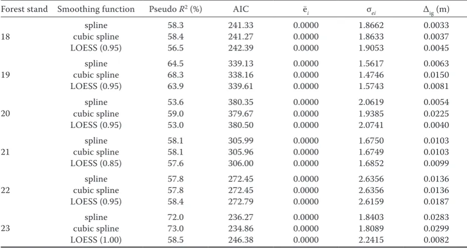
When the LOESS function was used, a model with the bandwidth exceeding 0.60 was selected to be the final model in all of the forest stands. It can therefore be concluded that rather a larger bandwidth should be chosen when using the LOESS function in GAMs at a local level to prevent the overfitting of the model. Graphical outputs of several forest stands are shown in Fig. 1. These three forest stands were se-lected to represent the whole set under study: the range of ages and other dendrometric variables such as heights and diameters. The ages of stands No. 3, 13 and 23 were 35, 88 and 136 years, respec-tively. Fig. 1a presents the behaviour of GAMs and that of the nonlinear model of the Petterson func-tion in forest stand No. 13; it is clearly shown that the models fitted using splines and cubic splines are practically unacceptable (the tree height decreas-ing as the diameter increases), while the behaviour Forest stand Smoothing function Pseudo R2_(%) _AIC –_e

i σei Δig (m)

LOESS (0.95) 56.5 242.39 0.0000 1.9053 0.0045

LOESS (0.95) 63.9 339.61 0.0000 1.5743 0.0081

LOESS (0.95) 53.0 380.50 0.0000 2.0741 0.0040

LOESS (0.85) 57.6 306.00 0.0000 1.6852 0.0099

LOESS (0.95) 58.4 272.79 0.0000 2.6159 0.0187

LOESS (1.00) 58.5 246.38 0.0000 2.2415 0.0082

pseudo R2_{(%) – amount of explained deviance, AIC – Akaike information criterion,}_e–

i– mean residual, σei – residual standard

[image:5.595.63.529.75.323.2]

deviation, Δ_ig – the mean of deviations of fitted values obtained from the additive model and fitted values obtained from the nonlinear regression model (with LOESS function a bandwidth is in the brackets)

(6)

the LOESS function shows is very similar to that of the Petterson model and the function has a realistic behaviour.

Fig. 1b also illustrates very well the overfitting of the model fitted through the spline functions in forest stand No. 23. The lack of realism of the model seen in this case is based on the fitted values oscillating around the nonlinear model of the Petterson func-tion. The model fitted through the LOESS function has a good and applicable behaviour again.

Fig. 1c shows the behaviour of GAMs and the non-linear model of the Petterson function in forest stand No. 3. With the behaviour of all the evaluated models being in fact consistent, the individual models overlap in the chart. All the models could be used to shape the height curve in the forest stand with no differences in the quality of fitting.

The generalized additive model using the LOESS function can be labelled a fully applicable and

suit-able alternative for modelling height curves using nonparametric methods. If this type is applied at the local level, i.e. a height curve model in the for-est stand, a larger bandwidth should be used to pre-vent overfitting and ensure the realistic behaviour of the modelled curve.

DISCUSSION

In the case of very complicated relationships be-tween the dependent and independent variables it is often very difficult to find a suitable mathemati-cal function for fitting the relationship (Robinson et al. 2011). Finding the right estimates of the pa-rameters of such a model is another common prob-lem. For modelling a height curve using GAMs, three different smoothing functions were tested ‒ spline, cubic spline and LOESS. They are recom-mended for use in forestry models e.g. by Moisen andFrescino (2002), Wang et al. (2005), Zhang et al. (2008), FalkandMellert (2011) and Yue et al. (2012).

For spline functions, cross-validation was chosen to be the method for selecting the optimum degree of smoothing. Even this method, however, failed in several cases to choose a model without overfitting.

Falk and Mellert (2011) denoted this method

to be very good while adding that monitoring the ecological understandability of the resulting model was still necessary.

The fact that, in all stands, the LOESS function performed better than the spline function can be attributed to the worse performance of spline func-tion when there was a higher data variability. This is apparent in Fig. 1. The previous statement implies that the use of GAM with LOESS function can be advantageous in stands with higher data variability.

According to the results obtained, GAMs can be considered a suitable alternative for modelling the height curve. The same conclusions were reported by Zhang et al. (2008) and Schmidt et al. (2011). Zhang et al. (2008) recommended this method as suitable for modelling the height curve after test-ing the GAM model ustest-ing the spline function on several tree species in Ontario, Canada. He also confirmed the hypothesis that the mean residuals of GAMs are lower than those of models calcu-lated by the least squares method. Schmidt et al. (2011) examined the compilation of a height curve in Scots pine (Pinus sylvestris L.) using the GAM model for the territory of Estonia with a penalised cubic spline used as the smoothing function. This function does not use different numbers of nodes; 26

28 30 32 34 36 38 40

20 30 40 50 60

22 24 26 28 30 32 34 36 38 40 42

20 24 28 32 36 40 44 48 52 56 60 64 68 72

H

ei

gh

t (

m

)

8 10 12 14 16 18 20 22 24

8 12 16 20 24 28 32 DBH (cm)

measured values

spline cubic spline

LOESS

[image:6.595.63.288.56.464.2]

Petterson function

Fig. 1. Fitted GAMs and non-linear regression model in forest stands No. 13 (a), No. 23 (b), and No. 3 (c)

(a)

(b)

(7)

instead, a large number of nodes are chosen and the degree of smoothing is determined by means of the parameter λ, the optimum value which is searched for applying cross-validation. Furthermore, this GAM model included also a stand variable; more specifically mean diameter at breast height of the stand, so that the author was able to produce a sys-tem of uniform height curves.

From a practical aspect, a height curve produced using GAM where the emphasis is placed on the most accurate determination of heights can be used. This means that it can find its application not only when identifying the standing volume using volume tables, but particularly also in modelling heights on research plots where the heights can be used for calculating the increment in height and subsequently in volume as part of repeated forest inventory operations. Modelling missing heights in stands that serve as a basis for growth simulation is another alternative. Using GAMs instead of ordi-nary parametric models thus eliminates the prob-lem of initial estimates of function parameters.

One of the results of our research was the state-ment that GAMs provided a very accurate fitting.

Zhang and Gove (2005) argued that in GAMs,

the good quality of fitting is due to their robustness and flexibility. Although they modelled the crown area – diameter at breast height relationship, their results can be regarded as a general statement for this method. Therefore it is possible to compare our results with those of ZhangandGove (2005).

It is stated in various papers that GAMs are capable of describing strongly nonlinear relation-ships occurring in an ecosystem (Byun et al. 2013) and also the behaviour of biological processes (Frescino et al. 2001; Austin 2002; Lehmann et al. 2003). This was only partially confirmed in our study because only the LOESS-based model was ecologically plausible and capable of modelling the nonlinear relationship of local scale height curve.

CONCLUSIONS

Based on the results obtained, GAMs can be considered as a suitable alternative for model-ling a height curve. Differences were shown be-tween smoothing functions when using them at the stand level. The LOESS type with a greater bandwidth can be described as the best as they prevented the overfitting of the resulting model. Overfitting was a problem for both the spline functions. The insufficient performance of spline functions could be caused by higher data

variabil-ity in forest stands under study. When selecting the resulting model, the decision cannot be driven solely by the calculated values of benchmarks; the graphical pattern of the model needs to be moni-tored with respect to the behaviour realism. The resulting model should be a trade-off between the interleaving smoothness and the realism of the model behaviour. Since the deviation of GAMs from nonlinear models is very small, very good results were obtained for fitted heights. GAMs can therefore be used not only for modelling the height curve in determining the standing vol-ume using volvol-ume tables, but also for modelling heights in growth simulators or modelling missing heights on research plots.

Acknowledgements

We would like to thank two anonymous review-ers for numerous notes that helped us improve the article quality.

References

Adame P., Del Río M., Cañellas I. (2008): A mixed nonlinear height-diameter model for pyrenean oak (Quercus pyrena-ica Willd.). Forest Ecology and Management, 256: 88–98. Aertsen W., Kint V., Muys B., Van Orshoven J. (2012):

Ef-fects of scale and scaling in predictive modelling of forest site productivity. Environmental Modelling & Software, 31: 19–27.

Akaike H. (1973): Information theory and an extension of the maximum likelihood principle. In: Petrov B.N., Csaki F. (eds): Proceedings 2nd_{International Symposium on}

In-formation Theory, Budapest, Sept 2–8, 1973: 268–281. Albert M., Schmidt M. (2010): Climate-sensitive modelling

of site-productivity relationships for Norway spruce ( Pi-cea abies (L.) Karst.) and common beech (Fagus sylvatica L.). Forest Ecology and Management, 259: 739–749. Arabatzis A.A., Burkhart H.E. (1992): An evaluation of

sampling methods and model forms for estimating height-diameter relationships in loblolly pine plantations. Forest Science, 38: 192–198.

Austin M.P. (2002): Spatial prediction of species distribu-tion: an interface between ecological theory and statistical modelling. Ecological Modelling, 157: 101–118.

(8)

Castaño-Santamaría J., Crecente-Campo F., Fernández-Martínez J.L., Barrio-Anta M., Obeso J.R. (2013): Tree height prediction approaches for uneven-aged beech forests in northwestern Spain. Forest Ecology and Man-agement, 307: 63–73.

Curtis R.O. (1967): Height-diameter and height-diameter-age equations for second-growth douglas-fir. Forest Sci-ence, 13: 365–375.

Dobson A.J. (2002): Introduction to Generalized Linear Models. Boca Raton, Chapman & Hall/CRC Press: 221. Drápela K. (2011): Regresní modely a možnosti jejich využití

v lesnictví. [Habilitation Thesis.] Brno, Mendel University in Brno: 235.

Falk W., Mellert K.H. (2011): Species distribution models as a tool for forest management planning under climate change: risk evaluation of Abies alba in Bavaria. Journal of Vegetation Science, 22: 621–634.

Fang Z., Bailey R.L. (1998): Height-diameter models for tropical forest on Hainan islands in Southern China. For-est Ecology and Management, 110: 315–327.

Frescino T.S., Edwards T.C., Moisen G.G. (2001): Modeling spatially explicit forest structural attributes using gen-eralized additive models. Journal of Vegetation Science, 12: 15–26.

Huang S., Price D., Titus S.J. (2000): Development of ecoregion-based height-diameter models for white spruce in boreal forests. Forest Ecology and Management, 129: 125–141. Huang S., Titus S.J., Wiens D.D. (1992): Comparison of

nonlinear mixed height-diameter function for major Al-berta tree species. Canadian Journal of Forest Research, 22: 1297–1304.

Husch B., Beers T.W., Kershaw J.A. (2003): Forest Mensura-tion. 4th_{Ed. Hoboken, John Wiley & Sons: 443}_.

Kouba Y., Alados C.L. (2012): Spatio-temporal dynamics of Quercus faginea forests in the Spanish Central Pre-Pyre-nees. European Journal of Forest Research, 131: 369–379. Kramer H., Akça A. (1995): Leitfaden zur Waldmesslehre.

Frankfurt am Main, Sauerländer J.D.: 298.

Kuželka K., Marušák R. (2014): Use of nonparametric re-gression methods for developing a local stem form model. Journal of Forest Science, 60: 464–471.

Lehmann A., Overton J.M., Leathwick J.R. (2003): GRASP: generalized regresssion analysis and spatial prediction. Ecological Modelling, 160: 165–183.

Lu J., Zhang L. (2013): Evaluation of structure specification in linear mixed models for modeling the spatial effects in tree height-diameter relationships. Annals of Forest Research, 56: 137–148.

Martin F., Flewelling J. (1998): Evaluation of tree height prediction models for stand inventory. Western Journal of Applied Forestry, 13: 109–119.

Mehtätalo L. (2004): A longitudinal height-diameter model for Norway spruce in Finland. Canadian Journal of Forest Research, 34: 131–140.

Moisen G.G., Freeman E.A., Blackard J.A., Frescino T.S., Zim-mermann N.E., Edwards Jr. T.C. (2006): Prediciting tree species presence and basal area in Utah: a comparison of sto-chastic gradient boosting, generalized additive models, and tree-based methods. Ecological Modelling, 199: 176–187. Moisen G.G., Frescino T.S. (2002): Comparing five

mod-elling techniques for predicting forest characteristics. Ecological Modelling, 157: 209–225.

Nanos N., Calama R., Montéro G., Gil L. (2004): Geostatisti-cal prediction of height/diameter models. Forest Ecology and Management, 195: 221–235.

Peng C. (1999): Nonlinear height-diameter models for nine boreal forest tree species in Ontario. OFRI – Report No. 155. Sault St. Marie, Ontario, Ontario Forest Research Institute, Ontario Ministry of Natural Resources: 28. Peng C., Zhang L., Liu J. (2001): Developing and validating

nonlinear height-diameter models for major tree species of Ontario’s boreal forests. Northern Journal of Applied Forestry, 18: 87–94.

Petterson H. (1955): Barrskogens volymproduktion. Med-delanden från Statens skogsforskningsinstitut, 45: 1–391. Pretzsch H. (2009): Forest Dynamics, Growth and Yield:

From Measurement to Model. Berlin, Heidelberg, Springer-Verlag: 664.

R Development Core Team (2013): R: A language and envi-ronment for statistical computing. R Foundation for Sta-tistical Computing, Vienna, Austria. Available at http:// www.R-project.org (accessed March 1, 2013).

Robinson A.P., Lane S.E., Thérien G. (2011): Fitting for-estry models using generalized additive models: a taper model example. Canadian Journal of Forest Research, 41: 1909–1916.

Schmidt M., Kiviste A., von Gadow K. (2011): A spatially explicit height-diameter model for Scots pine in Estonia. European Journal of Forest Research, 130: 303–315. Šmelko Š. (2007): Dendrometria. Zvolen, Technická

uni-verzita vo Zvolene: 400.

Trincado G., VanderSchaaf C.L., Burkhart H.E. (2007): Re-gional mixed-effects height-diameter models for loblolly pine (Pinus taeda L.) plantations. European Journal of Forest Research, 126: 253–262.

Van Laar A., Akça A. (2007): Forest Mensuration. Manag-ing Forest Ecosystems. Vol. 13. Dordrecht, SprManag-inger: 383. Vargas-Larreta B., Castedo-Dorado F., Alvarez-Gonzalez F.J.,

Barrio-Anta M., Cruz-Cobos F. (2009): A generalized height-diameter model with random coefficients for uneven-aged stands in El Salto, Durango (Mexico). For-estry, 82: 445–462.

(9)

Yue C., Kohnle U., Kahle H.P., Klädtke J. (2012): Exploiting irregular measurement intervals for the analysis of growth trends of stand basal area increments: A composite model approach. Forest Ecology and Management, 263: 216–228. Zhang L. (1997): Cross-validation of non-linear growth

function for modelling tree height-diameter relationships. Annals of Botany, 79: 251–257.

Zhang L., Ma Z., Guo L. (2008): Spatially assessing model errors of four regression techniques for three types of forest stands. Forestry, 81: 209–225.

Zhang L., Gove J.H. (2005): Spatial assessment of model errors from four regression techniques. Forest Science, 51: 334–346.

Zuur A.F., Ieno E.N., Walker N.J., Saveliev A.A., Smith G.M. (2009): Mixed Effects Models and Extensions in Ecology with R. New York, Springer: 574.

Received for publication February 11, 2015 Accepted after corrections April 3, 2015

Corresponding author:

Ing. Zdeněk Adamec, Ph.D., Mendel University in Brno, Faculty of Forestry and Wood Technology,