A census of variability in globular cluster M 68 (NGC 4590)

DOI:10.1051/0004-6361/201424600 c

ESO 2015

Astrophysics

&

A census of variability in globular cluster M 68 (NGC 4590)

N. Kains

_{, A. Arellano Ferro}

_{, R. Figuera Jaimes}

_{, D. M. Bramich}

_{, J. Skottfelt}

_{, U. G. Jørgensen}

_{, Y. Tsapras}

and

R. A. Street

, P. Browne

, M. Dominik

, K. Horne

, M. Hundertmark

, S. Ipatov

, C. Snodgrass

, I. A. Steele

(The LCOGT

/

RoboNet consortium)

and

K. A. Alsubai

, V. Bozza

, S. Calchi Novati

, S. Ciceri

, G. D’Ago

, P. Galianni

, S.-H. Gu

,

K. Harpsøe

, T. C. Hinse

, D. Juncher

, H. Korhonen

, L. Mancini

, A. Popovas

, M. Rabus

,

S. Rahvar

_{, J. Southworth}

_{, J. Surdej}

_{, C. Vilela}

_{, X.-B. Wang}

_{, and O. Wertz}

(The MiNDSTEp Consortium)

(Affiliations can be found after the references)

Received 14 July 2014/Accepted 22 February 2015

ABSTRACT

Aims.We analyse 20 nights of CCD observations in theV andIbands of the globular cluster M 68 (NGC 4590) and use them to detect variable objects. We also obtained electron-multiplying CCD (EMCCD) observations for this cluster in order to explore its core with unprecedented spatial resolution from the ground.

Methods.We reduced our data using difference image analysis to achieve the best possible photometry in the crowded field of the cluster. In doing so, we show that when dealing with identical networked telescopes, a reference image from any telescope may be used to reduce data from any other telescope, which facilitates the analysis significantly. We then used our light curves to estimate the properties of the RR Lyrae (RRL) stars in M 68 through Fourier decomposition and empirical relations. The variable star properties then allowed us to derive the cluster’s metallicity and distance.

Results.M 68 had 45 previously confirmed variables, including 42 RRL and 2 SX Phoenicis (SX Phe) stars. In this paper we determine new periods and search for new variables, especially in the core of the cluster where our method performs particularly well. We detect 4 additional SX Phe stars and confirm the variability of another star, bringing the total number of confirmed variable stars in this cluster to 50. We also used archival data stretching back to 1951 to derive period changes for some of the single-mode RRL stars, and analyse the significant number of double-mode RRL stars in M 68. Furthermore, we find evidence for double-mode pulsation in one of the SX Phe stars in this cluster. Using the different classes of variables, we derived values for the metallicity of the cluster of [Fe/H]=−2.07±0.06 on the ZW scale, or−2.20±0.10 on the UVES scale, and found true distance moduliμ0=15.00±0.11 mag (using RR0 stars), 15.00±0.05 mag (using RR1 stars), 14.97±0.11 mag

(using SX Phe stars), and 15.00±0.07 mag (using theMV−[Fe/H] relation for RRL stars), corresponding to physical distances of 10.00±0.49, 9.99±0.21, 9.84±0.50, and 10.00±0.30 kpc, respectively. Thanks to the first use of difference image analysis on time-series observations of M 68, we are now confident that we have a complete census of the RRL stars in this cluster.

Key words.stars: variables: RR Lyrae – stars: variables: general – globular clusters: individual: M 68

1. Introduction

Globular clusters in the Milky Way are ideal environments to study the properties and evolution of old stellar populations, thanks to the relative homogeneity of the cluster contents. Over the past century, a sizeable observational effort was devoted to studying globular clusters, in particular their horizontal branch (HB) stars, including RR Lyrae (RRL) variables. Increasingly precise photometry has allowed for detailed study of pulsation properties of these stars, both from an observational point of view (e.g.Kains et al. 2012,2013;Arellano Ferro et al. 2013a; Figuera Jaimes et al. 2013;Kunder et al. 2013a) and from a the-oretical point of view using stellar evolution (e.g.Dotter et al. 2007) and pulsation models (e.g.Bono et al. 2003;Feuchtinger 1998). RRL and other types of variables can also be used to

_{The full Table 2 is only available at the CDS}

via anonymous ftp tocdsarc.u-strasbg.fr(130.79.128.5) or via

http://cdsarc.u-strasbg.fr/viz-bin/qcat?J/A+A/578/A128

_{Royal Society University Research Fellow.}

derive estimates of several properties for individual stars and for the cluster as a whole.

In this paper we analyse time-series observations of M 68 (NGC 4590, C1236-264 in the IAU nomenclature; α = 12h₃₉m_27.98s_{, δ = −26}◦_{4438.6 at J2000.0), one of the most}

metal-poor globular clusters with [Fe/H] ∼ −2.2, at a distance of∼10.3 kpc. This is a particularly interesting globular cluster, because there are hints that it might be undergoing core collapse, as well as showing signs of rotation (Lane et al. 2009). It has also been suggested that M 68 is one of a number of metal-poor clusters that were accreted into the Milky Way from a satellite galaxy, based chiefly on their co-planar alignment in the outer halo (Yoon & Lee 2002).

Metal-poor clusters are particularly important to our under-standing of the origin of globular clusters in our Galaxy, since they are essential to explaining the Oosterhoffdichotomy. This phenomenon was postulated byOosterhoff(1939), who noticed that globular clusters fell into two distinct groups, Oosterhoff types I and II, traced by the mean period of their RRL stars, and

the relative numbers of RR0 to RR1 stars. Since then, many stud-ies have confirmed the existence of the Oosterhoffdichotomy as a statistically significant phenomenon (e.g.Sollima et al. 2014, and references therein), with very few clusters falling within the “Oosterhoffgap” between the two groups.

Two metal-rich clusters are now generally thought to be part of a new OosterhoffIII type of clusters (e.g.Pritzl et al. 2001, 2002), and, interestingly,Catelan(2009) notes that globular clus-ters in satellite dwarf spheroidal (dSph) galaxies of the Milky Way have been observed to fall mostly within the Oosterhoff gap, which would seem to go against theories stating that the Galactic halo was formed from accretion of dwarf galaxies (e.g. Zinn 1993a,b). The strength of such arguments rests partly on our ability to obtain complete censuses of RRL stars in globular clusters. This has only really been achievable after difference im-age analysis (DIA) made it possible to obtain precise photometry even in the crowded cores of globular clusters (e.g.Alard 1999, 2000;Bramich 2008;Albrow et al. 2009;Bramich et al. 2013).

Here we use time-series photometry to detect known and new variable stars in M 68, which we then analyse to derive their properties and the properties of their host cluster. In particular, we were able to detect a number of SX Phoenicis (SX Phe) stars thanks to improvements in observational and reduction methods since the last comprehensive time-series studies of this cluster were published over 20 years ago (Walker 1994, hereafter W94; andClement et al. 1993, hereafter C93). This is also the first study of this cluster making use of DIA, meaning that we can now be confident that all RRL stars in M 68 are known.

We also use electron-multiplying CCD (EMCCD) data to study the core of M 68 with unprecedented resolution from the ground. EMCCD observations, along with methods that make use of them, such as lucky imaging (LI), are becoming a pow-erful tool for obtaining images with a resolution close to the diffraction limit from the ground. We first demonstrated the power of EMCCD studies for globular cluster cores in a pilot study of NGC 6981 (Skottfelt et al. 2013), where we were able to detect two variables in the core of the cluster that were previ-ously unknown owing to their proximity to a bright star.

In Sect.2, we describe our observations and reduction of the images. In Sect.3, we summarise previous studies of variability in this cluster and outline the methods we employed to recover known variables and to detect new ones. We also discuss pe-riod changes in several of the RRL stars in this cluster. We use Fourier decomposition in Sect.4 to derive physical parameters for the RRL stars, using empirical relations from the literature. The double-mode pulsators in M 68 are discussed in Sect.5, and we use individual RRL properties to estimate cluster parameters in Sect.6. Finally, we summarise our findings in Sect.7.

2. Observations and reductions

2.1. Observations

We obtained Bessell V- and I-band data with the LCOGT/ RoboNet 1 m telescopes at the South African Astronomical Observatory (SAAO) in Sutherland, South Africa, and at Cerro Tololo, Chile. The telescopes and cameras are identical and can be treated as one instrument. The CCD cameras installed on the 1m telescopes are Kodak KAF-16803 models with 4096× 4096 pixels and a pixel scale of 0.23per pixel, giving a 15.7× 15.7 arcmin2_{field of view (FOV). The images were binned to}

2048×2048 pixels, meaning that the effective pixel scale of our images is 0.47 per pixel. The CCD observations spanned

Table 1.Numbers of images and exposure times for theV andIband observations of M 68.

Date NV tV(s) NI tI(s)

20130308 1 120 1 60

20130311 7 120 9 60

20130314 15 120 16 60

20130316 17 120 16 60

20130317 14 120 16 60

20130318 16 120 11 60

20130319 12 120 7 60

20130320 8 120 8 60

20130321 15 120 16 60

20130323 5 120 6 60

20130329 20 40 20 40

20130331 9 120 10 60

20130401 4 120 2 60

20130402 30 40–120 28 40–60

20130403 7 120 5 60

20130404 19 40-120 19 40-60

20130427 9 40 9 40

20130428 10 40 10 40

20130429 10 40 10 40

20130520 8 120 − −

Total 236 219

Notes.When varying exposure times were used, a range is given.

74 days, with the first night on March 8 and the last night on May 20, 2013. These observations are summarised in Table1.

We also observed M 68 using the EMCCD camera mounted on the Danish 1.54m telescope at La Silla, Chile. The cam-era is an Andor Technology iXon+model 897 EMCCD, with 512×512 16μm pixels and a pixel scale of 0.09 per pixel, giving a FOV of 45×45 arcsec2_{. The small FOV means that}

only the core of M 68 was imaged in the EMCCD observations. The filter on the camera is approximately equivalent to the SDSS i+zfilters (Bessell 2005); more details on the filter are given in Skottfelt et al.(2013). Seventy-two good EMCCD observations were taken, spanning 2.5 months (May 1 to July 18, 2013), each observation consisting of a data cube containing 4800 0.1 s ex-posures; in general, one or two observations were taken on any one night.

2.2. Difference image analysis 2.2.1. CCD observations

We used the DIA software DanDIA1_{(Bramich et al. 2013;} Bramich 2008) following the recipes devised in our previous publications of time-series globular cluster observations (Kains et al. 2012,2013; Figuera Jaimes et al. 2013;Arellano Ferro et al. 2013b) to reduce our observations. DIA is particularly adept at dealing with crowded fields like the cores of globu-lar clusters, as described in detail in our previous papers (e.g. Bramich et al. 2011). Here we summarise the main steps of the reduction process. We note that an interesting advantage to us-ing data from networks of identical telescopes and setups such as the LCOGT/RoboNet network is that one can use a reference image constructed from observations from one telescope for the other telescopes in the network.

After applying bias level and flatfield corrections to our raw images, we blurred our images with a Gaussian of appropriateσ, so that all images have a full-width half-maximum (FWHM)

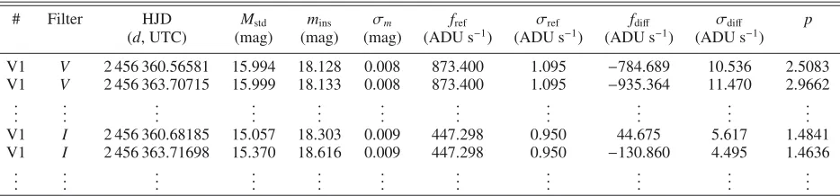
Table 2.Format for the time-series photometry of all confirmed variables in ourV- andI-band CCD observations.

# Filter HJD Mstd mins σm fref σref fdiff σdiff p

(d, UTC) (mag) (mag) (mag) (ADU s−1_{) (ADU s}−1_{) (ADU s}−1_{) (ADU s}−1₎

V1 V 2 456 360.56581 15.994 18.128 0.008 873.400 1.095 −784.689 10.536 2.5083 V1 V 2 456 363.70715 15.999 18.133 0.008 873.400 1.095 −935.364 11.470 2.9662

..

. ... ... ... ... ... ... ... ... ... ...

V1 I 2 456 360.68185 15.057 18.303 0.009 447.298 0.950 44.675 5.617 1.4841 V1 I 2 456 363.71698 15.370 18.616 0.009 447.298 0.950 −130.860 4.495 1.4636

..

. ... ... ... ... ... ... ... ... ... ...

Notes.The standardMstdand instrumentalminsmagnitudes listed in Cols. 4 and 5 correspond to the variable star, filter, and epoch of mid-exposure

listed in Cols. 1–3, respectively. The uncertainty onminsand Mstdis listed in Col. 6. For completeness, we also list the reference flux frefand

the differential flux fdiff (Cols. 7 and 9, respectively), along with their uncertainties (Cols. 8 and 10), as well as the photometric scale factor p.

Definitions of these quantities can be found in e.g.Bramich et al.(2011), Eqs. (2), (3). This is a representative extract from the full table, which is available at the CDS.

of 3.5 pixels; images that already have aFWHM ≥ 3.5 pixels were not blurred. This is to avoid under-sampling, which can cause difficulties in the determination of the DIA kernel solu-tion. Images were stacked from the best-seeing photometrically stable night in order to obtain a high signal-to-noise ratio (S/N) reference image in each filter. If an image had too many sat-urated stars, it was excluded from the reference. The resulting images inV andI are made up of 12 and 20 stacked images, respectively, with combined exposure times of 480 s (inV) and 800s (inI), and respective point-spread function (PSF) FWHM of 3.17 pixels (1.49) and 3.09 pixels (1.45). The reference frames were then used to measure source positions and refer-ence fluxes in each filter. Following this, the images were regis-tered with the reference frame, and the convolution of the refer-ence with the kernel solution was subtracted from each image. This resulted in a set of difference images, from which we ex-tracted difference fluxes for each source, allowing us to build light curves for all of the objects detected in the reference im-ages. The light curves of the variable stars we detected in M 68 are available for download at the CDS, in the format outlined in Table2.

2.2.2. EMCCD observations

Each EMCCD data cube was first pre-processed using the algo-rithms ofHarpsøe et al.(2012), which included bias correction, flatfielding, and alignment of all exposures (corresponding to a tip-tilt correction). This procedure also yielded the point-spread function (PSF) width of each exposure. Each data cube was then subdivided into ten groups of exposures of increasing PSF size.

We then reduced the pre-processed EMCCD cubes using a modified version of theDanDIA pipeline, and a different noise model was adopted to account for the difference between CCD and EMCCD observations, as detailed byHarpsøe et al.(2012). Conventional LI techniques only keep the best-quality expo-sures within a data cube and therefore usually discard most of them, but here we build the reference image from the best-seeing groups alone, but the photometry is measured from all exposures within the data cubes. That is, once a reference image has been built, the full sets of exposures (including the ones with worse seeing) are stacked for each data cube; we do this to achieve the best possible S/N. The sharp reference image is then convolved

with the kernel solution and subtracted from each of the stacked data cubes.

Our EMCCD reference image has a PSF FWHM of 4.5 pixels, or 0.40, and has a total exposure time of 302.4 s (3024×0.1 s).

2.3. Photometric calibration

2.3.1. Self-calibration

For the CCD data, we self-calibrated the light curves to correct for some of the systematics. Although systematics cannot be re-moved completely, substantial corrections can be made in the case of time-series photometry, as shown in our previous papers (e.g.Kains et al. 2013).

We used the method ofBramich & Freudling(2012) to de-rive magnitude offsets to be applied to each epoch of the pho-tometry, which corrected for any errors in the fitted values of the photometric scale factors. The method involves setting up a (linear) photometric model for all of the available photometric measurements of all stars and solving for the best-fit parameter values by minimisingχ2_{. In our case, the model parameters}

con-sist of the star mean magnitudes and a magnitude offset for each image. The offsets we derive are a few percentage points, and they lead to significant improvements in the light curves for this cluster. An illustration of this is shown in Fig.1.

2.3.2. Photometric standards

We used secondary photometric standards in the FOV from Stetson(2000) covering the full range of colours of our CMD to convert the instrumental magnitudes we obtained from the pipeline reduction of the CCD images to standard Johnson-Kron-Cousins magnitudes. This was done by fitting a linear re-lation to the difference between the standard and instrumental magnitudes,mstd−mins, and the instrumentalv−icolour of each

Fig. 1.V-band light curves for V44 before (top) and after (bottom) self-calibration using the method ofBramich & Freudling(2012), showing significant improvement in light curve quality.

2.4. Astrometry

We derived astrometry for our CCD reference images by using Gaia2to match∼300 stars manually with the UCAC3 catalogue (Zacharias et al. 2010). For the EMCCD reference, we derived the transformation by matching ten stars to HST/WFC3 images (e.g.Bellini et al. 2011). The coordinates we provide for all stars in this paper (Table4) are taken from these astrometric fits. The rms of the fit residuals are 0.27 arcsec (0.57 pixel) for the CCD reference images and 0.09 arcsec (0.96 pixel) for the EMCCD reference.

3. Variables in M 68

The first 28 (V1-V28) variables in this cluster were identi-fied by Shapley and Ritchie (Shapley 1919, 1920), using fif-teen photographs obtained with the 60-inch reflector telescope at Mt Wilson Observatory. All of these are RRL stars, except for V27, which was identified in the 1920 paper as a long-period variable.Greenstein et al.(1947) used a spectrum of V27 taken at the McDonald Observatory in 1939 to work out its radial ve-locity and compared this to the cluster’s radial veve-locity to con-clude that V27 is a long-period foreground variable star.Rosino & Pietra(1954) then used observations taken between 1951 and 1953 at Lojano Observatory to derive periods for 20 variables and discovered three additional RRL stars (V29–V31). They also

2 _{http://star-www.dur.ac.uk/~pdraper/gaia/gaia.html}

Fig. 2.Relations used to convert from instrumental to standard Johnson-Kron-Cousins magnitudes for theV(top) andI(bottom) bands.

noted some irregularities in V3, V4, V29, and V30, whereby they could not derive precise periods for those four stars.van Agt & Oosterhoff (1959) found seven more variables (V32–V38) when analysing observations taken in 1950 with the Radcliffe 74-inch reflector telescope in South Africa. They also noticed many discrepancies between their derived periods and those pub-lished a few years earlier byRosino & Pietra(1954), as well as differences in light curve morphologies.Terzan et al.(1973) an-nounced another four variables in M 68 (V39–V42), including the first SX Phe star in this cluster.Clement (1990) and C93 then studied 30 of the RRL stars, identifying nine double-mode pulsators and detecting period changes since the earlier studies. Brocato et al.(1994) carried out the first CCD-era study of this cluster using the 1.5 m ESO Danish Telescope, and soon after, W94 used CCD observations made in 1993 at the CTIO 0.9m telescope in Chile to discover an additional six variables (V43– V48), including another SX Phe star. Finally,Sariya et al.(2014) have recently used observations from 2011 at the Sampurnanand telescope in Nainital, northern India, to claim nine new variable detections, including five RR1 stars, bringing the total number of published variables in this cluster to 57.

3.1. Detection of variables 3.1.1. CCD observations

We searched for variables using two methods: we began by in-specting the difference images visually and checked light curves of any objects that had residuals on a significant number of im-ages. This did not enable us to detect any new variables. We also constructed an image from the sum of the absolute values of all difference images and inspected light curves at pixel positions with significant peaks on this stacked image. As with the first method, this method recovered most known variables, but did not enable us to detect new variables. Finally, we conducted a period search for periods ranging from 0.02 to 2 days on all light curves using the “string length” method (e.g.Dworetsky 1983) and computed the ratioSRof the string length for the best-fit

Table 3.Epochs, periods, mean magnitudes, and amplitudesAinVandIfor all confirmed variable stars in M 68.

# Epoch P β V I AV AI Type

(HJD-2 450 000) (d) [dMyr−1] [mag] [mag] [mag] [mag] RR0

V2 6411.5879 0.5781755 −0.125 15.75 15.17 0.72 0.49 RR0

V9 6412.5455 0.579043 − 15.72 15.12 0.69 0.40 RR0b

V10 6363.7134 0.551920 − 15.71 − 1.08 − RR0b

V12 6369.4311 0.615546 − 15.56 15.04 0.89 0.61 RR0

V14 6373.4455 0.5568499 +1.553 15.73 15.20 1.11 0.77 RR0

V17 6411.5835 0.668424 − 15.68 15.08 0.82 0.54 RR0(b?)

V22 6373.4162 0.5634451 − 15.67 15.13 1.15 0.75 RR0

V23 6410.5710 0.6588921 − 15.68 15.11 1.11 0.58 RR0

V25 6411.5323 0.6414842 −0.488 15.72 15.08 0.79 0.45 RR0b V28 6363.7134 0.6067796 +0.102 15.75 15.14 1.18 0.70 RR0 V30 6370.5680 0.7336375 +0.044 15.64 15.00 0.37 0.25 RR0

V32 − 0.5882 − − − − − RR0

V35 6381.6690 0.7025348 − 15.56 15.00 1.05 0.66 RR0

V46 6363.7743 0.7382510 − 15.64 15.01 0.54 0.37 RR0

RR1

V1 6381.7111 0.3495912 +0.273 15.70 15.23 ∼0.45 0.40 RR1 V5 6366.6697 0.2821009 −0.497 15.72 15.36 0.45 0.28 RR1b V6 6385.6186 0.3684935 −0.088 15.69 15.20 0.53 0.34 RR1 V11 6370.6253 0.3649338 +0.225 15.71 15.24 ∼0.55 0.37 RR1 V13 6411.5829 0.3617370 +0.116 15.74 15.26 0.58 0.36 RR1

V15 6385.6092 0.3722615 − 15.68 15.20 0.53 0.34 RR1

V16 6381.6814 0.3819671 +0.066 15.69 15.22 0.50 0.35 RR1 V18 6363.7943 0.3673459 −0.051 15.72 15.24 0.55 0.37 RR1 V20 6363.7643 0.3857892 +0.234 15.68 15.20 0.56 0.34 RR1 V24 6370.4698 0.3764448 −1.081 15.68 15.20 0.50 0.34 RR1

V33 6385.5693 0.3905647 − 15.67 15.17 0.47 0.23 RR1

V37 6363.7727 0.3846092 − 15.64 15.17 0.47 0.33 RR1

V38 6370.4420 0.3828116 − 15.63 15.17 0.53 0.33 RR1

V43 6363.7527 0.3706144 − 15.71 15.24 0.57 0.35 RR1

V44 6371.4311 0.3850912 − 15.67 15.16 0.48 0.29 RR1

V47 6385.6436 0.3729255 − 15.63 15.13 0.49 0.32 RR1

RR01

V3 6381.6890 0.3907346 − 15.64 15.20 0.68 0.42 RR01

V4 6410.6485 0.3962175 − 15.67 15.20 0.61 0.40 RR01

V7 6381.7511 0.3879608 − 15.71 15.22 0.62 0.41 RR01

V8 6412.5861 0.3904076 − 15.65 15.18 0.53 0.34 RR01

V19 6368.6564 0.3916309 − 15.66 15.18 0.56 0.34 RR01

V21 6385.6233 0.4071121 − 15.62 15.15 0.64 0.42 RR01

V26 6369.4571 0.4070332 − 15.72 15.18 0.80 0.50 RR01

V29 6387.5498 0.3952413 − 15.71 15.14 0.56 0.30 RR01

V31 6385.6217 0.3996599 − 15.58 15.15 0.66 0.43 RR01

V34 6363.7673 0.4001371 − 15.76 15.17 ∼0.60 0.45 RR01

V36 6384.6470 0.415346 − 15.68 15.16 0.64 0.40 RR01

V45 6366.6760 0.3908187 − 15.72 15.17 0.52 0.30 RR01

SX Phe

V39 6433.2863 0.0640464 − 18.04 17.66 0.85 0.64 SX

V48 6387.6218 0.043225 − 17.29 16.93 0.24 ∼0.11 SX

V49 6387.6120 0.048469 − 18.09 17.68 0.59 0.40 SX

V50 6370.4561 0.065820 − 17.56 17.13 0.70 0.30 SXd

V51 6383.6232 0.058925 − 17.24 16.73 0.35 0.20 SX

V52 6410.5871 0.037056 − 17.90 17.51 0.25 ∼0.20 SX

Others

V27 2697.3 322.2342 − 9.8 − 4.03 − Field Mira†

V53 − − − 16.98 15.26 ≥0.1 − ?

Table 4.Equatorial celestial coordinates of all confirmed variables in M 68 at the epoch of the reference image, HJD∼2 456 385.6 d.

# RA Dec

RR0

V2 12:39:15.29 −26:45:24.6 V9 12:39:25.57 −26:44:00.8 V10 12:39:25.96 −26:44:54.7 V12 12:39:26.918 −26:44:39.73 V14 12:39:27.54 −26:41:04.2 V17 12:39:29.02 −26:45:52.4 V22 12:39:32.30 −26:45:01.6 V23 12:39:32.41 −26:38:23.0 V25 12:39:38.15 −26:42:37.2 V28 12:40:00.31 −26:41:59.8 V30 12:39:36.07 −26:45:55.6 V32 12:39:03.29 −26:55:18.0 V35 12:39:25.19 −26:45:32.5 V46 12:39:24.84 −26:44:43.4 RR1

V1 12:39:06.86 −26:42:53.3 V5 12:39:23.83 −26:41:52.3 V6 12:39:23.77 −26:44:23.6 V11 12:39:26.56 −26:46:32.7 V13 12:39:27.49 −26:45:35.9 V15 12:39:28.50 −26:43:40.9 V16 12:39:28.54 −26:43:22.1 V18 12:39:29.12 −26:46:15.2 V20 12:39:30.26 −26:46:33.2 V24 12:39:33.15 −26:44:46.6 V33 12:39:34.41 −26:43:40.7 V37 12:39:26.18 −26:44:20.9 V38 12:39:26.09 −26:45:08.3 V43 12:39:29.06 −26:45:43.7 V44 12:39:29.477 −26:44:38.06 V47 12:39:28.831 −26:44:19.92 RR01

V3 12:39:17.33 −26:43:09.9 V4 12:39:19.06 −26:46:51.3 V7 12:39:24.02 −26:45:57.7 V8 12:39:25.18 −26:46:52.5 V19 12:39:30.15 −26:43:30.4 V21 12:39:31.19 −26:44:32.0 V26 12:39:39.46 −26:45:22.9 V29 12:39:48.93 −26:47:10.1 V31 12:39:19.65 −26:43:05.4 V34 12:39:47.56 −26:41:03.5 V36 12:39:24.89 −26:45:32.1 V45 12:39:29.989 −26:44:49.18 SX Phe

V39 12:39:24.34 −26:44:51.8 V48 12:39:38.27 −26:46:12.4 V49 12:39:29.52 −26:44:09.3 V50 12:39:32.12 −26:45:10.5 V51 12:39:28.986 −26:44:48.47 V52 12:39:30.57 −26:44:30.1 Others

V27 12:39:55.92 −26:40:17.4 V53 12:39:08.91 −26:50:33.8

Notes.More precise coordinates are given for stars within the FOV of the EMCCD reference image, with epoch∼2 456 451 d. The coordi-nates for V32, which is outside of our FOV, are from C93.

light curve scatter, the mean value is around 0.75; for true peri-odic light curves,SR 1. The distribution ofSR is shown in

Fig.3. We inspected all light curves that fell below an arbitrary threshold ofSR=0.5, chosen by visually inspecting light curves

sorted with ascendingSR.

Fig. 3.Distribution of the SR statistic as defined in the text, for our V-band light curves. A dashed line denotes the threshold below which we searched for periodic variables. RR0, RR1, and RR01 variables are shown as red filled circles, green filled triangles, and blue open inverted triangles, respectively. SX Phe is indicated as open green triangles, the field Mira variable V27 (FI Hya) as a filled blue square, and the variable of unknown type V53 as an open green square. The three marked stars above the threshold are V40-V42, which we found to be non-variable.

Table 5.Light curve mean magnitudes and rms values for V40-42, for which we do not find evidence of variability, as well as for the “new” variables published bySariya et al.(2014).

# V rms (V) I rms (I) # [mag] [mag] [mag] [mag] V40 18.32 0.068 17.50 0.075 V41 18.15 0.052 17.36 0.060 V42 19.05 0.083 18.36 0.156 SV49 14.72 0.008 13.67 0.007 SV50 15.15 0.010 14.14 0.008

SV51 12.68 0.013 − −

SV52 18.17 0.225 − −

SV53 18.60 0.077 17.94 0.14 SV54 18.48 0.361 17.00 0.14 SV55 17.04 0.023 16.21 0.03 SV56 19.81 0.192 18.97 0.31 SV57 16.81 0.016 15.91 0.02

Notes.SinceSariya et al.(2014) assigned those variables newV num-bers, we add an “S” as a prefix to avoid confusion with the confirmed variables in this paper.

Using this method, we recovered all known variables except for V32, which is outside our FOV, and we were able to derive periods for all of them, except for V27, which is now known to be a foreground variable star with a period of∼322 d (Pojmanski 2002). For V27, we do not have anI-band light curve because it is saturated in our reference image. We also discovered four new variables, all of them SX Phe stars. Furthermore, we find that V40–42 are not variable within the limits of the rms in our data, given in Table5, in agreement with the findings of W943_.

We also find that none of the new variables recently claimed by Sariya et al.(2014) is variable within the rms scatter of our data (Table5, see also Fig.4), and we therefore continue the variable

3 _{The mean magnitudes of V41 and V42 are significantly different}

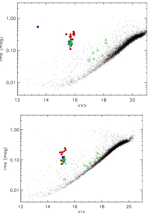
Fig. 4.Root mean square magnitude deviation versus mean magnitude for all stars for which photometry was obtained. Plots are for theV-band (top) and I-band (bottom). Classified variables are marked with red filled circles (RR0), green filled triangles (RR1) and blue open inverted triangles (RR01), green open triangles (SX Phe), a blue square (for V27, the field Mira variable FI Hya), and a green open square (variable V53, of unknown type). Non-variable objects previously catalogued as vari-able in the literature are denoted by red crosses.

numbering system from its standing prior to the publication of their paper.

We also confirm that many of the RRL stars are double-mode variables, as previously reported byClement(1990) and C93, and we determine pulsation periods for both modes, when pos-sible. Double-mode RRL stars in this cluster are discussed in Sect.5.1.

To obtain the best possible period estimate for each star, we used archival data from previous studies of variability in this cluster byRosino & Pietra(1953,1954), C93, W94, andBrocato et al.(1994). This gives us a baseline of up to 62 years for stars that were observed byRosino & Pietra(1953) and over 20 years for the stars that were observed in the 1993–1994 studies. The data ofRosino & Pietra(1953,1954), andBrocato et al.(1994) were previously not available in electronic format, so we up-loaded the light curves to the CDS for interested readers. For some of the stars, it was not possible to phase-fold the data sets without also fitting for a linear period change. For some even this did not lead to well-phased data sets, suggesting that some other effect is at work, such as a non-linear period change. Those are discussed in Sect.3.3.

We also performed frequency analysis on all of the light curves in order to characterise the Blazhko effect (Blažko 1907), which can cause scatter in the phased light curve due to modulation of amplitude, frequency, phase, or a combination of those. We discuss the results of this search in Sect.3.3.

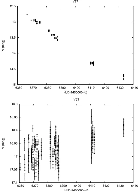
Finally, we inspected the light curve of the standard star S28, which W94 found to be variable with an amplitude of∼0.1 mag. Our data show an increase in brightness of∼0.1 mag as well over the time span of our observations, confirming the variable nature of this star. We therefore assign it the variable number V53. Interestingly, however, we do not find significant variation in theI-band light curve of this star.

TheV-band light curves for all of the variables objects are plotted in Figs.5–9.I-band light curves are available for down-load at the CDS. A finding chart for all confirmed variables in M 68 is shown in Fig.10and a CMD in Fig.11. The CMD con-firms the classification of the confirmed variables, with RRL lo-cated on the instability strip and SX Phe stars in the blue strag-gler region. We also show stamps of variables detected on our EMCCD images ion Fig.12.

3.1.2. EMCCD observations

We repeated the method we used for CCD observations to search for variability in the EMCCD observations we obtained. Of the known variables, only V44 has a light curve, with V12, V45, and V47 also located within our FOV, but is too close to the edge to allow for photometric measurements. Furthermore, the camera was changed in May 2013, with a slightly different filter after that, meaning that measurements from images taken be-fore and after the change need to be treated as separate light curves.

We also detect the new variable V51, and confirm the pe-riod found with the CCD data for this object. The EMCCD light curves for V44 and V51 are shown in Fig.13.

3.2. Period changes in RRL stars

Period changes have been observed in many RRL stars both in the Galactic field and in globular clusters. Period changes are usually classed as evolutionary or non-evolutionary. Evolutionary period changes of stars on the instability strip are understood to be due to their radius increasing and contracting. These only account for slowly increasing or decreasing changes, however, and in many RRL, abrupt period changes have been ob-served (e.g.Stagg & Wehlau 1980), which cannot be explained by such an evolution. As yet, there is no clear explanation for such changes.

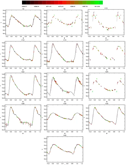
Fig. 5.PhasedV-band light curves of the confirmed RR0 variables in M 68. Data from different nights are plotted in different colours (electronic version only), with a colour bar provided for reference (top panel). On the light curves for which a good Fourier decomposition could be obtained, the fit is overplotted. The size of typical 1σerror bars is plotted in the top left corner. The magnitude scale is the same on all plots in order to facilitate comparison of variation amplitude.

smaller for OosterhoffI clusters than OosterhoffII. Few com-prehensive studies of period changes in cluster RRL have been published:Smith & Wesselink (1977) derived period changes for RRL in the Oosterhoff type II cluster M 15, with a mean ofβ = 0.11±0.36 d Myr−1. For the Oosterhofftype I cluster M 3,Jurcsik et al.(2012) find a slightly positive mean value of

β ∼ 0.01 d Myr−1, agreeing with the theoretical predictions of Lee(1991) and the findings ofRathbun & Smith(1997).

The parameterβis defined such that the period at timetis given by

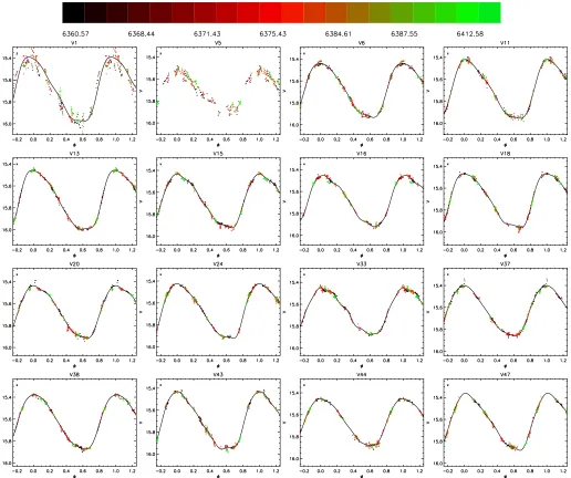
Fig. 6.Same as Fig.5, but for RR1 stars.

whereP0 is the period at the (arbitrary) epochE, andβas

ex-pressed in Eq. (1) is in units of d d−1; however,βis usually ex-pressed in d Myr−1as a more natural unit. The number of cycles NEelapsed at timetsince the epochEcan then be calculated as

NE =

t

E

dx P(x) =

1

βln

1+ β P0

(t−E)

. (2)

The phase is then

φ=NE− NE. (3)

Here we use data stretching back to 1951 (see Sect.3) to derive period changes for RR0 and RR1 stars for which data sets are not well phased and/or are aligned with a single constant period. To do this we performed a grid search in the (P0, β) plane by

min-imising the string length of our data combined with those of W94 (both taken inV-band). We then searched manually around the best-fit solution incorporating other data sets taken in different passbands. As a consistency check, we also calculated period-change parameters using the O–C method. This consists of using an ephemeris to predict the times of maxima in the light curves and then plotting the difference between observed and predicted

times of maxima against time. By fitting a quadratic function to this, a value of β can be derived; two such fits are shown in Fig.14for variables V14 and V28, which produced values ofβconsistent with the values derived using the grid method. The interested reader is referred to the papers of, for instance, Belserene(1964) andNemec et al.(1985) for further details.

We found here that the values we found for β using the O−C method did not always produce well-phased light curves for all data sets. This is most likely due to the small number of observed maxima available for the variables in this cluster. For the cases where the two methods did not agree, we used the value found with the grid search. C93 derived period-change rates by computing periods for their light curves and for archival light curves, and by subtracting one from another. The method used here and the availability of more data mean that our period-change calculations should be more robust. The signs of our val-ues ofβagree with those of C93 except for V2 and V18, which, however, had very large associated error bars in that study.

Fig. 7.PhasedV-band light curves of the RR01 stars. The light curves are phased with the first-overtone pulsation period. A typical 1σerror bar is plotted in the top left corner. The magnitude scale is the same on all plots in order to facilitate comparison of variation amplitude.

evolution of M 68. We find a mean value of β = 0.02± 0.57 d Myr−1_.

3.3. Discussion of individual RRL variables

The RR0 variables are plotted in Fig. 5, RR1 in Fig. 6, and RR01 in Fig.7. Details of period-change calculations are given in Sect.3.2.

– V1: we could only phase the different data sets by including a period-change parameterβ=0.273 d Myr−1_.

– V2: W94 noted that this star features Blazhko modulation, but our light curves do not enable us to confirm this. We found that a negative period change parameterβ=−0.125 d Myr−1_{was needed to phase-fold the various data sets.}

– V5: this star requires a linear period changeβ = −0.497 d Myr−1_{to phase the different data sets; however, the data from}

Fig. 8.PhasedV-band light curves of the confirmed SX Phe stars in M 68, with a typical 1σerror bar plotted in the top left corner. The magnitude scale is the same in all plots to facilitate comparison of variation amplitude.

12.5

13

13.5

14

14.5

15

6360 6370 6380 6390 6400 6410 6420 6430 6440

V (mag)

HJD-2450000 (d) V27

16.8

16.85

16.9

16.95

17

17.05

17.1

6360 6370 6380 6390 6400 6410 6420 6430 6440

V (mag)

HJD-2450000 (d) V53

Fig. 9.UnphasedV-band light curves of the variables V27 (FI Hya) and V53 (unknown type), plotted with 1σerror bars.

– V6: the data fromRosino & Pietra (1954) are not aligned with the other data sets with a constant period.We find a period-change parameter ofβ=−0.088 d Myr−1_{. The light}

curve may suggest some Blazhko modulation, but our data do not allow us to make a strong claim about this.

– V9: our light curve shows Blazhko modulation, as proposed by W94.

– V10: our light curve for this object shows clear Blazhko plitude modulation. Interestingly, W94 found a constant am-plitude but a variable period.

– V11: we could only phase the data sets simultaneously by including a period-change parameterβ=0.225 d Myr−1_.

– V12: we find no evidence of Blazhko modulation for this star, contrary to W94, who found strong cycle-to-cycle variations, but this may be due do the baseline of W94 being longer by ∼50 days.

– V13: we find that including period-change parameter is needed to phase all the light curves; we find β = 0.116 d Myr−1_.

– V14: W94 noted a variation in shape for the bump at mini-mum brightness, which we cannot confirm in our light curve. We also find that a rather large period change parameter

β = 1.553 d Myr−1 _{was needed to phase-fold all the data}

sets (see Fig.15).

– V15: our observations show some slight residual scatter, which might suggest Blazhko modulation; some evidence of similar scatter is visible in the data of W94.

– V16: a period-change parameterβ=0.066 d Myr−1_was

in-cluded to improve the phase-folding of the various data sets.

Fig. 10.Finding chart for the confirmed variable objects in M 68, using ourVreference image. North is up and east to the left. The image size is 8.8×12.26 arcmin, with each stamp 27.6×27.6. A white circle is centred on each variable and labelled with the variable number. The display scale has been modified where necessary to make the source as clear as possible on the stamps, and the location of the variable is also marked with a cross-hair. Stamps from the EMCCD reference image for V12, V44, V45, and V51 are shown in Fig.12.

baseline. However, comparison of our light curve with that of W94 (Fig.16) shows clearly that the amplitude of the light curve is larger in our data set, which might indicate that mod-ulation is present but slow.

– V18, V20, V24: these stars all required the inclusion of a period-change parameter for satisfactory phase-folding of available data sets.

– V25: we find a period-change parameter to phase all the data sets of β = −0.488 d Myr−1_{. The light curve also shows}

Blazhko modulation, as already noted by W94.

Fig. 11.(V−I),Vcolour-magnitude diagram from our photometry. The location of RR0 (red filled circles), RR1 (green filled triangles), RR01 (blue inverted triangles), and SX Phe (open green triangles) stars are shown. The variable V53 (unknown type) is shown as an open green square. Typical error bars are shown for different magnitude levels on the right-hand side of the plot. Aninsetin the top left corner of the plot shows a zoom of the instability strip region of the HB. For added information, isochrones for 9, 10, 11, 12, 13, 14, and 15 Gyr fromDotter et al.(2008) are overplotted in different colours; the best-fit isochrone (13 Gyr) is plotted as a thick green solid line.

– V30: a small positive period-change parameter β = 0.044 d Myr−1_{was found to be needed to phase all data sets.}

– V33: this star is now RR1, but used to be RR01, as first noted by C93. Like C93, we fail to detect signs of the sec-ondary pulsations that were visible in the data ofvan Agt & Oosterhoff(1959).

– V47: we do not confirm the suggestion of W94 that this star is affected by Blazhko modulation, since it may be due to the longer baseline of the W94 data.

4. Fourier decomposition of RR Lyrae star light curves

We performed a Fourier decomposition of the V-band light curves of RRL variables in order to derive several of their prop-erties with well-established empirical relations. We can then use individual stars’ properties to estimate the parameters of the host cluster. Fourier decomposition mean fitting light curves with the Fourier series

m(t)=A0+

N

k₌1

Akcos

2πk

P (t−E)+φk

, (4)

Fig. 12.Stamps from the EMCCD reference image for the stars within our EMCCD FOV, except V47, which is too close to the edge of the image. North is up and east to the left. Each stamp is 3.6×3.6and a cross-hair marks the location of the variable star.

wherem(t) is the magnitude at timet,Nthe number of harmon-ics used in the fit,Pthe period of the variable,Ethe epoch, and Akandφkare the amplitude and phase of thekthharmonic,

re-spectively. The epoch-independent Fourier parameters are then defined as

Ri j = Ai/Aj (5)

φi j = jφi−iφj. (6)

5.8

5.85

5.9

5.95

6

6.05

6.1

-0.2 0 0.2 0.4 0.6 0.8 1 1.2

Magnitude (instrumental)

φ

V44

8.15

8.2

8.25

8.3

8.35

8.4

8.45

-0.2 0 0.2 0.4 0.6 0.8 1 1.2

Magnitude (instrumental)

φ

V51

Fig. 13.EMCCD light curve for variables V44 and V51. See Table3 for information about these variables. For V44 we show the light curves before (blue+signs) and after (red asterisks) the camera change as separate light curves, as discussed in the text. For V51, we show only the light curve after the change because the photometry before was too poor.

curves due to noise. We also checked the sensitivity of the pa-rameters we derived to the number of harmonicsN, and we used only light curves with stable parameters, i.e. ones that showed little variation withN, to estimate cluster parameters. Double-mode pulsators and objects exhibiting signs of Blazhko modula-tion are also excluded from the following analysis.

The Ak coefficients for the first four harmonics and the

Fourier parametersφ21, φ31,andφ41are given in Table6for the

light curves for which we could obtain a Fourier decomposi-tion. We used the deviation parameterDm, defined byJurcsik

& Kovács(1996), as an estimate of the reliability of derived pa-rameters and useDm<5 (e.g.Cacciari et al. 2005) as a selection

criterion. The value ofDmfor each of the successful Fourier

de-compositions is given in Table6.

We did not fit RR0 stars V9, V10, and V25 and RR1 star V5, because they all exhibit Blazhko-type modulation. Furthermore, we did not use the fits of V14, V28, V30, and V46 to derive star properties because those fits have a value ofDm >5. V17

was not fitted either because the parameters varied significantly with the number of harmonics used in the fit, as well as showing signs of slow amplitude modulation (see Sect.3.3). This leaves us with 5 RR0 and 15 RR1 stars for which we derive individual properties in the next section. We also note that for V1, V2, V14, V23, and V30, we combined our data with that of W94 in order to derive fits, owing to insufficient phase coverage of our data alone.

Fig. 14.O–C plots for variables V14 and V28 showing the quadratic fit to the time dependence of the difference between observed and predicted times of light curve maxima. The values found using this quadratic fit for V14 and V28 are consistent with those derived us-ing our grid fittus-ing method (see text),β= +1.553 d Myr−1 _{(V14) and}

β= +0.102 d Myr−1_(V28).

4.1. Metallicity

In this section we derive metallicities for each variable for which a good Fourier decomposition, according to our selection criteria discussed above, could be obtained. To do this, we use empirical relations from the literature. For RR0 stars, we used the rela-tion ofJurcsik & Kovács(1996), which expresses [Fe/H] as a function of the period and of the Fourier parameterφs

31. The s

superscript denotes thatJurcsik & Kovács(1996) derived their relations usingsineseries, whereas we fit cosine Fourier series (Eq. (4)). The Fourier parameters can be easily converted using the equation

φs

i j=φi j−(i−j)π

2· (7)

[Fe/H] can then be expressed as

[Fe/H]J=−5.038−5.394P+1.345φ31s , (8)

15

15.5

16

16.5

-0.2 0 0.2 0.4 0.6 0.8 1 1.2

Magnitude (arbitrary)

φ V14

15

15.5

16

16.5

-0.2 0 0.2 0.4 0.6 0.8 1 1.2

Magnitude (arbitrary)

φ V18

Fig. 15.Phased light curves for V14 (top) and V18 (bottom), showing the data sets of this paper (black,+symbols), W94 (green asterisks), C93 (red crosses), and Rosino & Pietra (1954, blue squares). The light curves were phased using a period change of+1.553 d Myr−1_{(V14) and}

−0.051 d Myr−1_(V18).

15.1

15.2

15.3

15.4

15.5

15.6

15.7

15.8

15.9

16

16.1

-0.2 0 0.2 0.4 0.6 0.8 1 1.2

Magnitude (arbitrary)

φ

V17

Fig. 16.Phased light curves for V17, showing theV-band data sets of this paper (black,+symbols) and W94 (green asterisks). The amplitude is larger in our data by∼0.15 mag compared to the observations of W94; we suggest that this might be due to slow amplitude modulation.

metallicity scale ofZinn & West(1984, hereafter ZW) via the simple relation fromJurcsik(1995),

[Fe/H]ZW=

[Fe/H]J−0.88

1.431 · (9)

Kovács (2002) investigated the validity of this relation and found that Eq. (8) yields metallicity values that are too high by∼0.2 dex for metal-poor clusters. This was supported by the findings ofGratton et al. (2004) andDi Fabrizio et al.(2005), who compared metallicity values for RRL stars in the Large Magellanic Cloud (LMC) using both spectroscopy and Fourier decomposition. We therefore include a shift of−0.20 dex (on the [Fe/H]Jscale) or−0.14 dex (on the ZW scale) to the metallicity

values derived for RR0 stars using Eq. (8).

More recently,Nemec et al.(2013) have derived a relation for the metallicity of RR0 stars, using observations of RRL taken with theKeplerspace telescope,

[Fe/H]UVES=b0+b1P+b2φ31s +b3φ31s P+b4

φs

31

2

, (10)

where [Fe/H]UVES is the metallicity on the widely used scale

ofCarretta et al.(2009a), and the constant coefficients were de-termined byNemec et al.(2013) asb0 = −8.65±4.64,b1 =

−40.12±5.18,b3=6.27±0.96,andb4=−0.72± −0.72±0.17.

The scale ofCarretta et al. (2009a) was derived using spectra of red giant branch (RGB) stars obtained using GIRAFFE and UVES. ZW metallicity values can be transformed to that scale (hereafter referred to as the UVES scale) using

[Fe/H]UVES=−0.413+0.130 [Fe/H]ZW−0.356 [Fe/H]ZW2.

(11) In the discussion that follows, we considered RR0 metallicity values obtained both with the scale ofJurcsik & Kovács(1996) and that ofNemec et al.(2013)4_{. For the RR1 variables, we used}

the relation of Morgan et al.(2007) to derive metallicity val-ues.This relates [Fe/H],P,andφ31as

[Fe/H]ZW = 2.424−30.075P+52.466P2 (12)

+0.982φ31+0.131φ231−4.198φ31P.

Metallicity values calculated using Eqs. (8), (9), and (12) are listed in Table7. We note that the metallicities of only two RRL stars in M 68 have previously been measured in the literature. Smith & Manduca(1983) measured the spectroscopic metallic-ity indexΔS for the RR0-type variables V2 and V25 as 11.0 and 10.5, respectively, which yield metallicities [Fe/H]ZW ≈ −2.15

and−2.07, respectively, when converted to the ZW scale via the following relation fromSuntzeffet al.(1991):

[Fe/H]ZW=−0.158ΔS−0.408. (13)

We include these metallicity measurements as a footnote to Table7for the sake of completeness.

4.2. Effective temperature

Jurcsik(1998) derived empirical relations to calculate the eff ec-tive temperature of fundamental-mode RRL stars, relating the (V−K)0 colour toPand to several of the Fourier coefficients

and parameters:

(V−K)0 = 1.585+1.257P−0.273A1−0.234φs₃₁ (14)

+0.062φ₄₁s

logTeff = 3.9291−0.1112 (V−K)0 (15)

−0.0032 [Fe/H]J.

4 _{However, we calculated errors on metallicity values derived from the}

Table 6.Parameters from the Fourier decomposition.

# A0 A1 A2 A3 A4 φ21 φ31 φ41 N Dm

RR0

V2 15.749(2) 0.281(2) 0.086(2) 0.057(2) 0.042(2) 4.031(17) 8.039(23) 6.073(32) 9 4.34 V12 15.559(2) 0.325(2) 0.145(2) 0.113(2) 0.075(2) 3.870(10) 7.940(12) 5.774(19) 11 3.11 V14 15.732(2) 0.421(2) 0.154(3) 0.116(3) 0.068(3) 3.926(13) 7.926(18) 5.765(27) 10 5.04 V22 15.670(2) 0.424(2) 0.179(2) 0.136(2) 0.100(2) 3.836(9) 7.780(13) 5.717(18) 11 2.36 V23 15.678(3) 0.338(3) 0.159(3) 0.118(3) 0.078(3) 3.899(20) 8.157(28) 6.163(40) 8 1.83 V28 15.751(2) 0.371(2) 0.178(2) 0.146(2) 0.076(2) 3.842(8) 8.363(11) 6.064(17) 8 6.44 V30 15.637(2) 0.165(2) 0.059(2) 0.029(2) 0.011(2) 4.121(24) 8.510(43) 7.114(104) 7 17.59 V35 15.562(2) 0.338(2) 0.163(2) 0.113(2) 0.081(2) 4.041(8) 8.411(11) 6.478(14) 9 2.87 V46 15.637(2) 0.209(2) 0.091(2) 0.055(2) 0.026(3) 4.090(25) 8.684(35) 7.187(47) 10 7.94 RR1

V1 15.700(2) 0.296(3) 0.059(3) 0.023(3) 0.016(3) 4.558(39) 2.581(93) 1.461(125) 4 − V6 15.691(1) 0.251(1) 0.040(2) 0.021(1) 0.009(1) 4.619(15) 2.962(31) 2.102(73) 4 − V11 15.706(1) 0.265(2) 0.052(2) 0.025(2) 0.007(2) 4.554(13) 2.521(25) 1.837(78) 4 V13 15.742(1) 0.274(2) 0.049(2) 0.028(2) 0.013(2) 4.536(15) 2.722(23) 1.066(47) 5 − V15 15.684(1) 0.241(1) 0.041(2) 0.019(2) 0.007(2) 4.636(15) 3.074(29) 1.883(73) 5 − V16 15.691(1) 0.229(2) 0.039(2) 0.023(2) 0.001(2) 4.706(16) 2.865(31) 1.936(410) 6 − V18 15.722(1) 0.249(2) 0.046(2) 0.027(2) 0.015(2) 4.566(15) 2.873(24) 1.930(48) 4 − V20 15.676(1) 0.239(1) 0.036(1) 0.019(2) 0.004(1) 4.806(15) 3.129(27) 2.355(126) 5 − V24 15.682(2) 0.247(2) 0.048(2) 0.022(2) 0.011(2) 4.637(17) 2.894(35) 1.978(68) 6 − V33 15.670(1) 0.211(2) 0.030(2) 0.013(2) 0.006(2) 4.627(23) 2.983(51) 2.787(115) 6 − V37 15.641(1) 0.227(2) 0.036(2) 0.011(2) 0.006(2) 4.392(21) 3.013(59) 2.440(98) 4 − V38 15.631(1) 0.250(2) 0.038(2) 0.016(2) 0.006(2) 4.537(16) 3.180(37) 2.052(93) 4 − V43 15.713(1) 0.261(2) 0.048(2) 0.021(2) 0.011(2) 4.439(17) 2.408(35) 1.378(62) 5 − V44 15.672(2) 0.216(2) 0.032(2) 0.012(2) 0.004(2) 4.706(31) 3.205(62) 1.854(147) 5 − V47 15.629(2) 0.248(2) 0.048(2) 0.016(2) 0.007(2) 4.645(21) 2.799(62) 2.676(123) 5 −

Notes.Numbers in parentheses are the 1σuncertainties on the last decimal place.

Simon & Clement(1993) used theoretical model to derive a cor-responding relation for RR1 stars,

logTeff =3.7746−0.1452 logP+0.0056φ31. (16)

We use those relations to derive logTeff for all of our RR0 and

RR1 stars, and give the resulting values in Table7. As men-tioned in previous analyses (e.g. Arellano Ferro et al. 2008), there are some important caveats to consider when estimating temperatures with Eqs. (15) and (16). The values of logTefffor

RR0 and RR1 stars are on different absolute scales (e.g.Cacciari et al. 2005), and temperatures derived using these relations show systematic deviations from those predicted byCastelli (1999) in their evolutionary models or on the temperature scales of Sekiguchi & Fukugita(2000). However, we use them in order to have a comparable approach to the one taken in our previous studies of clusters.

4.3. Absolute magnitude

We used the empirical relations ofKovács & Walker(2001) to deriveV-band absolute magnitudes for the RR0 variables, MV =−1.876 logP−1.158A1+0.821A3+K0, (17)

whereK0 is the zero point of the relation. Using the absolute

magnitude of the star RR Lyrae ofMV =0.61±0.10 mag derived

byBenedict et al.(2002) and a Fourier decomposition of its light curve,Kinman (2002) determined a zero point for Eq. (17) of K0 = 0.43 mag. Here, however, we adopt a slightly different

value ofK0 = 0.41±0.02 mag, as in several of our previous

studies (e.g.Arellano Ferro et al. 2010), in order to maintain consistency with a true distance modulus ofμ0 =18.5 mag for

the LMC (Freedman et al. 2001). A nominal error of 0.02 mag onK0 was adopted in the absence of uncertainties onK0 in the

literature.

For RR1 variables, we use the relation ofKovács(1998),

MV =−0.961P−0.044φs₂₁−4.447A4+K1, (18)

where we adopted the zero-point value ofK1 = 1.061±0.020

mag (Cacciari et al. 2005), with the same justification as for our choice ofK0.

We also converted the magnitudes we obtained to luminosi-ties using

log (L/L)=−0.4 MV+BC(Teff)−Mbol, , (19)

whereMbol,is the bolometric magnitude of the Sun,Mbol, =

4.75 mag, and BC(Teff) is a bolometric correction that we

es-timate by interpolating from the values of Montegriffo et al. (1998) for metal-poor stars, and using the value of logTeff we

derived in the previous section. Values of MV and log(L/L)

for the RR0 and RR1 variables are listed in Table 7. Using our average values ofMV, in conjunction with the average

val-ues of [Fe/H]ZW (Sect.4.1), we find good agreement with the

MV−[Fe/H]ZWrelation derived in the literature (e.g.Kains et al.

Table 7.Physical parameters for the RRL variables calculated using the Fourier decomposition parameters and the relations given in the text.

# [Fe/H]ZW [Fe/H]UVES MV log(L/L) logTeff

RR0

V2 −1.85(2) −2.17(6) 0.578(30) 1.679(12) 3.804(2) V12 −2.09(1) −2.81(3) 0.522(24) 1.704(10) 3.800(2) V22 −2.04(1) −2.72(4) 0.498(27) 1.709(11) 3.807(2) V23 −2.04(3) −2.58(8) 0.455(27) 1.733(11) 3.797(2) V35 −1.97(1) −2.21(3) 0.399(30) 1.758(12) 3.795(2) RR1

V1 −2.06(3) − 0.521(23) 1.658(10) 3.855(2) V6 −2.06(2) − 0.533(21) 1.655(9) 3.854(1) V11 −2.12(1) − 0.548(21) 1.650(9) 3.852(1) V13 −2.08(1) − 0.524(21) 1.658(9) 3.854(1) V15 −2.05(2) − 0.538(21) 1.653(9) 3.854(1) V16 −2.11(1) − 0.550(21) 1.650(9) 3.851(1) V18 −2.07(1) − 0.511(21) 1.664(9) 3.854(1) V20 −2.08(1) − 0.529(21) 1.658(9) 3.852(1) V24 −2.10(2) − 0.517(21) 1.663(9) 3.852(1) V33 −2.11(2) − 0.526(21) 1.661(9) 3.851(1) V37 −2.10(2) − 0.540(21) 1.654(9) 3.852(1) V38 −2.06(2) − 0.536(21) 1.655(9) 3.853(1) V43 −2.14(1) − 0.531(21) 1.658(9) 3.851(1) V44 −2.07(2) − 0.533(21) 1.656(9) 3.853(1) V47 −2.10(2) − 0.536(21) 1.655(9) 3.852(1)

Notes.Numbers in parentheses are the 1σuncertainties on the last decimal place. The values of [Fe/H]UVESlisted in this table for RR0 stars

are derived using the relation ofNemec et al.(2013). In addition, we note thatSmith & Manduca(1983) found [Fe/H]ZW ≈ −2.15 for V2 and

[Fe/H]ZW≈ −2.07 for V25, using theΔS method (see Sect.4.1). Errors quoted for logTeffare only statistical and not systematic; we could not

calculate systematic errors for logTeffas no errors are given on the empirical coefficients in Eqs. (15) and (16). Errors onMV and log(L/L) for

RR1 stars are dominated by the error on the zero pointK0in Eq. (18).

4.4. Masses

Empirical relations also exist to derive masses of RRL stars from the Fourier parameters, although as noted bySimon & Clement (1993), such relations are better suited to deriving average values for RRL stars in clusters. We therefore use mean parameters to derive mean masses for our RRL stars. For RR0 stars, we use the relation ofvan Albada & Baker(1971),

log(M/M)=16.907−1.47 log(P)+1.24 log(L/L)

−5.12 logTeff, (20)

where we use the symboldMto denote masses to avoid confu-sion with absolute magnitudes elsewhere in the text. Using this, we find an average massMRR0/M=0.74±0.14.

For RR1 stars, we used the relation derived by Simon & Clement(1993) from hydrodynamic pulsation models,

log(M/M)=0.52 logP−0.11φ31+0.39, (21)

which yield a mean mass MRR1/M = 0.70±0.05. This

is lower than the value of M/M = 0.79 found by Simon & Clement (1993) for M 68, but it confirms the value of M/M=0.70±0.01 found by W94 using the same method.

5. Double-mode pulsations

5.1. RR Lyrae

M 68 contains 12 identified double-mode RRL (RR01) stars. RR01 stars are of particular interest, because given metal-licity measurements, the double-mode pulsation provides us with a unique opportunity to measure the mass of these ob-jects without assuming a stellar evolution model and to study the mass-metallicity distribution of field and cluster RRL stars

(e.g. Bragaglia et al. 2001). “Canonical” RR01 have first-overtone-to-fundamental pulsation period ratios ranging from ∼0.74 to 0.75 (e.g.Soszy´nski et al. 2009) for radial pulsations. Other period ratios can be interpreted as evidence for non-radial pulsation or for higher-overtone secondary pulsation, with stud-ies reporting a period ratio of∼0.58–0.59 between the second overtone and the fundamental radial pulsation (e.g.Poretti et al. 2010).

We analysed the light curves of RR01 stars in our images us-ing the time-series analysis softwarePeriod04(Lenz & Breger 2005). In Table8, we list the periods we found for each variable, as well as the period ratio. We found ratios within the range of canonical value for all stars except for V45, for which we did not detect a second pulsation period, unlike W94.

In the past, theoretical model tracks and the “Petersen” dia-gram (P1/P0vs.P0,Petersen 1973) have been used to estimate

the masses of RR01 pulsators. Using this approach, W94 esti-mated average RR01 masses of∼0.77Mand∼0.79Mwith the models ofCox(1991) andKovacs et al.(1991), respectively. Here we use the new relation ofMarconi et al.(2015), who used new non-linear convective hydrodynamic models to derive a re-lation that links the stellar mass with the period ratio and the metallicity, through

log (M/M)=(−0.85±0.05)−(2.8±0.3) log (P1/P0)

−(0.097±0.003) logZ. (22) To convert metallicities from [Fe/H]ZW toZ, we used the

rela-tion ofSalaris et al.(1993),

logZ=[Fe/H]ZW−1.7+log(0.638f+0.362), (23)

Table 8.Fundamental and first-overtone pulsation periods and the period ratio for the double-mode RRL detected in M 68.

# P1[d] A1 P0[d] A0 P1/P0 M/M

V3 0.3907346 0.206 0.523746 0.101 0.7460 0.789±0.119 V4 0.3962175 0.205 0.530818 0.111 0.7464 0.787±0.118 V7 0.3879608 0.201 0.520186 0.107 0.7458 0.789±0.119 V8 0.3904076 0.219 0.522230 0.046 0.7476 0.784±0.118 V19 0.3916309 0.202 0.525259 0.061 0.7456 0.790±0.119 V21 0.4071121 0.221 0.545757 0.138 0.7460 0.789±0.119 V26 0.4070332 0.200 0.546782 0.147 0.7444 0.793±0.120 V29 0.3952413 0.236 0.530525 0.023 0.7450 0.792±0.119 V31 0.3996599 0.200 0.535115 0.121 0.7469 0.786±0.118 V34 0.4001371 0.187 0.537097 0.050 0.7450 0.792±0.119 V36 0.415346 0.203 0.557511 0.106 0.7450 0.792±0.119

V45 0.3908187 0.224 − − − −

Notes.Also listed are semi-amplitudes for each pulsation mode.

[Fe/H]ZW=−2.07±0.06 corresponding to the mean metallicity

of the RRL stars listed in Table7. Using Eqs. (22) and (23), we find the masses given in Table8and a mean mass for RR01 stars ofM/M =0.789±0.003 (statistical)±0.119 (systematic), in excellent agreement with the findings of W94.

5.2. SX Phoenicis

We also carried out a search for double-mode pulsation in the light curves of the SX Phe stars in our sample. For V50, we find a second pulsation periodP1 = 0.051745 d in

addi-tion to the fundamental periodP0 = 0.065820 d, giving a

ra-tioP1/P0 ∼ 0.786 within the range of expected values for a

metal-poor double-radial-mode SX Phe star (Santolamazza et al. 2001). This is confirmed by the location of that secondary pe-riod on the logP−V0 diagram, which is discussed further in

Sect.6.4.2.

6. Cluster properties from the variable stars

6.1. Oosterhoff type

To determine the Oosterhoff type of this cluster, we calculate the mean periods of the fundamental-mode RRL, as well as the ratio of RR1 to RR0 stars. We find PRR0 = 0.63±0.07 d

andPRR1 = 0.37±0.02 d. RR1 stars make up 54% of the

single-mode RRL stars. Although PRR0 is somewhat lower

than the usual canonical value of∼0.68, these values, as well as the very low metallicity, point to M 68 being an Oosterhoff II cluster, in agreement with previous classifications (e.g.Lee & Carney 1999). As mentioned earlier, the fact that M 68 is a clear OosterhoffII type disagrees with studies concluding that M 68 could have an extragalactic origin (e.g.Yoon & Lee 2002), since globular clusters in satellite dSph galaxies of the Milky Way fall mostly within the gap between OosterhoffTypes I and II.

Plotting the RRL stars on a “Bailey” diagram (logP−A, whereAdenotes the amplitude of the RRL light curve; Fig.17) also allows us to confirm the OostheroffII classification, by com-paring the location of our RRL stars to the analytical tracks de-rived by Zorotovic et al. (2010) by fitting the loci of normal and evolved stars of Cacciari et al. (2005). Figure 17 shows that the locations of our RRL stars are in good agreement with these tracks (for theVband) and those ofKunder et al.(2013b) (who rescaled those tracks for theIband). However, it is obvious from theI-band plot (bottom panel of Fig.17) that the RRL loci for M 68 are different from those of OosterhoffType-II clusters

Table 9.Different metallicity estimates for M 68 in the literature.

Reference [Fe/H]ZW [Fe/H]UVES Method

This work −2.07±0.06 −2.20±0.10 Fourier decomposition of RRL light curves This work −2.09±0.26 −2.24±0.42 MV-[Fe/H] relation

Carretta et al.(2009b) −2.10±0.04 −2.27±0.07 UVES spectroscopy of red giants Carretta et al.(2009c) −2.08±0.04 −2.23±0.07 FLAMES/GIRAFFE spectra of red giants Rutledge et al.(1997) −2.11±0.03 −2.27±0.05 CaII triplet

Harris(1996) −2.23 −2.47 Globular cluster catalogue Suntzeffet al.(1991) −2.09 −2.24 Spectroscopy of RR Lyrae/ ΔS index Gratton & Ortolani(1989) −1.92±0.06 −1.97±0.09 High-resolution spectroscopy

Minniti et al.(1993) −2.17±0.05 −2.37±0.08 FeI and FeII spectral lines Zinn & West(1984) −2.09±0.11 −2.24±0.18 Q39index

Zinn(1980) −2.19±0.06 −2.41±0.10 Q39index

Notes.Values were converted using Eq. (11) where necessary.

NGC 5024 (Arellano Ferro et al. 2011) and M 9 (Arellano Ferro et al. 2013a), but agree with the loci for NGC 2808 (Kunder et al. 2013b).

6.2. Cluster metallicity

AlthoughClement et al.(2001) found a correlation between the metallicity of a globular cluster and the mean period of its RR0 stars, PRR0, they note that this relation does not hold when

PRR0 is larger than 0.6 d, i.e. for OosterhoffType-II clusters.

Instead, we estimate the metallicity of M 68 by calculating the average of the metallicities we derived for RRL stars in this cluster. As in our previous papers (e.g.Kains et al. 2013), we assume that there is no systematic offset between the metallici-ties derived for RR0 and RR1 stars. Using this method, we find a mean metallicity of [Fe/H]ZW = −2.07±0.06 (using Eq. (9)

to derive RR0 metallicities) and [Fe/H]ZW =−2.13±0.11

(us-ing Eq. (10)), corresponding to [Fe/H]UVES=−2.20±0.10 and

[Fe/H]UVES=−2.30±0.17,respectively. Both values are in

ex-cellent agreement with the value ofCarretta et al.(2009b), who find [Fe/H]UVES =−2.27±0.01±0.07 (statistical and

system-atic errors, respectively) and with most values in the literature, listed in Table9. In the rest of this paper, we use [Fe/H]ZW =

−2.07±0.06 as the cluster metallicity, owing to the larger scatter in RR0 metallicities derived using Eq. (10) and to the problem with uncertainties in the relation ofNemec et al.(2013) already mentioned in Sect.4.1.

6.3. Reddening

Individual RR0 light curves can be used to estimate the red-dening for each star, using their colour near the point of min-imum brightness. The method was first proposed by Sturch (1966) and further developed in several studies, most re-cently byGuldenschuh et al.(2005) and Kunder et al.(2010). Guldenschuh et al.(2005) find that the intrinsic (V−I)0 colour

of RR0 stars between phases 0.5 and 0.8 is (V −I)φ₀[0.5−0.8] = 0.58±0.02 mag. By calculating the (V −I) colour for each of our light curves between those phases and comparing it to the value ofGuldenschuh et al. (2005), we can therefore cal-culate values ofE(V −I), which we can then convert through E(B−V) =E(V −I)/1.616 (e.g.Arellano Ferro et al. 2013a). Stars showing Blazhko modulation were excluded from this cal-culation, as were stars with poorI−band light curves, leading to reddening estimates for V2, V12, V14, V22, V23, V35, and V46. We found a mean reddening of 0.05±0.05 mag, within the range of values published (see Sect.6.4.1).

6.4. Distance

6.4.1. Using the RRL stars

The Fourier decomposition of RRL stars can also be used to de-rive a distance modulus to the cluster. The Fourier fit parameter A0corresponds to the intensity-weighted meanV magnitude of

the light curve, and since we also derived absolute magnitudes for each star with a good Fourier decomposition, this can be used to calculate the distance modulus to each star.

For RR0 stars, the mean value ofA0 is 15.64±0.08 mag,

while the mean absolute value isMV=0.49±0.07 mag. From

this, we find a distance modulusμ=15.15±0.11 mag. For RR1 stars, we findA0=15.68±0.03 mag andMV=0.53±0.01

mag, yieldingμ=15.15±0.03 mag.

Many values of E(B−V) have been published for M 68, ranging from 0.01 mag (e.g. Racine 1973) to 0.07 mag (e.g. Bica & Pastoriza 1983). Recent studies have tended to use E(B−V) = 0.05 mag, which is the value listed in the cata-logue ofHarris(1996).Piersimoni et al.(2002) derived a value ofE(B−V) =0.05±0.01 fromBV Iphotometry of RRL stars and empirical relations, and this coincides with the value we derived in Sect.6.3, although uncertainties on our estimate are greater. We therefore adopt the value ofPiersimoni et al.(2002) and a value ofRV =3.1 for the Milky Way. From this we find

true distance moduli ofμ0 =15.00±0.11 mag from RR0 stars

andμ0=15.00±0.05 mag from RR1. These values correspond

to physical distances of 10.00±0.49 kpc and 9.99±0.21 kpc, respectively, and are consistent with values reported in the liter-ature, examples of which we list in Table10.

6.4.2. Using SX Phoenicis stars

We can derive distances to SX Phe stars thanks to empirical period-luminosity (P−L) relations (e.g.Jeon et al. 2003). Here we calculate distances to the SX Phe stars in our images (see Table3) using theP−Lrelation ofCohen & Sarajedini(2012), MV =−(1.640±0.110)−(3.389±0.090) logPf, (24)

wherePf is the fundamental-mode pulsation period. This