Design optimization of composite structures operating in acoustic environments

Design optimization of composite structures operating in acoustic environments

D. Chronopoulosa

a_{Institute for Aerospace Technology, The University of Nottingham, NG7 2RD, UK}

Abstract

The optimal mechanical and geometric characteristics for layered composite structures subject to vibroacoustic

exci-tations are derived. A Finite Element description coupled to Periodic Structure Theory is employed for the considered

layered panel. Structures of arbitrary anisotropy as well as geometric complexity can thus be modelled by the

pre-sented approach. Damping can also be incorporated in the calculations. Initially, a numerical continuum-discrete

approach for computing the sensitivity of the acoustic wave characteristics propagating within the modelled periodic

composite structure is exhibited. The first and second order sensitivities of the acoustic transmission coefficient ex-pressed within a Statistical Energy Analysis context are subsequently derived as a function of the computed acoustic

wave characteristics. Having formulated the gradient vector as well as the Hessian matrix, the optimal mechanical and

geometric characteristics satisfying the considered mass, stiffness and vibroacoustic performance criteria are sought by employing Newton’s optimization method.

Keywords: Structural design optimization, Vibroacoustic response, Composite structures, Wave propagation

[Table 1 about here.]

1. Introduction

Layered and complex structures are nowadays widely used within the aerospace, automotive, construction and

energy sectors with a general increase tendency, mainly because of their high stiffness-to-mass ratio and the fact that their mechanical characteristics can be designed to suit the particular purposes. Unluckily however, this high

stiffness-to-mass ratio being responsible for the increased mechanical efficiency, at the same time induces high acous-tic transmission through the structure. The need for simultaneously optimising an industrial structure of minimum

mass and maximum static stiffness, while attaining satisfactory dynamic response performance levels is a challenging task for the modern engineer; especially when considering acoustic transmission through a layered structure which

depends on the mechanical and geometric characteristics of each individual layer, resulting in a great number of design

parameters to be optimised.

The numerical analysis of wave propagation within periodic structures was firstly considered in [1], while the work

was extended to two dimensional media in [2]. The so called Wave Finite Element (WFE) method was introduced in

[3, 4] in order to facilitate the post-processing of the eigenproblem solutions and further improve the computational

efficiency of the method. The interest in predicting the vibroacoustic response of a structure in a wave context is far from being new with the pioneering works of the authors in [5, 6, 7, 8] being probably the earliest ones. A

layer-wise model for the prediction of acoustic wave propagation within continuous layered structures was presented in [9].

More recently, the prediction of the acoustic wave characteristics based on FE formulations allowed for more complex

structures to be included in the acoustic transmission computations [10, 11, 12].

Structural sensitivity analysis is of great importance for understanding the overall impact of a design parameter

variation to the performance characteristics which are to be optimised. Accurate sensitivity models are an

impor-tant tool for design optimization, system identification as well as for statistical mechanics analysis. Several authors

[13, 14, 15, 16] have been focusing on the eigenvalue derivative analysis of a structural system. With regard to the

variability analysis of the waves travelling within a structural medium, the available published work is mainly focused

on deriving expressions [17, 18] of the stochastic wave parameters from analytical models. In [19] the authors conduct

a design sensitivity analysis by a wave based approach. Considering numerical approaches, the authors in [20] used

Bloch’s theorem in conjunction with the FE method in order to calculate the sensitivity of the acoustic waves within

an auxetic honeycomb, while with regard to the computation of the variability of the propagating waves, the authors

in [21, 22] have presented a stochastic WFE approach for computing the variability of wave propagation properties in

one dimensional media. With regard to optimising the design characteristics of a layered structure the developed

ap-proaches have generally focused on genetic algorithms or particle swarm type techniques [23, 24, 25]. When it comes

to optimising the structural design vis-a-vis the dynamic response performance of a structure, wave based optimization

techniques have been developed [26, 27, 28, 29] by adopting Periodic Structure Theory (PST) assumptions.

In this work an established wave based SEA approach is employed in order to predict the vibroacoustic

per-formance of a composite layered panel. The novelty of the work focuses on the derivation of the first and second

order sensitivity of the acoustic transmission coefficient expressed through SEA with respect to the structural design characteristics of the modelled structure. The considered design parameters include the entirety of the mechanical

characteristics, the density as well as the thickness of each individual structural layer. Non conservative structural

systems are also modelled by the exhibited approach. Employing a three dimensional FE description of the modelled

structure allows for capturing the entirety of the sound transmitting propagating structural waves, while employing a

PST formulation allows for drastically reducing the computational cost related to calculating the SEA parameters and

the Hessian matrix for each configuration. Although not discussed in this work, the method is straightforward to apply

to curved structures by expressing the FE structural matrices and wave propagation properties in polar coordinates.

The paper is organized as follows: In Sec.2 the formulation of the sensitivity of the waves propagating within the

periodic structure is elaborated. The PST to be employed is exhibited and the parametric sensitivity of the propagating

waves with regard to the design of the modelled composite panel is deduced. Both conservative and non-conservative

structural systems are considered. In Sec.3 the SEA model for computing the vibroacoustic performance of the layered

The principal SEA quantities, namely the modal density, the radiation efficiency and the intrinsic damping loss factor are all considered. Once the parametric sensitivity of the vibroacoustic performance of the structure is computed, the

formulation of the optimization problem, including the objective function as well as the corresponding Hessian matrix

are formulated in Sec.4. In Sec.5 the presented approach is applied to a layered sandwich asymmetric structure and

the corresponding numerical results are discussed. Conclusions on the presented work are eventually given in Sec.6.

2. Acoustic wave sensitivity

2.1. Formulation of the PST for an arbitrary structural segment

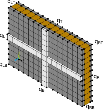
A periodic segment of a panel having arbitrary layering is hereby considered (see Fig.1) with Lx, Lyits dimensions

in the x and y directions respectively. The segment is modelled using a conventional FE software. The mass, damping

and stiffness matrices of the segmentM,CandKare extracted and the DoF set q is reordered according to a predefined sequence such as:

q={qI qB qT qL qR qLB qRB qLT qRT}⊤ (1)

corresponding to the internal, the interface edge and the interface corner DoF (see Fig.1). The free harmonic vibration

equation of motion for the modelled segment is written as:

[K+iωC−ω2_{M]q=0 (2)}

[Figure 1 about here.]

The analysis then follows as in [10] with the following relations being assumed for the displacement DoF under

the passage of a time-harmonic wave:

qR=e−iεxqL, qT=e−iεyqB

qRB=e−iεxqLB, qLT=e−iεyqLB, qRT=e−iεx−iεyqLB

(3)

withεxandεythe propagation constants in the x and y directions related to the phase difference between the sets of

DoF. The wavenumbers kx, kyare directly related to the propagation constants through the relation:

εx=kxLx, εy=kyLy (4)

q=                                                                

I 0 0 0

0 I 0 0

0 Ie−iεy _{0 0}

0 0 I 0

0 0 Ie−iεx ₀

0 0 0 I

0 0 0 Ie−iεx

0 0 0 Ie−iεy

0 0 0 Ie−iεx−iεy

                                                               

x=Rx (5)

with x the reduced set of DoF: x = {qI qB qL qLB}⊤. The equation of free harmonic vibration of the modelled

segment can now be written as:

[R∗KR+iωR∗CR−ω2R∗MR]x=0 (6)

with∗_{denoting the Hermitian transpose. The most practical procedure for extracting the wave propagation}

character-istics of the segment from Eq.6 is injecting a set of assumed propagation constantsεx,εy. The set of these constants

can be chosen in relation to the direction of propagation towards which the wavenumbers are to be sought and

accord-ing to the desired resolution of the wavenumber curves. Eq.6 is then transformed into a standard eigenvalue problem

and can be solved for the eigenvector x which describe the deformation of the segment under the passage of each

wave type at an angular frequency equal to the square root of the corresponding eigenvalueλ=ω2_{. It is noted that the}

computed angular frequency quantitiesω=ωr+iωiwill have|ωi|>0 implying complex values for the wavenumbers

of the propagating wave types, otherwise interpreted as spatially decaying motion and from which the loss factor of

each computed wave type w can directly be determined.

A complete description of each passing wave including its x and y directional wavenumbers and its wave shape

for a certain frequency is therefore acquired. It is noted that the periodicity condition is defined modulo 2π, therefore

solving Eq.6 with a set ofεx,εyvarying from 0 to 2πwill suffice for capturing the entirety of the structural waves.

Further considerations on reducing the computational expense of the problem are discussed in [10]. It should be noted

that only propagating waves will be considered in the subsequent analysis.

2.2. Parametric sensitivity

2.2.1. Non conservative structural system

It is initially noted that matrices K = R∗_{KR, C = R}∗_{CR and M = R}∗_{MR in Eq.6 are Hermitian therefore}

their resulting eigenvectors will be orthogonal. Eigenvalue sensitivity for both undamped and damped systems is an

of K, C, M with regard to design parametersβi,βjare known then the sensitivity of an eigenvalueλwto this design

parameter for a damped system will be equal to

∂λw ∂βi =− x⊤ w λ 2 w ∂M ∂βi

+λw

∂C

∂βi

+∂K ∂βi !

xw

x⊤

w(2λwM+C) xw

∂2λw

∂βj∂βi

=− 1

x⊤

w(2λwM+C) xw

×

×

"

x⊤_w λ2_w ∂ 2_M ∂βj∂βi

+λw

∂2_C ∂βj∂βi

+ ∂ 2_K ∂βj∂βi

+∂λw ∂βi

2λw

∂M

∂βj

+∂C ∂βj !

+∂λw ∂βj

2λw

∂M

∂βi

+∂C ∂βi

!! xw

+x⊤_w λ2_w∂M ∂βi

+λw

∂C

∂βi

+∂K ∂βi

+∂λw ∂βi

(2λwM+C)

!_∂xw

∂βj

+x⊤_w λ2_w∂M ∂βj

+λw

∂C

∂βj

+∂K ∂βj

+∂λw ∂βj

(2λwM+C)

!_∂

xw

∂βi

+2∂λw

∂βi

∂λw

∂βj x⊤_wMxw

#

(7a)

(7b)

with the first order sensitivity of the resulting eigenvectors being computed as

∂xw

∂βi

=− 1 4λw

x⊤_w 2λw

∂M

∂βj

+∂C ∂βj ! xw ! xw − 1 2λ∗

w x∗

w−

1 2λw

x∗⊤_w (λw+λ∗w)M+C

_xw

! xw

!⊤

λ2_w∂M ∂βi

+λw

∂C

∂βi

+∂K ∂βi !

xw

2I(λw)

x∗_w

−

mmax X

m=1

m,w

" ₁

2λm x⊤ 0m λ 2 w ∂M ∂βi

+λw

∂C

∂βi

+∂K ∂βi !

xw

λw−λm

xm+ 1

2λ∗ m x∗⊤ m λ 2 w ∂M ∂βi

+λw

∂C

∂βi

+∂K ∂βi !

xw

λw−λ∗m

x∗_m #

(8a)

withI(·) denoting the imaginary part,λw a known eigenvalue of the system having the corresponding complex

eigenvector xw.

2.2.2. Conservative structural system

For an undamped structural segment having C=0 the above expressions, this time concerning the sensitivity of

the real eigenvaluesλwbecome

∂λw

∂βi

=x⊤_w ∂K

∂βi

−λw

∂M

∂βi !

xw

∂2_λ

w

∂βj∂βi

=x⊤w

∂2_K ∂βj∂βi

−λw

∂2_M ∂βj∂βi

−∂λw ∂βj

∂M

∂βi

−∂λw ∂βi

∂M

∂βj !

xw

+x⊤_w ∂

∂βj "

K−λwM

#!

∂xw

∂βi

+x⊤_w ∂

∂βi "

K−λwM

#!

∂xw

∂βj

(9a)

(9b)

with the sensitivity of the real mode shapes∂xw

∂βj

to be calculated by the approach exhibited in [13]. The global mass

individual FEs. It is therefore evident that when the expression of the partial derivatives for every local mass, damping

and stiffness matrix∂m

∂βi

, ∂c

∂βi

, ∂k

∂βi

and ∂

2_m

∂βj∂βi

, ∂

2_c

∂βj∂βi

, ∂

2_k

∂βj∂βi

are known then the expressions for the global matrices

∂M ∂βi

, ∂C

∂βi

, ∂K

∂βi

and ∂

2_M ∂βj∂βi

, ∂

2_C ∂βj∂βi

, ∂

2_K ∂βj∂βi

can be derived simply by adding the expressions of the local matrices

together. Eq.9 can therefore be written as

∂λw

∂βi

=x⊤_w R∗∂K

∂βi

R−λwR∗

∂M ∂βi

R !

xw

∂2_λ

w

∂βj∂βi

=x⊤_w R∗ ∂

2_K ∂βj∂βi

R−λwR∗ ∂

2_M ∂βj∂βi

R−R∗∂λw

∂βj

∂M ∂βi

R−R∗∂λw

∂βi ∂M ∂βj R ! xw+

x⊤w

∂ ∂βj

"

R∗K_R−λwR∗M_R

#!_∂x

w

∂βi

+x⊤w

∂ ∂βi

"

R∗K_R−λwR∗M_R

#!_∂x

w

∂βj

(10a)

(10b)

For the conservative system it is known however that ∂λw

∂βi

= ∂(ω 2 w) ∂βi , therefore ∂λw ∂βi = ∂(ω2_w)

∂ωw

∂βi

∂ωw

=2ωw

∂ωw

∂βi

⇔ ∂ωw ∂βi

= 1

2ωw

∂λw

∂βi

∂2λw

∂βj∂βi

=2∂ωw

∂βj

∂ωw

∂βi

+2ωw

∂2ωw

∂βj∂βi

⇔ ∂ 2_ω

w

∂βj∂βi

= 1

2ωw

∂2λw

∂βj∂βi

−2∂ωw

∂βj ∂ωw ∂βi ! (11a) (11b)

withωwthe angular frequency at which the set ofεx,εyis true for the w wave type described by the xwdeformation.

For the wavenumber sensitivity ∂kw

∂βi

the following is true

∂kw

∂βi

=−∂kw ∂ωw

∂ωw

∂βi

=− 1

cg,w

∂ωw

∂βi

∂2_k

w

∂βj∂βi

= 1

c3

g,w

∂cg,w

∂kw

∂ωw

∂βj

∂ωw

∂βi

− 1

cg,w

∂2_ω

w

∂βj∂βi

(12a)

(12b)

with cg,w=

∂ωw

∂kw

the group velocity associated with the wave type w at frequencyωwand the quantities cg,w,

∂cg,w

∂ωw

to

be numerically evaluated by the solution of the baseline structural design. The generic symbolic expressions of the

m,c,k matrices for an orthotropic structural segment modelled with a linear solid FE is given in Appendix A.

3. SEA sensitivity analysis

3.1. The employed SEA model

The impact of the parametric alterations on the vibroacoustic performance of the structure under investigation is

exhibited in this section by deriving expressions for the sensitivity of the SEA results with respect to the propagating

The total acoustic transmission coefficientτis one of the most important indices of the vibroacoustic performance of a structure. The system to be modelled comprises one acoustically excited chamber (subsystem 1) and one

acous-tically receiving chamber (subsystem 3) separated by the modelled composite panel (subsystem 2). It is considered

that each wave type is excited and transmits acoustic energy independently from the rest, therefore each considered

wave type w =w1,w2...wn propagating within the composite panel is considered as a separate SEA subsystem. No

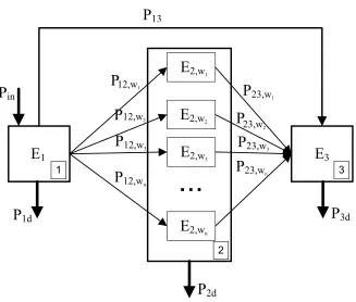
flanking transmission is considered in the SEA model. The energy balance between the subsystems as it is considered

within an SEA approach (see [7]) is illustrated in Fig.2, in which E1,E3 stand for the acoustic energy of the source

room and the receiving room respectively and E2for the vibrational energy of the composite panel. Moreover Pinis

the injected power in the source room, P1d,P2dand P3d stand for the power dissipated by each subsystem and P13is

the non-resonant transmitted power between the rooms.

[Figure 2 about here.]

The derivation of an expression for the total acoustic transmission coefficientτ of the composite structure by merely accounting for its structural dynamic behaviour is summarized in Appendix B (as exhibited in [11]) and reads

τ=

wn X

w=w1 τw+

P13

Pinc

(13)

withτwbeing the transmission coefficient of the wave type w given as

τw=

8ρ2c4πσ2_rad,wnw

ρsω2A(ρsωηw+2ρcσrad,w)

(14)

The non resonant transmission coefficientτnr=P13/Pincfor a diffused acoustic field can be written as in [9]:

τnr(ω)=

1

π(cos2_θ

min−cos2θmax)

Z 2π

0

Z θmax

0

4Z2 0 |iωρs+2Z0|2

σ(θ, φ, ω) cos2θsinθdθdφ (15)

in whichθandφare the incidence angle and the direction angle of the acoustic wave respectively and Z0 =ρc/cosθ

is the acoustic impedance of the medium. The termθmaxstands for the maximum incidence angle, accounting for the

diffuseness of the incident field. It is hereby considered thatθmax=π/2 for all the results presented in the current work.

The termσ(θ, φ, ω) is the corrected radiation efficiency term. It is used in order to account for the finite dimensions of the panel and it is calculated using a spatial windowing correction technique presented in [30].

Eventually the STL of the panel can be expressed as

STL=10 log₁₀ 1

τ

!

(16)

3.2. Parametric sensitivity of the total acoustic transmission

In order to formulate the expression of the Hessian matrix describing the variation of the vibroacoustic

perfor-mance of the structure with respect to its design parameters, the second order derivative ofτ with respect to the

considered set of parameters should be derived and expressed as

∂τ ∂βi

=

wn X

w=w1 ∂τw

∂βi

+∂τnr ∂βi

∂2_τ ∂βj∂βi

=

wn X

w=w1 ∂2_τ

w

∂βj∂βi

+ ∂ 2_τ

nr

∂βj∂βi

(17a)

(17b)

while the sensitivity of the STL index can directly be expressed with regard toτas

∂(S T L)

∂βi

=d(S T L)

dτ ∂τ ∂βi

=− 10 ln(10)τ

∂τ ∂βi

∂2_{(S T L)} ∂βj∂βi

=∂ 2_{(S T L)}

∂τ2 ∂τ ∂βj

∂τ ∂βi

+∂(S T L) ∂τ

∂2_τ ∂βj∂βi

= 10

ln(10)τ2 ∂τ ∂βj

∂τ ∂βi

− 10 ln(10)τ

∂2τ ∂βj∂βi

(18a)

(18b)

In the following sections the evaluation of Eq.17 is discussed.

3.3. Modal density sensitivity

Using Courant’s formula [31], the modal density of each wave type w can be written at a propagation angleφas a

function of the propagating wavenumber and its corresponding group velocity cg:

nw(ω, φ)=

Akw(ω, φ)

2π2_|c

g,w(ω, φ)|

(19)

The angularly averaged modal density of the structure is therefore given as

nw(ω)=

Z π

0

nw(ω, φ) dφ (20)

∂nw(ω, φ)

∂βi

=∂nw(ω, φ) ∂kw(ω, φ)

∂kw(ω, φ)

∂βi

+ ∂nw(ω, φ) ∂cg,w(ω, φ)

∂cg,w(ω, φ)

∂βi

= A

2π2_|c

g,w(ω, φ)|

∂kw(ω, φ)

∂βi

−Akw(ω, φ) sgn(cg,w(ω, φ)) 2π2_|c

g,w(ω, φ)|2

∂cg,w(ω, φ)

∂kw(ω, φ)

∂kw(ω, φ)

∂βi

∂2_n

w(ω, φ)

∂βj∂βi

=∂ 2_n

w(ω, φ)

∂kw(ω, φ)2

∂kw(ω, φ)

∂βj

∂kw(ω, φ)

∂βi

+∂nw(ω, φ) ∂kw(ω, φ)

∂2_k

w(ω, φ)

∂βj∂βi

+ ∂ 2_n

w(ω, φ)

∂cg,w(ω, φ)2

∂cg,w(ω, φ)

∂βj

∂cg,w(ω, φ)

∂βi

+ ∂nw(ω, φ) ∂cg,w(ω, φ)

∂2_c

g,w(ω, φ)

∂βj∂βi

= A

2π2_|c

g,w(ω, φ)|

∂2_k

w(ω, φ)

∂βj∂βi

+Akw(ω, φ) sgn(cg,w(ω, φ)) π2_|c

g,w(ω, φ)|3

∂cg,w(ω, φ)

∂kw(ω, φ)

!2_∂

kw(ω, φ)

∂βj

∂kw(ω, φ)

∂βi

−Akw(ω, φ) sgn(cg,w(ω, φ)) 2π2_|c

g,w(ω, φ)|2

∂2_c

g,w(ω, φ)

∂kw(ω, φ)2

∂kw(ω, φ)

∂βj

∂kw(ω, φ)

∂βi

+∂cg,w(ω, φ) ∂kw(ω, φ)

∂2_k

w(ω, φ)

∂βj∂βi !

(21a)

(21b)

while for the spatially averaged modal density

∂nw(ω)

∂βi

=

Z π

0

∂nw(ω, φ)

∂βi

dφ

∂2_n

w(ω)

∂βj∂βi

=

Z π

0 ∂2_n

w(ω, φ)

∂βj∂βi

dφ

(22a)

(22b)

suggesting that the modal density sensitivity can be expressed merely by

• The sensitivity of the characteristics of the waves travelling within the considered structure with respect to the

structural design (already determined in Sec.2).

• The sensitivity of the modal density with respect to the characteristics of the waves travelling in it.

A similar approach will be followed for computing all the remaining necessary quantities throughout this work. It

should be noted that Eq.21 is derived under the assumption that cg,w(ω, φ),0

3.4. Radiation efficiency sensitivity

In order to avoid the computationally inefficient frequency and directional averaging of the modal dependent radiation efficiency sensitivity ∂σrad,w(ω, φ)

∂βi

, it is practical to employ expressions introducing a direct wavenumber

dependence ofσrad,wsuch as the ones exhibited in [5, 8, 10]. For a generic periodic structure including discontinuities

the assumption of sinusoidal mode shapes is no longer valid, therefore the radiation efficiency should be calculated directly from the PST derived wave mode shapes. The radiation efficiency expression as derived in [10] can therefore be employed. For continuous structures, mode shapes of sinusoidal form can be assumed in order to avoid any FE

discretization errors in the solution. The set of asymptotic formulas given in [8] can be used for computing the

σrad,w(k (ω))=               

1

p

1−µ2 µ <1

Lx+Ly

πµκLxLy p

µ2₋₁ ln µ+1

µ−1

!

+ 2µ µ2₋₁

!

µ >1

withµ=

      

k2_x+k_y2

κ2

      

1/2

, whereκ=ω/c is the acoustic wavenumber. It is noted that the above expressions are largely

overestimating the radiation efficiency of the structure close to the coincidence frequency. An efficient approximation ofσrad,wwhen k=κis given in [8] as

σrad,w(k (ω))=

0.5−0.15 min (Lx,Ly)/max (Lx,Ly)

q

k min (Lx,Ly)

Three domains will therefore be distinguished for the radiation efficiency of the panel. It has been empirically observed that the above cited relations overestimate the radiation efficiency of the panel within a region 0.90< µ <

1.05. The following relations forσrad,w(k (ω)) are therefore hereby suggested

σrad,w=

1

p

1−µ2 µ <0.90 σrad,w=

Lx+Ly

πµκLxLy p

µ2₋₁ ln µ+1

µ−1

!

+ 2µ µ2₋₁

!

µ >1.05

σrad,w=

0.5−0.15 min (Lx,Ly)/max (Lx,Ly)

q

k min (Lx,Ly) µ=1

(23a)

(23b)

(23c)

In the region 0.90< µ <1.05 a shape preserving Hermite interpolation function is employed assuring the continuity

and double differentiability for the entire spectrum of theσrad,wexpression. The sensitivity expressions can therefore

∂σrad,w

∂βi

=∂σrad,w ∂kw

∂kw

∂βi

= kw

κ2_(1−k2

w/κ2)3/2

∂kw

∂βi

µ <0.90

∂2σrad,w

∂βj∂βi

=∂ 2_σ

rad,w

∂k2

w

∂kw

∂βj

∂kw

∂βi

+∂σrad,w ∂kw

∂2_k

w

∂βj∂βi

= 1

κ2_(1−k2

w/κ2)3/2

+ 3k

2

w

κ4_(1−k2

w/κ2)5/2

!_∂

kw

∂βj

∂kw

∂βi

+ kw

κ2_(1−k2

w/κ2)3/2

∂2_k

w

∂βj∂βi

µ <0.90

∂σrad,w

∂βi

=− 4kw(Lx+Ly) πLxLyκ3((k2w−κ2)/κ2)5/2

∂kw

∂βi

−

kw(Lx+Ly) ln

µ+1

µ−1+(2κ

2_µ)/(k2

w−κ

2₎

!

πLxLyκ3((k2w−κ2)/κ2)1/2(k2w/κ2)3/2

∂kw

∂βi

−

kw(Lx+Ly) ln

µ+1

µ−1+(2κ

2_µ)/(k2

w−κ

2₎

!

πLxLyκ3((k2w−κ2)/κ2)3/2µ

∂kw

∂βi

µ >1.05

∂2_σ

rad,w

∂βj∂βi

=

k2

w(Lx+Ly)(4κ6µ+6k6wln

µ+1

µ−1−2κ

6_lnµ+1 µ−1 −10k

2

wκ

4_µ)

πLxLyκ11((k2w−κ2)/κ2)7/2(k2w/κ2)5/2

∂kw

∂βj

∂kw

∂βi

+

k2

w(Lx+Ly)(36kw4κ2µ+7k2wκ4ln

µ+1

µ−1−11k

4

wκ

2_lnµ+1 µ−1)

πLxLyκ11((kw2−κ2)/κ2)7/2(kw2/κ2)5/2

∂kw

∂βj

∂kw

∂βi

− 4kw(Lx+Ly) πLxLyκ3((kw2−κ2)/κ2)5/2

∂2kw

∂βj∂βi

−

kw(Lx+Ly) ln

µ+1

µ−1+(2κ

2_µ)/(k2

w−κ

2₎

!

πLxLyκ3((k2w−κ2)/κ2)1/2(k2w/κ2)3/2

∂2kw

∂βj∂βi

−

kw(Lx+Ly) ln

µ+1

µ−1+(2κ

2_µ)/(k2

w−κ2) !

πLxLyκ3((k2w−κ2)/κ2)3/2µ

∂2_k

w

∂βj∂βi

µ >1.05

(24a)

(24b)

(24c)

(24d)

while the interpolation function is used for expressing the sensitivity ofσrad,wfor the remaining spectrum.

3.5. Damping loss factor sensitivity

Reducing the acoustic transparency of a structural panel by increasing its intrinsic damping properties is a popular

noise reduction strategy within the modern industry and oftentimes an effective option, particularly in the high fre-quency range. It is therefore particularly useful to develop dedicated models for evaluating the effect of the increase of the damping coefficientγof the material comprised in a single layer of the composite structure on its total loss factor. Having a look at the form of the eigenvalue problem in Eq.6 it can be deduced that expressing the total loss

factor of the structural panel as a function of the real and imaginary parts of the resulting eigenvalues (as in [32, 33])

can be particularly practical.

ηw(ω, φ)=2

ωiωr

ω2

r−ω2i

(25)

withηn(ω, φ) the loss factor for the wave type w at a certain angular frequencyωand propagating towards a certain

directionφ. The total frequency dependent loss factor of a certain wavetype can be computed as

ηw(ω)=

Rπ

0 ηn(ω, φ)dφ

π (26)

which can be evaluated at the entire spectrum of interest. The sensitivity of the directional loss factorηw(ω, φ) can

therefore be expressed as

∂ηw(ω, φ)

∂βi

= ∂ηw(ω, φ) ∂ωr(ω, φ)

∂ωr(ω, φ)

∂βi

+∂ηw(ω, φ) ∂ωi(ω, φ)

∂ωi(ω, φ)

∂βi =−      

2ωi

ω2_i −ω2

r

+ 4ωiω 2

r

(ω2_i −ω2

r)2      

∂ωr(ω, φ)

∂βi +      

4ω2_iωr

(ω2_i −ω2

r)2

− 2ωr ω2_i −ω2

r      

∂ωi(ω, φ)

∂βi

∂2_η

w(ω, φ)

∂βj∂βi

= ∂ 2_η

w(ω, φ)

∂ωr(ω, φ)2

∂ωr(ω, φ)

∂βj

∂ωr(ω, φ)

∂βi

+∂ηw(ω, φ) ∂ωr(ω, φ)

∂2_ω

r(ω, φ)

∂βj∂βi

+∂ 2_η

w(ω, φ)

∂ωi(ω, φ)2

∂ωi(ω, φ)

∂βj

∂ωi(ω, φ)

∂βi

+∂ηw(ω, φ) ∂ωi(ω, φ)

∂2_ω

i(ω, φ)

∂βj∂βi

=−      

16ωiω3r

(ω2

i −ω

2

r)3

+ 12ωiωr

(ω2

i −ω

2

r)2      

∂ωr(ω, φ)

∂βj

∂ωr(ω, φ)

∂βi −      

2ωi

ω2

i −ω

2

r

+ 4ωiω 2

r

(ω2

i −ω

2

r)2      

∂2_ω

r(ω, φ)

∂βj∂βi

+      

12ωiωr

(ω2

i −ω2r)2

− 16ω 3

iωr

(ω2

i −ω2r)3      

∂ωi(ω, φ)

∂βj

∂ωi(ω, φ)

∂βi +      

4ω2

iωr

(ω2

i −ω2r)2

− 2ωr ω2

i −ω2r      

∂2_ω

i(ω, φ)

∂βj∂βi

(27a)

(27b)

while for the total loss factor of the panel

∂ηw(ω)

∂βi = Z π 0 1 π

∂ηw(ω, φ)

∂βi

dφ

∂2ηw(ω)

∂βj∂βi

=

Z π

0

1

π

∂2ηw(ω, φ)

∂βj∂βi

dφ

(28a)

(28b)

to be evaluated in the frequency bands of interest.

3.6. Sensitivity of the resonant acoustic transmission

∂τw

∂βi

= ∂τw ∂σrad,w

∂σrad,w

∂βi

+∂τw ∂nw

∂nw

∂βi

+∂τw ∂ηw

∂ηw

∂βi

+∂τw ∂ρs

∂ρs

∂βi

∂2τw

∂βj∂βi

= ∂ 2_τ

w

∂σ2

rad,w

∂σrad,w

∂βj

∂σrad,w

∂βi

+ ∂τw ∂σrad,w

∂2_σ

rad,w

∂βj∂βi

+∂ 2_τ

w

∂n2

w

∂nw

∂βj

∂nw

∂βi

+∂τw ∂nw

∂2_n

w

∂βj∂βi

+∂ 2_τ w ∂η2 w ∂ηw ∂βj ∂ηw ∂βi

+∂τw ∂ηw

∂2_η

w

∂βj∂βi

+∂ 2_τ w ∂ρ2 s ∂ρs ∂βj ∂ρs ∂βi

+∂τw ∂ρs

∂2_ρ

s

∂βj∂βi

(29a)

(29b)

with the transmission coefficient related sensitivity terms being expressed as

∂τw

∂σrad,w

= 16πc 4_n

wρ2σrad,w Aω2_ρ

s(ηwωρs+2cρσrad,w)

− 16πc 5_n

wρ3σ2_rad,w Aω2_ρ

s(ηwωρs+2cρσrad,w)2

∂2_τ

w

∂σ2

rad,w

= 16πc

4_n

wρ2 Aω2_ρ

s(ηwωρs+2cρσrad,w)

− 64πc 5_n

wρ3σrad,w Aω2_ρ

s(ηwωρs+2cρσrad,w)2

+ 64πc 6_n

wρ4σ2_rad,w Aω2_ρ

s(ηwωρs+2cρσrad,w)3

∂τw

∂nw

=

8πc4_ρ2_σ2

rad,w Aω2_ρ

s(ηwωρs+2cρσrad,w)

∂2_τ

w

∂n2

w

=0

∂τw

∂ηw

=− 8πc 4_n

wρ2σ2_rad,w Aω(ηwωρs+2cρσrad,w)2

∂2τw

∂η2

w

= 16πc 4_n

wρ2ρsσ2_rad,w

(Aηwωρs+2cρσrad,w)3

∂τw

∂ρs

=− 8πc 4_n

wρ2σ2_rad,w Aω2_ρ2

s(ηwωρs+2cρσrad,w)

− 8πc 4_η

wnwρ2σ2_rad,w Aωρs(ηwωρs+2cρσrad,w)2

∂2_τ

w

∂ρ2

s

= 16

πc4η2

wnwρ2σ2_rad,w Aρs(ηwωρs+2cρσrad,w)3

+ 16

πc4nwρ2σ2_rad,w Aω2_ρ3

s(ηwωρs+2cρσrad,w)

+ 16

πc4ηwnwρ2σ2_rad,w Aωρ2

s(ηwωρs+2cρσrad,w)2

(30a) (30b) (30c) (30d) (30e) (30f) (30g) (30h)

All the necessary quantities have by now been computed from the considerations introduced above and the

reso-nant acoustic transmission sensitivity can thus be evaluated in Eq.29.

3.7. Sensitivity of the nonresonant acoustic transmission

Nonresonant acoustic transmission is induced by the structural/acoustic coupling of mass controlled (low fre-quency) and stiffness controlled (high frequency) modes having a resonance frequency outside the considered band. Mass controlled modes can actually induce a significant amount of acoustic transmission and are considered within

the analysis through Eq.15. It is evident thatτnr(ω) as expressed in Eq.15 is insensitive to all structural design

affect the nonresonant term are the layer thicknesses and densities of the composite structure. The parametric design sensitivities can therefore be written as

∂τnr(ω)

∂βi

= 1

π(cos2_θ

min−cos2θmax)

Z 2π

0

Z θmax

0

∂τnr(θ, φ, ω)

∂βi

dθdφ (31)

with the sensitivity of the directional transmission coefficient expressed as

∂τnr(θ, φ, ω)

∂βi

= ∂τnr(θ, φ, ω) ∂ρs

∂ρs

∂βi

=−8Z 2

0ωσ(θ, φ, ω) cos 2_θsinθi |2Z0+ρsωi|3

∂ρs

∂βi

(32)

While for the second order sensitivity we have

∂2_τ

nr(ω)

∂βj∂βi

= 1

π(cos2_θ

min−cos2θmax)

Z 2π

0

Z θmax

0 ∂2_τ

nr(θ, φ, ω)

∂ρ2

s

∂ρs

∂βj

∂ρs

∂βi

+∂τnr(θ, φ, ω) ∂ρs

∂2_ρ

s

∂βj∂βi

dθdφ (33)

with

∂2_τ

nr(θ, φ, ω)

∂ρ2

s

=−24Z 2 0ω

2_{σ(θ, φ, ω) cos}2_θsinθ |2Z0+ρsωi|4

(34)

The computational cost of Eqs.31,33 is significantly reduced by the fact that the geometric radiation efficiency termσ(θ, φ, ω) is solely dependent on the area A of the considered structure which is not under investigation and is

therefore computed only once in the optimization process. The quantity| 2Z0+ρsωi |is therefore the only one that

needs being recomputed for every design alteration. Given thatρs = lmax X

l=l1

ρm,lhl withρm,l the mass density of layer l

and hlits thickness, it is straightforward to derive the quantities

∂ρs

∂βi

∂ρs

∂βj

and ∂

2_ρ

s

∂βi∂βj

for the composite panel.

4. Formulation of the optimization problem

The Newton’s method will be hereby employed (ensuring quadratic convergence towards the solution) in order to

optimise the considered set of parameters, which in the general orthotropic multilayer case can be expressed as

p=

Ex,1Ey,1Ez,1vxy,1vxz,1vyz,1Gxy,1Gxz,1Gyz,1h1ρm,1· · ·ρm,lmax

⊤

(35)

with lmaxthe maximum number of layers. It is interesting to note that includingηin an optimization procedure will

not provide any helpful information, asδηwill not directly affect neither the mass, nor the stiffness of the panel. On the other hand it will always be beneficial for the reduction ofτw, which suggests that a maximumηwill always be

the result of the computation. An effective way of including damping in the optimization process would be explicitly relating the increase of damping coefficientγlfor layer l with the mass of the layer (e.g. accounting for the mass and

damping increase implied by viscoleastic material inclusions).

The parameters may be considered to be constrained (e.g. βi∈[βi,min, βi,max]). The objective functionF(p) to be

loss should be included inF(p) (if not maximising the mass of the panel would be the evident solution for minimising

the acoustic transmission). There is a number of cost criteria that can be applied to the stress-strain matrix coefficients [34] of a laminate in order to account for its axial, shear and flexural stiffness. A number of manufacturing related constraints (accounting for the realizability of the computed optimal design) can also be added to the optimization

problem.

The cost function can eventually be expressed as

F(p)=ξ3τ3(p)+ξ2τ2(p)+ξ1τ(p)+ξ0+δ3ρ3_s(p)+δ2ρ2_s(p)+δ1ρs(p)+δ0+ζ3d3s(p)+ζ2d

2

s(p)+ζ1ds(p)+ζ0 (36)

withτ,ρsand dsbeing the acoustic, mass and stiffness performance indices respectively andξi,δi,ζicoefficients that

allow the designer to apply a polynomial curve fitting to the available cost data; thus facilitating the differentiability of F(p). Higher order polynomial or exponential fitting functions may be applied without loss of accuracy. The gradient

vector ofF(p) can therefore be computed as

∇F(p)=

( _∂F(p)

∂Ex,1 ∂F(p)

∂Ey,1 ∂F(p)

∂Ez,1 ∂F(p)

∂vxy,1 ∂F(p)

∂vxz,1 ∂F(p)

∂vyz,1 ∂F(p)

∂Gxy,1 ∂F(p)

∂Gxz,1 ∂F(p)

∂Gyz,1 ∂F(p)

∂h1

∂F(p)

∂ρm,1

· · · ∂F(p) ∂ρm,lmax

)⊤

(37)

The derivatives ofF(p) can be calculated using the chain rule (e.g. ∂(ξ3τ

3₎ ∂βi

=3ξ3τ2∂τ ∂βi

and∂

2_(ξ3τ3₎ ∂βj∂βi

=6ξ3τ∂τ ∂βj

∂τ ∂βi

+

3ξ3τ2 ∂ 2_τ ∂βj∂βi

). The Hessian matrix is subsequently formed using the computed second order sensitivity values

H=∇2_F

(p)=                                                                                                                                                 ∂2 F(p)

∂E2 x,1

∂2 F(p)

∂Ex,1∂Ey,1

∂2 F(p)

∂Ex,1∂Ez,1

∂2 F(p)

∂Ex,1∂vxy,1

∂2 F(p)

∂Ex,1∂vxz,1

∂2 F(p)

∂Ex,1∂vyz,1

∂2 F(p)

∂Ex,1∂Gxy,1

∂2 F(p)

∂Ex,1∂Gxz,1

∂2 F(p)

∂Ex,1∂Gyz,1

∂2 F(p)

∂Ex,1∂h1

∂2 F(p)

∂Ex,1∂ρm,1 · · · ∂

2 F(p)

∂Ex,1∂ρm,lmax ∂2_F(p)

∂Ey,1∂Ex,1

∂2_F(p)

∂E2 y,1

∂2_F(p)

∂Ey,1∂Ez,1

∂2_F(p)

∂Ey,1∂vxy,1

∂2_F(p)

∂Ey,1∂vxz,1

∂2_F(p)

∂Ey,1∂vyz,1

∂2_F(p)

∂Ey,1∂Gxy,1

∂2_F(p)

∂Ey,1∂Gxz,1

∂2_F(p)

∂Ey,1∂Gyz,1

∂2_F(p)

∂Ey,1∂h1

∂2_F(p)

∂Ey,1∂ρm,1 · · · ∂

2_F(p)

∂Ey,1∂ρm,lmax ∂2_F(p)

∂Ez,1∂Ex,1

∂2_F(p)

∂Ez,1∂Ey,1

∂2_F(p)

∂E2 z,1

∂2_F(p)

∂Ez,1∂vxy,1

∂2_F(p)

∂Ez,1∂vxz,1

∂2_F(p)

∂Ez,1∂vyz,1

∂2_F(p)

∂Ez,1∂Gxy,1

∂2_F(p)

∂Ez,1∂Gxz,1

∂2_F(p)

∂Ez,1∂Gyz,1

∂2_F(p)

∂Ez,1∂h1

∂2_F(p)

∂Ez,1∂ρm,1 · · · ∂

2_F(p)

∂Ez,1∂ρm,lmax ∂2_F(p)

∂vxy,1∂Ex,1

∂2_F(p)

∂vxy,1∂Ey,1

∂2_F(p)

∂vxy,1∂Ez,1

∂2_F(p)

∂v2 xy,1

∂2_F(p)

∂vxy,1∂vxz,1

∂2_F(p)

∂vxy,1∂vyz,1

∂2_F(p)

∂vxy,1∂Gxy,1

∂2_F(p)

∂vxy,1∂Gxz,1

∂2_F(p)

∂vxy,1∂Gyz,1

∂2_F(p)

∂vxy,1∂h1

∂2_F(p)

∂vxy,1∂ρm,1 · · · ∂

2_F(p)

∂vxy,1∂ρm,lmax ∂2

F(p)

∂vxz,1∂Ex,1

∂2 F(p)

∂vxz,1∂Ey,1

∂2 F(p)

∂vxz,1∂Ez,1

∂2 F(p)

∂vxz,1∂vxy,1

∂2 F(p)

∂v2 xz,1

∂2 F(p)

∂vxz,1∂vyz,1

∂2 F(p)

∂vxz,1∂Gxy,1

∂2 F(p)

∂vxz,1∂Gxz,1

∂2 F(p)

∂vxz,1∂Gyz,1

∂2 F(p)

∂vxz,1∂h1

∂2 F(p)

∂vxz,1∂ρm,1 · · · ∂

2 F(p)

∂vxz,1∂ρm,lmax ∂2_F(p)

∂vyz,1∂Ex,1

∂2_F(p)

∂vyz,1∂Ey,1

∂2_F(p)

∂vyz,1∂Ez,1

∂2_F(p)

∂vyz,1∂vxy,1

∂2_F(p)

∂vyz,1∂vxz,1

∂2_F(p)

∂v2 yz,1

∂2_F(p)

∂vyz,1∂Gxy,1

∂2_F(p)

∂vyz,1∂Gxz,1

∂2_F(p)

∂vyz,1∂Gyz,1

∂2_F(p)

∂vyz,1∂h1

∂2_F(p)

∂vyz,1∂ρm,1 · · · ∂

2_F(p)

∂vyz,1∂ρm,lmax ∂2_F(p)

∂Gxy,1∂Ex,1

∂2_F(p)

∂Gxy,1∂Ey,1

∂2_F(p)

∂Gxy,1∂Ez,1

∂2_F(p)

∂Gxy,1∂vxy,1

∂2_F(p)

∂Gxy,1∂vxz,1

∂2_F(p)

∂Gxy,1∂vyz,1

∂2_F(p)

∂G2 xy,1

∂2_F(p)

∂Gxy,1∂Gxz,1

∂2_F(p)

∂Gxy,1∂Gyz,1

∂2_F(p)

∂Gxy,1∂h1

∂2_F(p)

∂Gxy,1∂ρm,1 · · · ∂

2_F(p)

∂Gxy,1∂ρm,lmax ∂2_F(p)

∂Gxz,1∂Ex,1

∂2_F(p)

∂Gxz,1∂Ey,1

∂2_F(p)

∂Gxz,1∂Ez,1

∂2_F(p)

∂Gxz,1∂vxy,1

∂2_F(p)

∂Gxz,1∂vxz,1

∂2_F(p)

∂Gxz,1∂vyz,1

∂2_F(p)

∂Gxz,1∂Gxy,1

∂2_F(p)

∂G2 xz,1

∂2_F(p)

∂Gxz,1∂Gyz,1

∂2_F(p)

∂Gxz,1∂h1

∂2_F(p)

∂Gxz,1∂ρm,1 · · · ∂

2_F(p)

∂Gxz,1∂ρm,lmax ∂2_F(p)

∂Gyz,1∂Ex,1

∂2_F(p)

∂Gyz,1∂Ey,1

∂2_F(p)

∂Gyz,1∂Ez,1

∂2_F(p)

∂Gyz,1∂vxy,1

∂2_F(p)

∂Gyz,1∂vxz,1

∂2_F(p)

∂Gyz,1∂vyz,1

∂2_F(p)

∂Gyz,1∂Gxy,1

∂2_F(p)

∂Gyz,1∂Gxz,1

∂2_F(p)

∂G2 yz,1

∂2_F(p)

∂Gyz,1∂h1

∂2_F(p)

∂Gyz,1∂ρm,1 · · · ∂

2_F(p)

∂Gyz,1∂ρm,lmax ∂2_F(p)

∂h1∂Ex,1

∂2_F(p)

∂h1∂Ey,1

∂2_F(p)

∂h1∂Ez,1

∂2_F(p)

∂h1∂vxy,1

∂2_F(p)

∂h1∂vxz,1

∂2_F(p)

∂h1∂vyz,1

∂2_F(p)

∂h1∂Gxy,1

∂2_F(p)

∂h1∂Gxz,1

∂2_F(p)

∂h1∂Gyz,1

∂2_F(p)

∂h2 1

∂2_F(p)

∂h1∂ρm,1

· · · ∂ 2_F(p)

∂h1∂ρm,lmax ∂2_F

(p)

∂ρm,1∂Ex,1

∂2_F

(p)

∂ρm,1∂Ey,1

∂2_F

(p)

∂ρm,1∂Ez,1

∂2_F

(p)

∂ρm,1∂vxy,1

∂2_F

(p)

∂ρm,1∂vxz,1

∂2_F

(p)

∂ρm,1∂vyz,1

∂2_F

(p)

∂ρm,1∂Gxy,1

∂2_F

(p)

∂ρm,1∂Gxz,1

∂2_F

(p)

∂ρm,1∂Gyz,1

∂2_F

(p)

∂ρm,1∂h1

∂2_F

(p)

∂ρ2 m,1

· · · ∂ 2_F

(p)

∂ρm,1∂ρm,lmax

· · · ·

∂2_F(p)

∂ρm,lmax∂Ex,1

∂2_F(p)

∂ρm,lmax∂Ey,1

∂2_F(p)

∂ρm,lmax∂Ez,1

∂2_F(p)

∂ρm,lmax∂vxy,1

∂2_F(p)

∂ρm,lmax∂vxz,1

∂2_F(p)

∂ρm,lmax∂vyz,1

∂2_F(p)

∂ρm,lmax∂Gxy,1

∂2_F(p)

∂ρm,lmax∂Gxz,1

∂2_F(p)

∂ρm,lmax∂Gyz,1

∂2_F(p)

∂ρm,lmax∂h1

∂2_F(p)

∂ρm,lmax∂ρm,1

· · · ∂ 2_F(p)

∂ρ2 m,lmax

                                                                                                                                                (38)

A commercially embedded constrained nonlinear optimization algorithm [35] is eventually employed in order to

5. Numerical case studies

In order to validate the exhibited optimization approach, an asymmetric sandwich panel comprising two facesheets

and a core is modelled in this section. The lower facesheet has a thickness h1=1mm and is made of a material having

ρm,1=3000e−9kg/mm3, E1 = 70GPa and a Poisson’s ration v1=0.1. The upper facesheet has a thickness equal to

h3=2mm and is made of the same material as the lower facesheet. The core has a thickness h2=10mm and is made of a material withρm,2=50e−9kg/mm3, E2 =0.07GPa and v2=0.4. Three FEs are used in the sense of thickness in order

to model the structure. All computations were conducted using the R2013a version of MATLABr_.

5.1. Results on the wave sensitivity analysis of a layered structure

In this section the sensitivity of the wave characteristics with respect to the mechanical and geometric

characteris-tics of the sandwich panel are sought as discussed in Sec.2. The results are compared to a FD approach throughout this

section. In order to implement the FD approach a perturbation of 0.1% was considered for each structural parameter.

The resulting FD sensitivity can be computed by

∂k

∂β =

kp−k0 βp−β0

(39)

with kpthe perturbed wavenumber value forβpand k0the corresponding wavenumber for the unperturbed parameter β0.

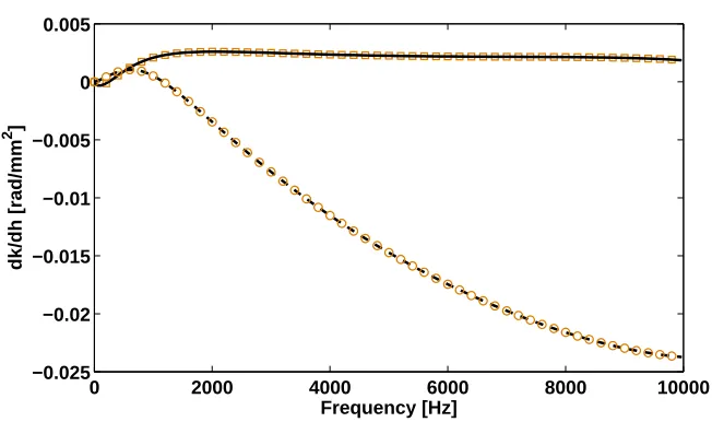
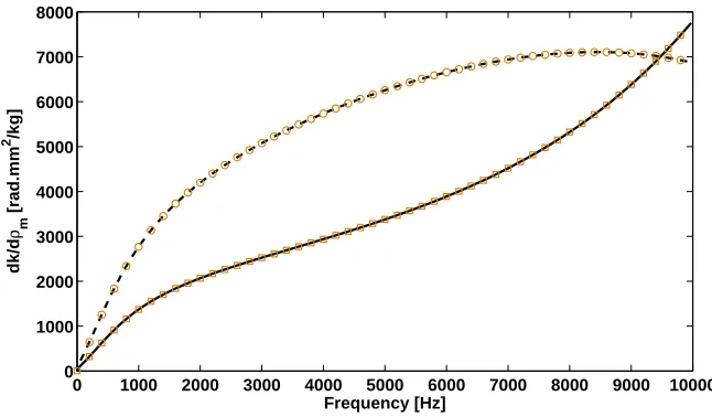
The sensitivity of the flexural wavenumber k with respect to the thickness of each facesheet layer is presented

in Fig.3. It is particularly interesting to note that in the very low frequency range increasing the thickness of both

facesheets will imply a softening effect to the structural behaviour, shifting the flexural wavenumbers upwards. This mainly suggests that the effect of the added mass overcomes the effect of added stiffness for bothδh1andδh3. However

at higher frequencies the results change radically for the thicker upper facesheet, withδh3now shifting the

wavenum-bers to lower values, suggesting a stiffening phenomenon in the structural dynamic behaviour. An excellent agreement is observed between the presented approach and the FD method.

[Figure 3 about here.]

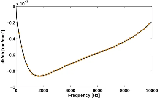
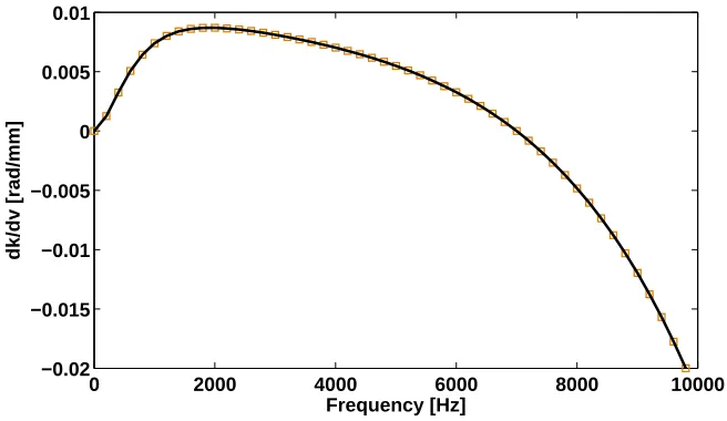
The sensitivity of k with respect to the thickness of the sandwich core layer is presented in Fig.4. A very

in-teresting effect is that the influence ofδh2 on the flexural wavenumber becomes maximum for a certain frequency

(approximately 2000 Hz), where the stiffening effect ofδh2becomes maximum. An intense nonlinearity is observed

in the relation ofδωtoδk. A constant decrease of this influence is observed beyond that point. The stiffening effect is probably due to the greater separation of the two facesheets withδh2. It is very probable however that for higher

wavenumber valuesδhcwill have a softening effect on the flexural wavenumber with the depicted curve passing to

positive values okδk. This is the frequency range within which the two facesheets of the structure start vibrating

[Figure 4 about here.]

In Fig.5, the sensitivity of k with respect to the mass density of the sandwich facesheet layers is presented. As

expected, bothδρm,1andδρm,3will shift the wavenumber curve to higher values, suggesting a softening phenomenon.

This effect will be greater for the thicker upper facesheet at low k values. A highly nonlinear behaviour is again observed and it is interesting to see that there is a critical frequency value at which the effect ofδρm,1andδρm,3will

be the same. Beyond this critical wavenumber the softening effect will paradoxically be more intense forδρm,1.

[Figure 5 about here.]

The perturbation of k with respect to v2for the sandwich core is presented in Fig.6. The effect ofδv2is softening

up to a certain wavenumber value, beyond which an intense decrease of the sensitivity is observed which stiffens the flexural structural behaviour.

[Figure 6 about here.]

5.2. Results on the SEA sensitivity analysis of a layered structure

In this section the sensitivity of the SEA quantities, namely the modal density, the radiation efficiency and the damping loss factor are computed as discussed in Sec.3 and evaluated.

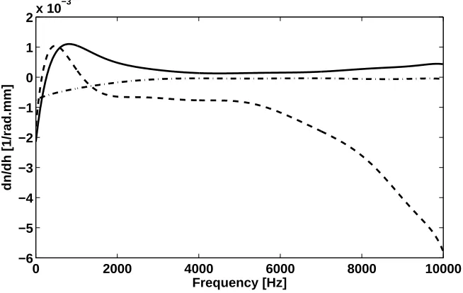
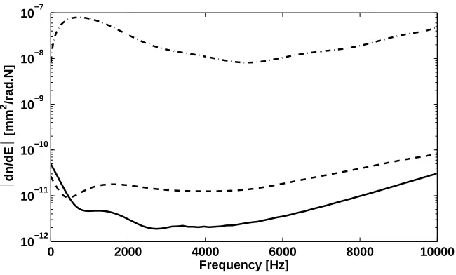
The first order sensitivity of the modal density of the composite panel with regard to the layer thicknesses and

Young’s moduli are exhibited in Figs.7,8 respectively. In Fig.8 all sensitivity values are negative, it was thus preferred

to present the absolute result values in order to employ a clearer logarithmic scale. It can be observed that the

stiffening effect induced byδh3in the high frequency range, also induces a high reduction of the modal density, while

a maximum softening effect is observed for bothδh1,δh3in the low frequency range (approximately 1000 Hz). With

regard to the effect of the Young’s modulus it is observed that its increase can imply more drastic hardening effects for the core layer compared to the one of the facesheets.

[Figure 7 about here.]

[Figure 8 about here.]

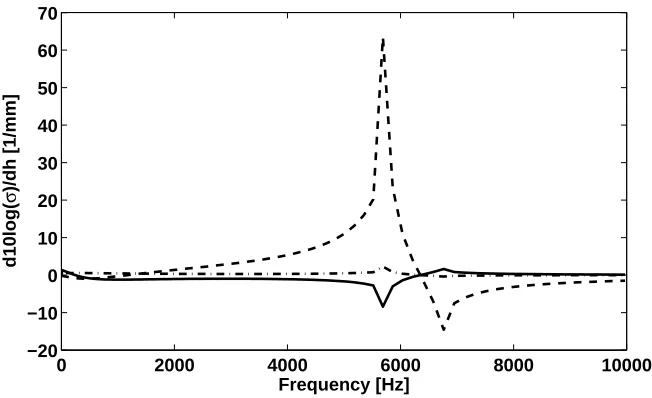
The sensitivity of the acoustic radiation efficiency for the composite panel with regard to the layer thicknesses is presented in Fig.9. In order to use a clearer logarithmic scale the quantityδ10log(σ)/δh is plotted. It is generally observed that altering the thickness of the thicker facesheet h3will have a maximum effect on the radiation efficiency,

while the opposite is true for altering the thickness of the core layer. The maximum impact onσ is as expected

observed around the acoustic coincidence frequency (approximately 5800 Hz in this case study). It is interesting to

note that the effect ofδh1will have an opposite effect onσcompared toδh3.

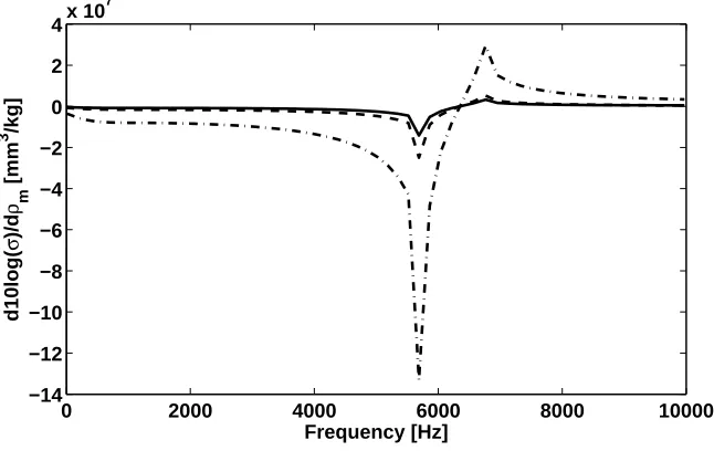
The same quantity is presented in Fig.10, this time as a function of the mass densities of the three layers. This

time the effect ofδρm,2 will have a maximum impact on the acoustic radiation efficiency (probably due to the higher

[Figure 9 about here.]

[Figure 10 about here.]

The sensitivity of the loss factorηfor the flexural wave is subsequently discussed. Its first order sensitivity with

regard to the layer thicknesses is exhibited in Fig.11. It is evident that the maximum impact ofδhion the total loss

factor of the panel takes place in the low frequency range. For higher frequencies it can be observed thatδη/δh1

converges to a constant value, while the increase of the core thickness has a continuously diminishing impact onη.

In Fig.12 the same quantity is presented, this time as a function of the individual damping coefficient of each layer

γi. Throughout the entire frequency range it is observed that increasing the damping coefficient of the core layerδγ2

will have a maximum effect on the total loss factor of the panel. It is observed that the effect ofδγion the total loss

factor is diminishing with frequency.

[Figure 11 about here.]

[Figure 12 about here.]

The impact of the structural parameters on the acoustic transmission coefficient and the STL of the composite structure is eventually computed. In Fig.13 the sensitivity of the structure’s TL with regard to the layer thicknesses

is presented. It is evident that altering the thickness of the upper thicker layer will induce the maximum effect on TL, especially close to the acoustic coincidence region. On the other hand, altering the core thickness will have an

insignificant effect on the TL index.

[Figure 13 about here.]

In Fig.14 the sensitivity of the TL with regard to the layer mass densities is presented. It is evident that the results

follow the trend of the ones shown for the radiation efficiency of the panel in Fig.10 with the mass density of the core layer being the one that influences the TL the most.

[Figure 14 about here.]

The same result is exhibited in Fig.15, this time regarding the sensitivity with respect to the Young’s moduli of the

layers. Once again it is observed that altering the Young’s modulus of the core can have the most significant impact,

while the influence ofδE1andδE3are generally insignificant.