Swimming mechanics and behavior of the shallow water brief squid Lolliguncula brevis

Resistive and propulsive forces associated with jet propulsion have been investigated in scallops (Trueman, 1975; Vogel, 1985; Dadswell and Weihs, 1990; Millward and Whyte, 1992; Cheng and DeMont, 1996; Cheng et al., 1996), jellyfish (Daniel, 1983; Daniel, 1985; DeMont and Gosline, 1988), salps (Madin, 1990) and frogfishes (Fish, 1987). The best-known jetters are cephalopods, including the chambered Nautilus, octopuses, cuttlefishes and squid. Much of the hydrodynamic work on cephalopods has been performed on Nautilus and centers around the effects of the shell on surrounding flow, locomotion and mode of life (Raup, 1967; Chamberlain and Westerman, 1976; Chamberlain, 1976; Chamberlain, 1980; Chamberlain, 1981; Chamberlain, 1990; Holland, 1987; O’Dor et al., 1990). Although there are a number of papers examining swimming energetics of squid (O’Dor, 1982; Webber and O’Dor, 1985; Webber and O’Dor, 1986; O’Dor and Webber, 1986; O’Dor and Webber, 1991; O’Dor et al., 1994; Finke et al., 1996), only Johnson et al. (Johnson et al., 1972), O’Dor (O’Dor, 1988) and Anderson and

DeMont (Anderson and DeMont, 2000) focus on the hydrodynamics and mechanics of squid locomotion. Johnson et al. (Johnson et al., 1972) outline a theoretical approach to squid swimming, but it has limited applicability since it is based on one contraction of the mantle musculature and incorporates a number of oversimplifications and assumptions. O’Dor (O’Dor, 1988) provides a more in-depth and informative examination of the forces acting on adult squid Loligo opalescens (and to a lesser extent Illex illecebrosus) using video analysis and recordings of mantle cavity pressure. Anderson and DeMont (Anderson and DeMont, 2000) provide interesting information on propulsive efficiency and some unsteady hydrodynamics of adult Loligo pealei.

The limited research on squid swimming mechanics is surprising given the versatility of squid as swimmers. Squid may hover in one spot, change direction rapidly with apparent ease, stop and reverse direction and ascend and descend almost vertically. Squid are capable of such impressive maneuvers because of interactions between three systems: (i) the jet,

3655

Printed in Great Britain © The Company of Biologists Limited 2001 JEB3819

Although squid are among the most versatile swimmers and rely on a unique locomotor system, little is known about the swimming mechanics and behavior of most squid, especially those that swim at low speeds in inshore waters. Shallow-water brief squid Lolliguncula brevis, ranging in size from 1.8 to 8.9 cm in dorsal mantle length (DML), were placed in flumes and videotaped, and the data were analyzed using motion-analysis equipment. Flow visualization and force measurement experiments were also performed in water tunnels. Mean critical swimming speeds (Ucrit) ranged from 15.3 to 22.8 cm s−1,

and mean transition speeds (Ut; the speed above which

squid swim exclusively in a tail-first orientation) varied from 9.0 to 15.3 cm s−1_{. At low speeds, negatively buoyant}

brief squid generated lift and/or improved stability by positioning the mantle and arms at high angles of attack, directing high-speed jets downwards (angles >50 °) and using fin activity. To reduce drag at high speeds, the squid

decreased angles of attack and swam tail-first. Fin motion, which could not be characterized exclusively as drag- or lift-based propulsion, was used over 50–95 % of the sustained speed range and provided as much as 83.8 % of the vertical and 55.1 % of the horizontal thrust. Small squid (<3.0 cm DML) used different swimming strategies from those of larger squid, possibly to maximize thrust benefits from vortex ring formation. Furthermore, brief squid employed various unsteady behaviors, such as manipulating funnel diameter during jetting, altering arm position and swimming in different orientations, to boost swimming performance. These results demonstrate that locomotion in slow-swimming squid is complex, involving intricate spatial and temporal interactions between the mantle, fins, arms and funnel.

Key words: squid, negative buoyancy, hydrodynamics, swimming, jet propulsion, Lolliguncula brevis, fin.

Summary

Introduction

Swimming mechanics and behavior of the shallow-water brief squid

Lolliguncula brevis

Ian K. Bartol

*, Mark R. Patterson

and Roger Mann

1_{Department of Organismic Biology, Ecology, and Evolution, 621 Charles E. Young Drive South, University of}

California, Los Angeles, CA 90095-1606, USA and 2School of Marine Science, Virginia Institute of Marine Science, College of William and Mary, Gloucester Point, VA 23062-1346, USA

which may be directed using a funnel maneuverable within a hemisphere below the body, (ii) the fins, which may undulate and/or flap independently or synchronously, and (iii) the arms, which may be positioned at different angles of attack, moved vertically and laterally and extended and retracted to maximize and minimize surface area.

Although O’Dor (O’Dor, 1988) and Anderson and DeMont (Anderson and DeMont, 2000) provide important information on moderately large squid species, which swim at moderate to high speeds and rely heavily on the jet for propulsion, several important areas of locomotion in squid remain unexplored. (i) Little is known about how swimming mechanics change with size in squid. With the exception of some general observations on Illex illecebrosus hatchlings in aquaria (O’Dor et al., 1985), all hydrodynamic work on squid has focused on adults of similar size. (ii) Squid are capable of swimming in two orientations: tail-first, in which the posterior closed end of the mantle and fins are located at the leading edge and the arms trail behind, and arms-first, in which the arms are at the leading edge and the fins and mantle trail behind. However, very little is known about arm-first swimming, which is frequently observed in the field and in captivity (Hanlon et al., 1983; Vecchione and Roper, 1991) and is the primary swimming mode used for prey capture (Hanlon and Messenger, 1996; Kier and van Leeuwen, 1997). (iii) Although the effects of unsteady flow play integral roles in force and lift generation in other aquatic organisms (Daniel, 1983; Daniel, 1984; Daniel, 1988; Dickinson, 1996; Westneat, 1996; Müller et al., 1997; Drucker and Lauder, 1999; Dickinson et al., 2000), unsteady flow effects on squid, which swim in a pulsatile fashion, have received little attention, with the notable exception of a recent study by Anderson and DeMont (Anderson and DeMont, 2000). (iv) Little is known about the swimming mechanics of slow-moving squid, which maneuver in complex, inshore environments and appear to use considerable fin motion. (v) Finally, the role of the arms in locomotion and the interactions between the funnel, fins and arms while swimming are not fully understood.

The brief squid Lolliguncula brevis differs in ecology and physiology from the squid Loligo opalescens, Loligo pealei and Illex illecebrosus considered in past hydrodynamic studies and is an excellent candidate with which to investigate the issues described above. The brief squid is the only cephalopod known typically to inhabit low-salinity estuaries (Vecchione, 1991; Bartol et al., 2001a). Using physiological mechanisms we do not yet fully understand, it is capable of tolerating salinities as low as 17.5 ‰ under laboratory conditions (Hendrix et al., 1981; Mangum, 1991). Brief squid have short rounded bodies, large rounded fins, third arms with heavy keels and often reside in shallow, complex, temporally variable environments (Hixon, 1980; Bartol et al., 2001a). Conversely, Loligo opalescens, Loligo pealei and Illex illecebrosus are larger, more elongate and reside in deeper, more pelagic regions (Hixon, 1980; Hixon, 1983; O’Dor, 1983; Hanlon and Messenger, 1996). While Illex illecebrosus and Loligo opalescens frequently swim at moderate to high speeds

(50–100 cm s−1_{) (O’Dor, 1982; O’Dor, 1988; Webber and} O’Dor, 1986) and use their fins primarily for maneuvering and steering (O’Dor, 1988; Hoar et al., 1994), L. brevis appears to swim at lower speeds (<30 cm s−1_{), uses considerable fin} activity and swims readily in either an arms-first or a tail-first orientation (Bartol et al., 2001b). Moreover, there is metabolic evidence suggesting that brief squid have high swimming costs at low speeds because of negative buoyancy and have parabolic oxygen consumption/speed relationships (Bartol et al., 2001b), which to date have not been detected in Illex illecebrosus, Loligo opalescens and Loligo pealei.

To provide insight into how size, swimming orientation, unsteady phenomena, fin activity, arm motion and other behaviors affect the swimming mechanics of slow-swimming squid, brief squid Lolliguncula brevis of various sizes swimming in flumes were videotaped, and the footage was analyzed using motion-analysis equipment. Subsequent hydrodynamic calculations were based on these data. Flow visualization and force measurement experiments using live squid and/or models were also performed to investigate particular aspects of swimming, such as the characteristics of the jet wake and the magnitude of lift and drag forces. Because brief squid appear to possess a unique parabolic relationship between oxygen consumption rate and speed and appear to swim over a more restricted speed range than other squid examined to date, particular emphasis was placed on the effects of speed on swimming mechanics.

Materials and methods Experimental animals

From May to November 1996–1998, brief squid Lolliguncula brevis (Blainville) were captured by trawl within embayments along the seaside of Virginia’s Eastern Shore and within the Chesapeake Bay near Kiptopeke, Virginia. Squid captured along the Eastern Shore of Virginia were transported to the Virginia Institute of Marine Science (VIMS) Eastern Shore Laboratory in Wachapreague, Virginia, while squid captured in the Chesapeake Bay were transported to the VIMS main campus in Gloucester Point, Virginia. Squid were kept alive in the field using 114 l coolers equipped with filtration and aeration systems, which were powered by sealed rechargeable batteries. At Wachapreague and Gloucester Point, squid were kept in flow-through raceway tanks for at least 1 week prior to experimentation and fed ad libitum on a diet of grass shrimp Palaemonetes pugio. In total, 32 squid ranging from 1.8 to 8.9 cm in dorsal mantle length (DML) were examined for this study.

Flow tunnels

3657

Swimming mechanics and behaviour of Lolliguncula brevis

configuration powered by a 187 W (0.25 horse power) variable-speed motor. Experiments on larger squid captured at Wachapreague and Gloucester Point, Virginia, were conducted in a 5 m long, gravity-fed recirculating flume with a 35 cm×50 cm×100 cm working section [for a description, see Orth et al. (Orth et al., 1994)] and a 3 m long Vogel/LaBarbera-type flume with a 15 cm×20 cm×100 cm working section [see Patterson (Patterson, 1984)], respectively. To calibrate velocity settings and to determine boundary layer thickness in each of the three flumes, flow velocities were measured from the flume floor to the water surface (in 1.0 cm increments) over a range of motor/valve settings using an acoustic Doppler velocimeter (ADV) (Son-Tek, Inc., San Diego, CA, USA).

Critical and transition swimming speeds

Lolliguncula brevis (N=32) were allowed to acclimate to the flumes at flow velocities of 6–9 cm s−1_{until they were capable} of swimming steadily against the flow, which generally occurred within 15 min. After the acclimation period, squid were exposed to a flow velocity of 3 cm s−1 _{for 15–30 min.} Speed was subsequently increased by 3 cm s−1 _{every 15 min} until the squid could no longer keep pace with free-stream flow. Critical swimming speed (Ucrit) was calculated using the equation (Brett, 1964):

Ucrit = Ul + [(Tf/Ti)Ui] , (1) where Ul is the last speed at which the squid swam for the entire 15 min period, Tfis the time the squid swam at the final test speed, Ti is the time spent swimming at each speed (15 min) and Uiis the velocity increment (3 cm s−1).

During the critical swimming trials, many squid swam in two different orientations: tail-first and arms-first. The transition speed (Ut) at and above which these squid swam exclusively in the tail-first orientation was recorded.

Swimming kinematics

During the 15 min swimming periods, squid were frequently videotaped using either a Sony Hi-8 or Kodak Ektapro high-speed video camera. The long axis of the camera was positioned perpendicular to the side of the flume, which provided a lateral view of the swimming squid. A mirror was also placed within the field of view of the camera above the flume at 45 ° to provide aerial views or simultaneous aerial/lateral views of the swimming squid when necessary. Reference scales were placed on the walls and floor of the flumes for measurement calibration, but various landmarks on the squid, such as eye diameter, were often more useful calibration aids since the focal distance between the squid and camera lens varied among trials. Squid were illuminated in the flumes using both fiber-optic and 1000 W halogen lights. After each experiment, the squid were over-anesthetized in an isotonic solution of magnesium chloride (7.5 % MgCl2.6H2O) and sea water (Messenger et al., 1985), and wet mass out-of-water (±0.1 g), mass in-out-of-water (determined using a submerged spring scale) (±0.1 g), dorsal mantle length (±0.1 cm) and eye diameter (±0.1 cm) were recorded. The organisms were then

transferred to 10 % buffered formalin. Preserved specimens were used later for wetted surface area and aspect ratio calculations. For many of the squid considered in this study, the volumes of the mantle tissue (with the fins removed) and internal viscera were measured after over-anesthesia by determining the volume of water displaced by the tissues in graduated cylinders (±0.1 ml). However, for some of the squid, this step was performed after preservation. For these squid, corrections based on volume measurements performed both before and after preservation (on other squid) were necessary to account for minor shrinkage.

Video footage of three squid within each of four size classes (1.0–2.9 cm DML, 3.0–4.9 cm DML, 5.0–6.9 cm DML and 7.0–8.9 cm DML) was analyzed using a Sony EVO-9700 editing deck and a Peak Motus V.3.0 video and computer motion measurement system (Peak Performance Technologies Inc., Englewood, CO, USA). For the Hi-8 footage, the data were analyzed at 30 frames s−1_{. For the high-speed footage,} where as many as 1000 frames s−1_{were recorded, the data were} analyzed at 32 frames s−1_{. Not all the frames in the high-speed} footage were analyzed because the features of interest could be followed easily at 30–32 frames s−1_{. For all 12 squid, 2.0–2.5 s} of footage (3–6 jet cycles) was examined at each swimming speed (range: 3–36 cm s−1_{). At speeds at which squid swam in} both tail-first and arms-first orientations, footage of swimming in both modes was analyzed. The criteria for selecting video footage were as follows: (i) the squid had to be at least 5 cm above the flume floor and away from the flume sides (5 cm was the vertical distance above which boundary-layer effects within the tunnels were minimal on the basis of ADV measurements and at which speeds most closely matched calibration settings); (ii) the squid had to swim perpendicular to the major axis of the camera, which was determined from aerial views provided by the mirror; and (iii) the squid had to begin and end at the same horizontal position after a period of 2.0–2.5 s to ensure that it was swimming at a net velocity that matched the free-stream flow.

fourth-order (zero-lag) Butterworth filter (Hamming, 1983). Optimal cut-off frequencies were determined using the Jackson–Knee method and did not exceed 40 % of the sampling frequency (Jackson, 1979) (Peak Motus User’s Guide, 1997). Although Walker (Walker, 1998) recommends a quintic spline rather than a Butterworth algorithm for biological data, the Butterworth filter consistently fitted the raw data better than either the cubic spline filter or the Fast Fourier Transform filter provided in the Peak Motus software. However, given that Walker (Walker, 1998) found that Butterworth filters may underestimate maximum accelerations by approximately 16 %, it at least should be mentioned that our peak accelerations may be underestimates.

Flow visualization

The velocity of water expelled from the funnel during mantle contraction was calculated by seeding the flume water with brine shrimp eggs (Argent Chemical Laboratories), videotaping the trajectory of particles ejected from the funnel using a Kodak high-speed video camera (500–1000 frames s−1_{), and calculating} particle velocities using the Peak Motus motion system. In total, 10 squid ranging from 3.0 to 7.8 cm DML were examined between speeds of 3.0 and 30.0 cm s−1_{swimming in tail-first and} arms-first orientations. Three types of jet propulsion efficiencies were calculated: (i) Froude propulsion efficiency (ηF), (ii) rocket motor propulsion efficiency (ηr) and (iii) whole-cycle propulsion efficiency (ηwc) (Vogel, 1994; Anderson and DeMont, 2000). The equations used are listed below.

ηF= 2U/(Uj+ U) , (2)

where U is the free-stream swimming velocity, Uj is the horizontal component of the velocity of water expelled from the funnel and Uris the velocity of water entering the mantle during refilling. Uj was determined from tracking particles ejected from the funnel, while Urwas assumed to be equal to the swimming velocity of the squid.

Flow visualization studies of broad-scale characteristics of the jet wake were also performed. Two squid (mean DML=4.2 cm) were anesthetized in an isotonic solution of MgCl2(7.5 % MgCl2.6H2O) and sea water (Messenger et al., 1985). A 1.5 mm diameter hole was subsequently bored into the lateral mantle wall using a hypodermic needle, and 3.0 m of Tygon tubing (1.5 mm outer diameter) was threaded through the hole. A small bead of silicone placed at one end of the tubing prevented dislodgment from the mantle wall. After surgery, each squid was placed in a 378.5 l aquarium filled with aerated sea water and allowed to recover. After recovery, dye (food coloring or fluorescene) or milk was pumped slowly into the mantle cavity using a peristaltic pump, and plumes of dye were

subsequently expelled from the squid during jetting. Footage of the dye released from the funnel was recorded using Hi-8 video. Since squid swim at various angles of attack relative to free-stream flow, it was of interest to determine the angles at which flow separation occurs. Therefore, a plaster-of-Paris cast of the body (mantle, fins and head) and third (III) pair of arms was constructed from a 6.5 cm DML L. brevis. A conical, less-detailed cast of the remaining arm assemblage was also made. Aquasil impression material (Dentsply International Inc., Milford, DE, USA) was poured into the molds and allowed to dry. The final model consisted of a main body and fins attached via embedded wire to the third arm pair and the conical section, which represented the remaining arms. The arms were connected using embedded wire to allow for independent manipulation from the main body. The model was made with the fins fully extended rather than flush against the body because the fins were active over most of the speed range.

The model was attached ventrally to a support stand and placed in a recirculating water tunnel, which had a 31 cm×40 cm×240 cm working section, located at the NASA Langley Research Center (LaRC), Hampton, Virginia. The model was oriented both tail-first and arms-first, and the mantle and arms were positioned independently at various angles of attack (0–50 °) relative to free-stream flow. At the anteriormost stagnation point, dye was injected into the water using a NASA dye-injection system, and flow patterns were videotaped using Hi-8 video.

Force measurements

The model was attached to a force beam containing strain gauges positioned to measure forces parallel (drag) and perpendicular (lift) to free-stream flow. Signals from the strain gauges were amplified using an Omega DMD-465WB strain gauge amplifier, and flow velocity, which was measured simultaneously with force measurements, was recorded using the serial output of the Son-Tek ADV. The models were oriented tail-first and arms-first in the direction of free-stream flow, and the arms and mantle were positioned at various combinations of angle of attack that were representative of behavior videotaped previously. Generally, angles of attack varied from 0 to 50 °, and the angle of attack of the leading body section, whether it was the mantle or arms, rarely exceeded the angle of attack of the trailing body section. To reduce the number of arm/mantle combinations, the arms and mantle were positioned in 10 ° increments. Drag and lift measurements were performed in the water tunnel at NASA LaRC at four flow velocities (6, 12, 18 and 24 cm s−1_{) for each} combination of orientation (arms-first or tail-first), arm angle (0–50 °) and mantle angle (0–50 °).

Acceleration reaction measurements were performed using the same model placed in the Gloucester Point flume, which was smaller but capable of generating higher accelerations than the NASA LaRC tunnel. For these experiments, the model was again oriented tail-first or arms-first relative to free-stream flow, and the arms and mantle were positioned at various representative angle combinations (the arms and mantle were

(2UUj)

(2UrU + 3U2+ Uj2)

(4)

ηwc= ,

(2UUj)

(U2_{+ U} j2)

(3)

3659

Swimming mechanics and behaviour of Lolliguncula brevis

positioned in 10 ° increments). Forces parallel to free-stream flow and velocity measurements were recorded using the force-beam arrangement described above and the Son-Tek ADV, respectively, as flow speed was elevated rapidly from 0 to approximately 45–70 cm s−1_{. Four separate trials were} performed for each orientation and mantle/arm angle combination.

Data acquisition for all force measurements was accomplished using LabVIEW software (National Instruments), a 16-bit analog-to-digital converter (National Instruments) and an Apple Macintosh G3 computer. Using a LabVIEW Virtual Instrument (VI) developed by the authors, force and velocity measurements were recorded simultaneously to a file at a scan rate of 250 Hz for 10 s for each combination of variables (i.e. orientation, mantle angle, arm angle and trial/speed). For acceleration reaction measurements, accelerations 2 s after flow was increased from rest were computed from velocity measurements. Accelerations in the flow tank ranged from 22 to 34 cm s−2_{, which is similar to peak} accelerations reached by free-swimming squid at speeds of 15 cm s−1_{or below. At speeds above 15 cm s}−1_{, free-swimming} squid reach much higher accelerations (e.g. 120 cm s−2_{), but} these accelerations could not be re-created in our water tunnels. Within the LabVIEW VI, drag, lift and added mass coefficients were calculated continuously during the experiments using two equations. The equation used for drag coefficient (CD) and lift (CD) coefficient calculations was as follows:

CDor CL= 2F/(ρwSwU2) , (5) where F is the force parallel to free-stream flow (for drag calculations) or perpendicular to free-stream flow (for lift calculations), ρw is the density of fresh water at 22 °C (998 kg m−3_{), S}

wis the wetted surface area of the model and U is the free-stream velocity. The wetted surface area of the models (±0.1 cm2_{) was determined by covering the model with} aluminum foil, cutting the foil so that it lay flat on a piece of paper, tracing the outline of the foil, cutting the tracing out, weighing it and comparing its mass with that of paper of known area. Mean drag and lift coefficients were calculated for each mantle/arm angle combination at each swimming orientation.

Since the model was stationary and the fluid around the model was accelerating during acceleration reaction trials, the following equation was used to calculate the added mass coefficient (Denny, 1993):

CA= [(F1−F2)/(ρwV1a1) −1] , (6)

where CAis the added mass coefficient, F1is the instantaneous force acting parallel to free-stream flow recorded 2 s after flow was accelerated from rest, F2is the force acting parallel to free-stream flow under steady-state flow conditions at the velocity recorded 2 s after flow was accelerated from rest, ρw is the density of fresh water at 22 °C (998 kg m−3_{), V}

1is the volume of the model and a1is the acceleration of the water relative to the model 2 s after flow was accelerated from rest. F2 was calculated by inserting CDcomputed above for the appropriate

mantle/arm angle combination into the steady-state drag equation (drag=G_CDρ_wSwU2_{), where U is flow velocity 2 s after} acceleration from rest. Mean added mass coefficients were calculated for each mantle/arm angle combination at each of the two swimming orientations.

To provide an estimate of the effects of the fins on drag and lift forces, additional force experiments were conducted in a water tunnel (working section 61 cm×45.7 cm×244 cm) at the California Institute of Technology, Pasadena, CA, USA. Experiments were performed using the model described above positioned at similar angles of attack and exposed to similar flow velocities. For one set of experiments, the model with attached fins was used; for a second set of experiments, the model with fins removed was used. Force measurements were collected using three Interface 2.25 kg strain gauge load cells (Interface, Inc. Scottsdale, AZ, USA) [two load cells measured forces normal to flow (lift), and one load cell measured forces parallel to flow (drag)] connected to a customized force balance (Lisoski, 1993). Output from the load cells was amplified using three Interface SGA amplifiers/conditioners and was recorded using a Dash 8 series data recorder (Astro-Med, Inc.). Data were collected at 200 Hz for 10 s.

Hydrodynamics

Using the coefficients computed from force measurements described above, instantaneous drag, lift and acceleration reaction forces were calculated on a frame-by-frame basis for three squid swimming at speeds ranging from 3–24 cm s−1_{. The} three squid, which were 1.8, 4.4 and 7.6 cm in DML, were selected (i) because they were representative of the size range considered in this study, (ii) because they were particularly cooperative and (iii) because they swam in both orientations (tail-first and arms-first) for many speeds at or below 12 cm s−1_. For each digitized frame, the steady components of drag (D) and lift (L) were calculated using the equations:

D = G_CDρ_wSwU2_{, (7)}

L = G_CLρ_wSwU2_{. (8)}

Drag and lift coefficients measured from the models were used for these equations. Since coefficients derived from the models were measured at 10 ° intervals, mantle and arm angles recorded in the video frames were rounded to the nearest 10 ° and assigned appropriate coefficients. For speeds at which the fins were employed, drag and lift coefficients measured from models with extended fins were used, whereas for speeds at which the fins were not employed, drag and lift coefficients measured from models without fins were used. A seawater density of 1023 kg m−3was used for ρ

traced. The paper was cut out, weighed and compared with the mass of paper of known area. In addition to calculating drag and lift values for each digitized frame, mean drag and mean lift values for each video sequence were computed.

Because the squid were accelerating within the flume, the following equation was used to compute the acceleration reaction (RA) (Denny, 1993):

RA= ma2+ CAρwV2a2. (9) The term m is the instantaneous mass of the squid (kg), which was the mass of the squid without water in its mantle cavity plus the mass of water in the mantle cavity (see jet thrust calculations for mantle water volume determinations). The term a2is the instantaneous acceleration of the squid, CAis the added mass coefficient for the appropriate mantle/arm angles and ρwis the density of sea water. The term V2is instantaneous volume, which was the volume of the fins, arms and head plus the external volume of the mantle throughout the jetting period (see jet thrust calculations for external mantle volume determinations). As was the case for drag and lift measurements, mantle and arm angles were rounded to the nearest 10 ° for simplicity, and the appropriate added mass coefficients were used in frame calculations. In addition to the instantaneous acceleration reaction computed for each digitized frame, an overall mean acceleration reaction for each video sequence was calculated.

During the contraction phase of the jet cycle, water is forcibly ejected from the mantle cavity through the funnel to generate thrust. Jet thrust (Tj) may be calculated using the equation (Daniel, 1983; O’Dor, 1988):

Tj= Ujρw(Vw/t) , (10) where Ujis the velocity of water expelled from the funnel, ρw is the density of sea water (1023 kg m−3_{) and V}

wis the volume of water expelled over time (t). Ujwas determined using the flow visualization studies described above and was considered to be constant throughout the contraction phase of the jet cycle. O’Dor (O’Dor, 1988) determined that changes in jet velocity during the jet cycle are negligible, contributing only 0.5–1.0 % of the total jet thrust over the speed range. Thus, an assumption of a constant Uj should not lead to significant errors in thrust calculations. To determine the volume of expelled water (Vw), mantle outlines visible in frames of lateral video footage were divided into a series of cylinders and a cone, which represented the posterior tip of the mantle, using the Peak Motus motion system. Division of the mantle into a series of cylinders and a cone was accomplished by sectioning the mantle of the three squid into a series of equally spaced segments over several jet cycles. The distance between adjacent segments was considered to be the height of a given cylinder or cone; heights varied from 0.20 to 0.60 cm depending on the size of the squid. The radius of each cylinder was simply half the mean of the two segments forming the cylinder; the radius of the cone was half the segment forming the cone base. (Given that differences in mantle diameter viewed aerially and laterally were negligible, uniform

circumferential expansion of the mantle was assumed.) A linear regression of the volumetric sum of the cylinders and cone (computed in each video frame throughout several jet cycles) on mantle diameter (measured at a point 60 % of the mantle length from the tail in each video frame throughout the jet cycles) was performed. This regression equation allowed the external volume to be predicted from mantle diameter. For each frame of video, subtracting the volume of the mantle tissue (without fins) and internal viscera from the external volume determined the volume of water within the mantle. The volume of expelled water per time (Vw/t) was simply the difference in internal mantle water volume between frames divided by the frame rate.

Since the funnel was oriented at various angles relative to free-stream flow throughout the jet cycle, jet thrust was divided into horizontal and vertical components using the equations:

Tj(h)= Tjcosβ, (11)

Tj(v)= Tjsinβ, (12)

where βis funnel angle. Over a video sequence, the vertical force components should equal the buoyant weight of the squid if altitude is maintained. On the basis of weight measurements made in air and water, the water/air weight ratio was 0.034±0.012 (mean ± S.D., N=12) for L. brevis, which is remarkably similar to the water/air weight ratio of 0.033 measured for Loligo opalescens (O’Dor, 1988). Given this ratio, buoyant weight (B) is 0.034mg, where m is the mass of the squid (kg) and g is the acceleration of gravity (9.81 m s−2_{). Although} squid did not begin and end video sequences at the same altitude, as was the case for horizontal position, vertical altitude did not differ dramatically at the beginning and end of video sequences (see Table 4). Therefore, the following equation is a reasonable predictor of the balance of vertical forces at the end of the video sequence:

B = Tj(v)+ Tf(v)+ L , (13) where B is buoyant weight, Tj(v)is mean vertical jet thrust, Tf(v) is mean vertical fin thrust and L is mean lift over the video sequence. Two values of lift were considered in the above equation: (i) the lift of the body with extended fins and (ii) the lift of the body without fins. This was carried out to predict the total lift (passive and active) generated by the fins. Direct fin thrust measurements, like wing thrust measurements, are complex and require high-resolution flow visualization of wake structure (Rayner, 1979; Blake, 1983a; Blake, 1983b; Ellington, 1984; Spedding et al., 1984; Dickinson and Götz, 1996; Drucker and Lauder, 1999), precise force measurements of the oscillating appendage (Dickinson and Götz, 1996; Lehmann and Dickinson, 1997) and/or three-dimensional kinematic footage (Lauder and Jayne, 1996; Westneat, 1996). These procedures were beyond the scope and resources of this project. However, given that B, Tj(v) and L were known, the mean vertical fin thrust (Tj(v)) over the video sequence could be estimated using equation 13.

3661

Swimming mechanics and behaviour of Lolliguncula brevis

Therefore, at the end of each video sequence when there was no net velocity change:

Tj(h)+ Tf(h)= Fr+ D + RA, (14) where Tj(h) is mean horizontal jet thrust, Tf(h) is mean horizontal fin thrust, Fris the mean refilling force, D is mean drag and RA is the mean acceleration reaction over the video sequence. The refilling force (Fr) is Fr=ρw(Vv/t)Ui, where ρw is the density of sea water, Vv/t is the amount of water entering the mantle over time (t) and Uiis intake water velocity (intake water velocity was assumed to be equal to the swimming velocity of the squid). Mean horizontal fin thrust (Tf(h) over video sequences was calculated using equation 14 and the above variables.

Results

Critical and transition swimming speeds

Mean critical swimming speeds (Ucrit) for the four size classes ranged from 15.3±5.3 to 22.8±5.6 cm s−1_{(means ±S.D.,} N=6–10); however, certain squid were capable of sustaining much higher swimming velocities (Table 1). The majority of squid swam in an arms-first orientation upon initial placement into swim tunnels. Many squid continued to swim in an arms-first orientation or alternated between arms-arms-first and tail-arms-first swimming at low speeds before switching exclusively to tail-first swimming at some higher speed. Mean transition speeds (Ut), i.e. speeds above which squid swam exclusively in a tail-first orientation, for those squid that swam in both orientations ranged from 9.0 to 15.3±2.7 cm s−1 _{(means ± S.D., N=2–7)} (Table 1).

Kinematic measurements

During tail-first swimming, angles of attack of the mantle, arms and funnel decreased with increasing speed for squid in all four size classes (linear regressions P<0.05; Fig. 1, Fig. 2). Over the speed range considered in this study, angles of attack during tail-first swimming differed significantly according to body section (i.e. mantle, arms and funnel) and size class (two-factor ANOVA: body section, d.f.=2,75, F=14.99, P<0.0001;

size class, d.f.=3,75, F=6.59, P=0.0005). Subsequent a posteriori Student–Newman–Keuls (SNK) tests revealed that the funnel was oriented at the greatest angle of attack, the arms were positioned at a higher angle of attack than the mantle (see Fig. 2) and squid 3.0–4.9 cm in DML had the lowest overall angles of attack. Moreover, in the tail-first swimming mode, the angle of attack of the arms often increased briefly during mantle expansion (refilling) (Fig. 3).

Because of limited data, significant declines in angles of attack with speed during arms-first swimming were not always detected for all size classes. However, a clear declining trend in angle of attack of most of the body sections with increasing speed was apparent in squid of 1.0–2.9 and 3.0–4.9 cm DML, while significant declines in angles of attack with increasing speed were detected for squid of 5.0–6.9 and 7.0–8.9 cm DML (Fig. 1). Angles of attack during arms-first swimming differed according to body section but not according to size class (two-factor ANOVA: body section, d.f.=2,33, F=124.85, P<0.0001; size class, d.f.=3,33, F=2.03, P=0.1294). SNK tests revealed that, during arms-first swimming, funnel angles were greatest over the entire speed range and mantle angles of attack were greater than arm angles of attack (Fig. 2).

To assess whether there were significant differences in angles of attack between tail-first and arms-first swimming modes, a two-factor (body section and orientation) ANOVA was performed on data pooled by size class. (Only those speeds at which both tail-first and arms-first swimming were employed were considered.) A significant interaction between body section and orientation was detected (two-factor ANOVA: body section×orientation, d.f.=2,78; F=31.602; P<0.0001). Subsequent SNK tests performed to decouple the interaction revealed that there was no significant difference between mantle angles of attack during arms-first and tail-first swimming, but that the angle of attack of the funnel was greater during arms-first swimming and that the angle of attack of the arms was greater during tail-first swimming.

Mantle contraction rates for squid 1.0–2.9 cm in DML swimming in the tail-first swimming mode increased from 2.4±0.6 contractions s−1_{at 3 cm s}−1_{to 4.1±0.9 contractions s}−1 at 18 cm s−1_{(means ±S.D., N=3) (Fig. 4). However, contraction}

Table 1. Mean critical swimming speeds and ranges and mean transition speeds and ranges for four size classes of Lolliguncula brevis

Size class Ucritmean Ucritrange Utmean Utrange

(cm DML) Ncrit (cm s−1) (cm s−1) Nt (cm s−1) (cm s−1)

1.0–2.9 8 15.3±5.3 11.9–24.1 2 9.0 9.0

3.0–4.9 10 22.8±5.6 14.8–32.4 7 10.5±1.8 8.0–12.0

5.0–6.9 8 20.5±3.5 15.0–25.5 5 12.6±2.5 9.0–15.0

7.0–8.9 6 22.2±5.3 18.1–33.7 4 15.3±2.7 12.0–18.0

The critical swimming speed (Ucrit) is the maximum velocity squid can sustain for 15 min, whereas the transition speed (Ut) is the speed at

and above which squid swim exclusively in a tail-first orientation.

The number of squid considered in critical speed (Ncrit) and transition speed (Nt) calculations also are listed.

rates for squid belonging to larger size classes did not increase significantly with swimming speed (range 1.6±0.2 to 2.2±0.5 contractions s−1_{) (means ± S.D., N=3) (Fig. 4). Not}

surprisingly, mean mantle contraction rate over the speed range differed according to size class [one-factor (size class) ANOVA: d.f.=3,25; F=12.726; P<0.0001]; contraction rates 0 10 20 30 40 50 60 70 80 90

0 5 10 15 20 25

0 10 20 30 40 50 60 70 80 90

0 5 10 15 20 25

0 10 20 30 40 50 60 70 80 90

0 5 10 15 20 25

0 10 20 30 40 50 60 70 80 90

0 5 10 15 20 25

0 10 20 30 40 50 60 70 80 90

0 5 10 15 20 25

0 10 20 30 40 50 60 70 80 90

0 5 10 15 20 25

0 10 20 30 40 50 60 70 80 90

0 5 10 15 20 25

-10 0 10 20 30 40 50 60 70 80 90

0 5 10 15 20 25

Tail-first Arms-first

1.0–2.9 cm DML 1.0–2.9 cm DML

3.0–4.9 cm DML 3.0–4.9 cm DML

5.0–6.9 cm DML 5.0–6.9 cm DML

Fun: y = −3.23x + 67.53

r2 _{= 0.93, P = 0.0018} Arm: y = −2.01x + 40.27

r2 = 0.96, P = 0.0060 Man: y = −1.14x + 20.23

r2 = 0.96, P = 0.0007

Fun: y = −1.69x + 56.01

r2 = 0.89, P = 0.0029 Arm: y = −1.02x + 29.27

r2 _{= 0.80, P = 0.0026} Man: y = −0.63x + 17.58

r2 _{= 0.92, P = 0.0002}

Fun: y = −1.51x + 50.56

r2 _{= 0.85, P = 0.0029} Arm: y = −2.30x + 53.76

r2 = 0.93, P = 0.0004 Man: y = −1.59x + 39.36

r2 = 0.92, P = 0.0007

Fun: y = −1.69x + 56.91

r2 _{= 0.80, P = 0.0028} Arm: y = −1.49x + 46.45

r2 = 0.90, P = 0.0009 Man: y = −0.70x + 23.33

r2 = 0.86, P = 0.0009

Fun: y = −2.97x + 81.56

r2 _{= 0.92, P = 0.010} Arm: y = −0.540x + 12.82

r2 = 0.38, P = 0.046 Man: y = −2.09x + 36.69

r2 = 0.82, P = 0.035

Fun: y = −1.47x + 81.14

r2 _{= 0.96, P = 0.0023} Arm: y = −0.86x + 18.34

r2 = 0.96, P = 0.0080 Man: y = −0.86x + 24.21

r2 = 0.70, P = 0.042

Swimming speed (cm s-1_{) Swimming speed (cm s}-1₎

A n g le o f atta ck (de g ree s) Mantle Arms Funnel

A

B

C

D

E

F

G

H

3663

Swimming mechanics and behaviour of Lolliguncula brevis

for squid 1.0–2.9 cm in DML were greater than those in the other size classes, and no significant differences were detected among squid in the larger size classes (3 cm or more in DML). While swimming arms-first, no clear increase in mantle contraction rate with speed was apparent (Fig. 4). On the basis of a one-factor (size class) ANOVA (d.f.=3,10; F=21.381; P<0.0001) performed over the speed range and subsequent a posteriori SNK tests, contraction rates for squid 7.0–8.9 cm in DML were lowest, and squid 5.0–6.9 cm in DML had lower contraction rates than squid 3.0–4.9 cm in DML.

When data were pooled by size class, mantle contraction frequency was found to be greater during tail-first swimming than during arms-first swimming [one-factor ANOVA (orientation): d.f.=1,26; F=6.536; P<0.0168]. (Again only speeds at which both swimming orientations were used were considered.) During mantle contractions, funnel diameter frequently increased during the initial portion of the contraction but then decreased gradually throughout the remainder of the contraction and even into mantle refilling (expansion) (Fig. 5).

For squid 3.0–4.9 cm, 5.0–6.9 cm and 7.0–8.9 cm in DML, swimming tail-first, fin activity decreased significantly with swimming velocity until a velocity was reached at which the

fins simply remained wrapped around the mantle (Fig. 4). Although a significant linear decline in fin-beat frequencies with speed was not detected for squid 1.0–2.9 cm in DML, a clear decreasing trend in fin use with speed was apparent (Fig. 4). No significant difference in fin-beat frequency over the speed range was detected between the size classes [one-factor (size class) ANOVA: d.f.=3,19; F=0.072; P=0.9744].

Squid used fin motion for all speeds at which arms-first swimming was employed, and no linear decrease in fin use with speed was detected (Fig. 4). During arms-first swimming, squid belonging to the two smaller size classes (1.0–2.9 cm and 3.0–4.9 cm DML) had greater fin-beat frequencies than squid belonging to the largest size class (7.0–8.9 cm DML) over the speed range considered [one-factor ANOVA (size class): d.f.=3,11; F=12.36; P=0.0008].

When data for speeds at which both swimming orientations were used were pooled by size class, fin-beat frequencies were higher during arms-first swimming than during tail-first swimming [one-factor ANOVA (orientation): d.f.=1,26; F=46.39; P<0.0001] (Fig. 4). At low speeds (6 cm s−1 _or below) during tail-first swimming and at all speeds during arms-first swimming, fin downstrokes often occurred during

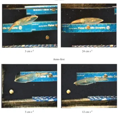
3 cm s-1 _{24 cm s}-1

3 cm s-1 12 cm s-1

Tail-first

Arms-first Fig. 2. Video frames of a 4.4 cm

dorsal mantle length Lolliguncula

brevis swimming tail-first at 3

mantle contraction and refilling (Fig. 3, Fig. 5B), whereas at higher speeds when fin activity was reduced, fin downstrokes frequently occurred during mantle contractions (Fig. 5A).

Although contraction rates during tail-first swimming did not increase significantly with speed for squid in the size classes 3.0–4.9 cm, 5.0–6.9 cm and 7.0–8.9 cm DML, mantle expansion did increase with speed (linear regressions, P<0.05; Fig. 6). However, no clear increase in mantle expansion with speed was detected for squid 1.0–2.9 cm in DML, the size class in which mantle contraction did increase with swimming speed. Mantle expansion of squid swimming in an arms-first orientation did not increase significantly with speed (Fig. 6). During tail-first swimming, vertical fin motion (the absolute vertical distance between maximum upstroke and maximum downstroke) decreased with increasing swimming velocity (linear regressions, P<0.05), but no detectable decrease in fin amplitude was found for arms-first swimming (Fig. 6).

The time required for mantle expansion during tail-first swimming was greater than that required to contract the mantle for squid in size classes 3.0–4.9 cm, 5.0–6.9 cm and 7.0–8.9 cm DML over the range of speeds considered (paired t-test, P<0.05) (Table 2). When data from all the size classes were pooled, this difference was highly significant (P=0.0002). When swimming in an arms-first orientation, only squid 3.0–4.9 cm in DML had greater mantle expansion than contraction times, but mantle expansion times were significantly greater than contraction times when data from all the size classes were pooled (P=0.0064) (Table 2). Mantle expansion time decreased with increased swimming speed only for squid 1.0–2.9 cm in DML while swimming tail-first (linear regression, P=0.0080; r2_=0.857) (Table 2). Mantle contraction time decreased with increasing swimming speed for squid 1.0–2.9 cm and 3.0–4.9 cm in DML while swimming tail-first (linear regression, P=0.0034, r2_{=0.907 for 1.0–2.9 cm DML;} P=0.0391; r2_{=0.535 for 3.0–4.9 cm DML) (Table 2).}

No significant differences between upward and downward fin stroke times were detected, and there was no increase or decrease in upward or downward fin stroke time with increasing speed for squid swimming in either tail-first or arms-first orientations (Table 2). Furthermore, no consistent increase or decrease in trailing edge fin speed with increasing swimming speed was detected when size classes were examined separately; however, when the size classes were pooled, a linear

increase in fin speed with increasing swimming velocity was detected for squid swimming tail-first (P=0.0151; r2_=0.461) (Table 2). Mean trailing edge fin speeds ranged from 4.2 to 12.3 cm s−1_{. At swimming speeds below 9 cm s}−1_{, trailing edge fin} speeds generally exceeded swimming speeds, and the trailing edge fin wave resembled a sideways ‘S’. At speeds of 9–12 cm s−1_{or above, trailing edge fin speeds were generally} less than swimming speed, and the trailing fin wave more closely resembled an inverted ‘V’, with the distal portion of the wave at an obtuse angle relative to the oncoming water flow. 5 10 15 20 25 30 Angle (de grees)

0 0.5 1 1.5 2

Arms Mantle -1 -0.5 0 0.5 1 V er tic al fi n m o tio n

0 0.5 1 1.5 2

1.5 1.55 1.6 1.65 Ma n tle d ia m et er ( cm )

0 0.5 1 1.5 2

-3 -2 -1 0 1 2 3 V el oci ty rel at iv e to free -s tre am f lo w ( cm s -1)

0 0.5 1 1.5 2

-30 -20 -10 0 10 20 30 40 A cc eler at io n ( cm s -2)

0 0.5 1 1.5 2

Time (s)

Fig. 3. Arm and mantle angles of attack, vertical fin motion (relative to the point where the fin connects to the mantle), mantle diameter, changes in linear velocity (relative to free-stream flow) and acceleration for a 4.4 cm dorsal mantle length (DML)

3665

Swimming mec

hanics and behaviour of

Lolliguncula bre

vis

Table 2. Summary of results of paired t-tests and linear regressions performed on kinematic data collected from Lolliguncula brevis swimming in tail-first and arms-first orientations over a range of speeds

Regression

Regression Regression of mean maximum Regression of

Paired of mantle of upward Regression positive (+) and mean maximum

comparison of Paired comparison expansion and and downward of trailing negative (−) speed acceleration (+) mantle expansion of upward and contraction times fin stroke times edge fin speed deviations (cm s−1_{) and deceleration (−)}

Size class and contraction downward fin (s) on swimming (s) on swimming (s) on swimming on swimming on swimming

(cm DML) Orientation times (s) stroke times (s) speed (cm s−1_{) speed (cm s}−1_{) speed (cm s}−1_{) speed (cm s}−1_{) speed (cm s}−1₎

1.0–2.9 T P=0.2856 P=0.0694 E: P=0.0080*; U: P=0.6667 P=0.3111 +: P=0.0824 +: P<0.0001*

r2_{=0.857; m=}−_{0.006 D: P=0.4065} −_{: P=0.0133* r}2_{=0.985; m=3.285}

C: P=0.0034* r2_{=0.818; m=−0.148 −: P=0.0003*}

r2_{=0.907; m=}−_{0.004 r}2_{=0.974; m=}−_4.446

1.0–2.9 A NA NA NA NA NA NA NA

3.0–4.9 T P=0.0095*; E >C P=0.4274 E: P=0.2783 U: P=0.2339 P=0.2833 +: P=0.0087* +: P=0.0008*

C: P=0.0391*; D: P=0.6143 r2_{=0.709; m=0.168 r}2_{=0.868; m=3.223}

r2_{=0.535; m=}−_0.0004 −_{: P=0.0088*} −_{: P=0.7374}

r2_{=0.708; m=−0.165}

3.0–4.9 A P=0.0463*; E>C P=0.3910 E: P=0.8236 U: P=0.8790 P=0.1048 +: P=0.3808 +: P=0.3660

C: P=0.7418 D: P=0.9418 −: P=0.9200 −: P=0.5479

5.0–6.9 T P=0.0245*; E>C P=0.3280 E: P=0.1126 U: P=0.4556 P=0.3155 +: P=0.0311* +: P<0.0007*

C: P=0.3157 D: P=0.2134 r2_{=0.612; m=0.193 r}2_{=0.824; m=2.834}

−: P=0.0439* −: P=0.0397*

r2_{=0.563; m=−0.152 r}2_{=0.555; m=−2.111}

5.0–6.9 A P=0.0663 P=0.3325 E: P=0.8863 U: P=0.4568 P=0.6143 +: P=0.5447 +: P=0.2894

C: P=0.7324 D: P=0.1838 −: P=0.1156 −: P=0.2252

7.0–8.9 T P=0.0119*; E>C P=0.3933 E: P=0.3362 U: P=0.7115 P=0.1554 +: P=0.2391 +: P=0.0293*

C: P=0.4155 D: P=0.7594 −: P=0.0897 r2_{=0.575; m=0.745}

−: P=0.9235

7.0–8.9 A P=0.0814 P=0.2038 E: P=0.1888 U: P=0.2116 P=0.7694 +: P=0.1097 +: P=0.7270

C: P=0.3437 D: P=0.2557 −: P=0.0659 −: P=0.4159

Pooled T P=0.0002*; E>C P=0.8596 E: P=0.8580 U: P=0.3347 P=0.0151; +: P=0.0004* +: P<0.0001*

C: P=0.4726 D: P=0.8263 r2_{=0.461; m=0.461 r}2_{=0.823; m=0.0183 r}2_{=0.904; m=3.297}

−: P=0.0039* −: P=0.0005*

r2_{=0.675; m=}−_{0.145 r}2_{=0.785; m=}−_2.586

Pooled A P=0.0064*; E>C P=0.3517 E: P=0.9473 U: P=0.8240 P=0.3601 +: P=0.6989 +: P=0.1449

C: P=0.8285 D: P=0.1931 −: P=0.0869 −: P=0.0975

The four size classes considered are as follows: 1.0–2.9 cm DML, 3.0–4.9 cm DML, 5.0–6.9 cm DML and 7.0–8.9 cm DML.

No statistical analyses were performed on squid in the smallest size class swimming in an arms-first orientation because of limited data. Asterisks denote significance at P<0.05.

When tail-first swimming data from the four size classes were pooled, mean maximum positive and negative (converted to absolute values) deviation in velocity and acceleration were found to increase with swimming speed (P<0.0039; r2_{>0.675) (Table 2).} Although linear relationships were not always detected when tail-first velocity and acceleration deviations were regressed against swimming speed and examined separately by size class, P-values of less than 0.10 were frequently observed (Table 2). No linear relationships between mean maximum velocity deviation and speed and mean maximum acceleration deviation and speed were detected for squid swimming in the arms-first orientation (P>0.05).

Flow visualization

On the basis of velocity measurements of particles expelled by squid during swimming, all three propulsion efficiencies were lowest at 3 cm s−1 _{and highest at 9 cm s}−1_{, and} arms-first propulsive efficiencies were generally higher than tail-first efficiencies (Table 3). Rocket motor propulsive efficiencies were consistently higher than Froude propulsion efficiencies and, on average, whole-cycle efficiencies were lower than both Froude and rocket motor propulsion efficiencies.

When dye or milk was injected into the mantle of squid (mean DML 4.2 cm), the squid appeared agitated and frequently jetted abruptly and erratically across the aquarium or into the aquarium walls. During these episodes, the jet wake was

generally very turbulent, and no vortex ring formation was observed. However, on several occasions, the squid swam across the aquarium (often beginning from rest), achieving a speed of 8.6±2.5 cm s−1_{, and several vortex rings formed} in the jet wake. The mean ring radius was 4.8±1.2 cm and the mean jet core radius was 2.6±0.8 cm (means ± S.D., N=2).

Obvious flow separation and the subsequent migration of flow along the body in a retrograde flow direction was observed when the mantle and arms of models were both positioned at more than 30 ° relative to flow, irrespective of whether the models were positioned tail- or arms-first. Separation was also observed when the leading body section,

i.e. the mantle when in the tail-first swimming mode or the arms when in the arms-first swimming mode, was at 0 ° and the trailing body section was positioned at more than 30 °. However, when the leading body section was at 10–20 °, separation did not occur until the trailing section was at 40 ° or more. During tail-first swimming, no squid positioned its mantle at a higher angle of attack than its arms, but during arms-first swimming, angles of attack of the arms were occasionally observed to be higher than those of the mantle. In flow visualization experiments using models oriented arms-first, separation occurred whenever the arms were at angles of attack 10–15 ° greater than that of the mantle.

0 1 2 3 4 5

0 5 10 15 20 25

0 1 2 3 4 5

0 5 10 15 20 25 0

1 2 3 4 5

0 5 10 15 20 25

0 1 2 3 4 5

0 5 10 15 20 25

Mantle contraction frequenc

y (s

-1)

F

in-b

eat frequenc

y (s

-1)

1.0–2.9 cm DML: y = 0.11x + 2.03, r2 = 0.98, P = 0.0002

Swimming speed (cm s-1₎

3.0–4.9 cm DML: y = −0.20x + 3.62, r2 _{= 0.86, P = 0.006} 5.0–6.9 cm DML: y = −0.17x + 2.96, r2 = 0.83, P = 0.007 7.0–8.9 cm DML: y = −0.11x + 2.94, r2 _{= 0.88, P = 0.0006}

1.0–2.9 cm DML 3.0–4.9 cm DML 5.0–6.9 cm DML 7.0–8.9 cm DML Tail-first Arms-first

Tail-first Arms-first

3667

Swimming mechanics and behaviour of Lolliguncula brevis

Force measurements

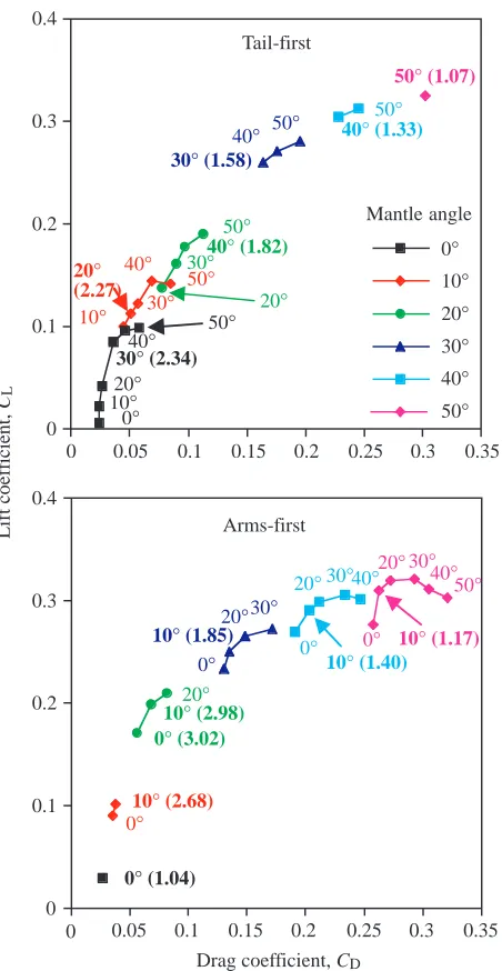
Polar diagrams of drag and lift coefficients calculated from squid models with extended fins positioned in both tail-first and arms-first orientations in a water tunnel are depicted in Fig. 7. The symbols displayed on the figure represent the various mantle angles of attack, while the degree designations in colour on the figures represent arm angles of attack. (Only mantle/arm

angle combinations observed in video footage of swimming squid were included in the figures.) For the mantle/arm angle combinations considered, the highest lift-to-drag ratios for tail-first swimming were detected at mantle/arm angle combinations of 0 °/30 ° (2.34) and 10 °/20 ° (2.27) (Fig. 7). The highest lift-to-drag ratios for arms-first swimming were detected at mantle/arm angles of 20 °/0 ° (3.02) and 20 °/10 ° 2.35

2.4 2.45 2.5 2.55 2.6

Mantle diameter (cm) 0 0.25 0.5 0.75 1 1.25 1.5 1.75 2

0 0.1 0.2 0.3 0.4 0.5 0.6

Fu

nnel diameter (cm)

0 0.25 0.5 0.75 1 1.25 1.5 1.75 2

-2 -1 0 1 2

V

ertical

fin m

o

ti

o

n (cm)

0 0.25 0.5 0.75 1 1.25 1.5 1.75 2

Time (s)

2.45 2.5 2.55 2.6 2.65 2.7

Mantle diameter (cm) 0 0.25 0.5 0.75 1 1.25 1.5 1.75 2

0 0.1 0.2 0.3 0.4

Fu

nnel diameter (cm)

0 0.25 0.5 0.75 1 1.25 1.5 1.75 2

-1.5 -1 -0.5 0 0.5 1 1.5

V

ertical

fin m

o

ti

o

n (cm)

0 0.25 0.5 0.75 1 1.25 1.5 1.75 2

Time (s)

A

B

Fig. 5. Mantle diameter, funnel diameter and vertical fin motion (relative to the point where the fin connects to the mantle) of a

Lolliguncula brevis (7.3 cm in dorsal

Table 3. Froude propulsion, rocket motor propulsion and whole-cycle propulsion efficiencies for Lolliguncula brevis swimming in both tail-first and arms-first orientations

Swimming speed Froude propulsion efficiency (%) Rocket propulsion efficiency (%) Whole-cycle propulsion efficiency (%)

(cm s−1_{) T A T A T A}

3 28.3 57.9 32.1 69.9 29.0 44.6

6 42.4 64.0 50.1 77.1 39.5 44.6

9 57.5 74.3 69.4 87.8 44.4 43.0

12 53.8 69.9 64.8 83.0 43.9 44.0

15 48.4 57.9 42.3

18 46.0 54.9 41.3

21 40.3 47.5 38.3

24 43.8 51.9 40.2

27 45.1 52.9 41.0

A, arms-first; T, tail-first.

Since the majority of squid did not swim at speeds above 12 cm s−1 _{in the arms-first mode, arms-first efficiencies were only calculated for}

speeds of 3–12 cm s−1_.

0 1 2 3

0 5 10 15 20 25 0 0.05 0.1 0.15 0.2 0.25 0.3

0 5 10 15 20 25

0 1 2 3

0 5 10 15 20 25 0.05

0.1 0.15 0.2 0.25 0.3

0 5 10 15 20 25

Mantle e

xpansion (cm)

Tail-first Arms-first

Tail-first _Arms-first

A

b

sol

u

te

v

er

tical

fin motion (cm)

Swimming speed (cm s-1) 3.0–4.9 cm DML: y = 0.002x + 0.10, r2 = 0.97, P < 0.0001 5.0–6.9 cm DML: y = 0.003x + 0.14, r2 _{= 0.97, P < 0.0001} 7.0–8.9 cm DML: y = 0.004x + 0.17, r2 _{= 0.92, P = 0.0002}

1.0−2.9 cm DML: y = −0.055x + 0.79, r2 = 0.67, P = 0.043 3.0−4.9 cm DML: y = −0.095x + 1.78, r2 = 0.79, P = 0.018 5.0−6.9 cm DML: y = −0.096x + 2.19, r2 _{= 0.75, P = 0.026} 7.0−8.9 cm DML: y = −0.13x + 3.43, r2 _{= 0.88, P = 0.0005}

1.0–2.9 cm DML 3.0–4.9 cm DML 5.0–6.9 cm DML 7.0–8.9 cm DML Fig. 6. Mantle expansion and vertical

fin motion (absolute vertical distance between maximum upstroke and downstroke) plotted over a range of swimming speeds for Lolliguncula

brevis swimming in both tail-first and

arms-first orientations. Data from four size classes are depicted: 1.0–2.9 cm, 3.0–4.9 cm, 5.0–6.9 cm and 7.0–8.9 cm dorsal mantle length (DML). When significant linear relationships were detected, regression lines were plotted, and regression equations, r2_{values and}

P values were included underneath

3669

Swimming mechanics and behaviour of Lolliguncula brevis

(2.98). On the basis of video footage of tail-first swimming, mean mantle/arm angle combinations over all size classes for low (3 cm s−1_{), intermediate (12 cm s}−1_{) and high (21 cm s}−1₎ speeds were 20.9 °/33.4 °, 10.1 °/17.8 ° and 8.7 °/10.7 °, respectively. Lift-to-drag ratios were therefore 1.78 for low speeds, 2.27 for intermediate speeds and 2.26 for high speeds. On the basis of video footage of arms-first swimming, mean mantle/arm angle combinations for low (3 cm s−1₎ and intermediate (12 cm s−1_{) speeds were 24.2 °/18.8 ° and}

8.8 °/6.3 °, respectively (squid did not swim arms-first at high speeds). Lift-to-drag ratios for low and intermediate speeds were 2.18 and 2.68, respectively. On the basis of force measurements collected from models with and without fins, the fins contributed 10–51 % of the total drag force and 0–65 % of the total lift force for mantle angles of attack between 0 and 40 ° during tail-first swimming and 15–61 % of the total drag force and 4–68 % of the total lift force for mantle angles of attack between 0 and 40 ° during arms-first swimming.

Added mass coefficients calculated from force measurements collected from squid models are plotted in Fig. 8. Added mass coefficients increased exponentially as the angle of attack of the mantle and arms increased, irrespective of whether the models were positioned in the tail-first or arms-first orientation.

Hydrodynamics

Resistive and propulsive forces acting on three squid (1.8 cm, 4.4 cm and 7.6 cm in DML) swimming tail-first and arms-first over a range of speeds are displayed in Table 4. For all three squid, buoyant weight was greater than lift and vertical jet thrust for swimming velocities at and below 12–15 cm s−1 (see negative values in vertical force balance column of Table 4 and balance of forces in Fig. 9). Fin thrust was not calculated directly, but the force imbalance between buoyant weight, lift and vertical jet thrust may serve as a good approximation of vertical fin thrust, especially since there was little net change in altitude from the beginning to the end of the video sequences (vertical change <0.9 cm; Table 4). On the basis of the vertical force imbalance, the potential contribution of the fins to upward-directed forces was substantial at low speeds (3–6 cm s−1_{), ranging from 28.4 to 78.6 % when models} with fins were considered in force balance equations and from 42.9 to 83.8 % when models without fins were considered. The contribution of the fins to upward-directed forces decreased with increasing speed. Fin activity ceased at 12, 15 and 18 cm s−1_{for 1.8, 4.4 and 7.6 cm DML squid, respectively, and} fin use predictions were in reasonable agreement with these speeds. For example, only 4.1 % of the upward-directed force by the 1.8 cm DML squid was unaccounted for and assumed to be generated by the fins at 12 cm s−1_{, when no fin activity was} employed.

The acceleration reaction was clearly the dominant instantaneous horizontal force (Fig. 9, Fig. 10). Although the mean acceleration reaction over a video sequence was low relative to the range of instantaneous acceleration reaction values within a series of jet cycles, mean values were nonetheless high and variable relative to the other forces (Table 4). The high variability is attributed to its sensitivity to velocity changes. Since the acceleration reaction should theoretically balance out over several jet cycles (Daniel, 1983), the horizontal force balance was calculated assuming that the mean acceleration reaction was zero for the video sequence. (If actual acceleration reaction forces were included in force balance equations, they would dominate the force balance and obscure fin thrust calculations.) On the basis of the horizontal force 0

0.1 0.2 0.3 0.4

0 0.05 0.1 0.15 0.2 0.25 0.3 0.35

0 0.1 0.2 0.3 0.4

0 0.05 0.1 0.15 0.2 0.25 0.3 0.35 Tail-first

Arms-first

L

ift

coe

ffi

ci

en

t,

CL

Drag coefficient, CD 0°

10° 20° 3040° (2.34)°

50° 10°

20° (2.27)

30° 40°

50° 20° 30°40° (1.82)

50°

30° (1.58)

40° 50° 40° (1.33)

50° 50° (1.07)

0° (1.04) 0°

10° (2.68) 0° (3.02)

1020°° (2.98)

0° 10° (1.85)

20°30°

0°

10° (1.40) 20°30°40°

0° 10° (1.17)

20°30° 40°

50° 0° 10° 20° 30° 40° 50° Mantle angle

balance equation, the fins appeared to contribute significantly to horizontal thrust, especially at low speeds (3–6 cm s−1_{) when the potential} contribution of the fins to horizontal thrust ranged from 32.0 to 55.1 % (Table 4). As was the case for vertical fin thrust predictions, horizontal fin thrust predictions based on force balance equations were in reasonable agreement with kinematic observations; predicted horizontal fin thrust was less than 5 % of the overall horizontal thrust when the fins were inactive (Table 4). A significant proportion of the drag in the horizontal direction was a product of positioning the mantle and arms at angles of attack greater than 0 °, especially at low speeds (3–6 cm s−1_{) when as much as 91.3 % of} the drag was associated with the angle of attack (Table 4).

Discussion

Lolliguncula brevis

The data from this study indicate that Lolliguncula brevis is a slow-swimming squid that relies heavily on its fins for locomotion, is capable of swimming in two different orientations and uses various swimming strategies depending on size. Unlike other squid, such as Loligo opalescens and Illex illecebrosus, which swim for sustained periods at speeds as high as 50 and 100 cm s−1_{, respectively} (Webber and O’Dor, 1986; O’Dor, 1988; O’Dor and Webber, 1991), L. brevis generally swims at speeds below 22 cm s−1 and swims either tail-first or arms-first at speeds below 9–15 cm s−1_{. Because of its} relatively low speed range, L. brevis may use its fins, muscular hydrostats that presumably operate effectively only at

low/moderate speeds because of muscle and support structure constraints (Kier, 1988; Kier, 1989; O’Dor and Webber, 1991), over a larger proportion of its speed range (0–18 cm s−1_{) than} Loligo opalescens or Illex illecebrosus. Consequently, the fins play a more integral role in locomotion. Moreover, not all size classes of squid appear to use the same swimming approaches, with smaller squid increasing contraction rates but keeping expelled water volume fairly constant with increasing speed, while larger squid do the opposite.

Lift and stability requirements at low speeds

As is the case with many squid species, L. brevis is negatively buoyant and consequently must generate lift to

maintain position in the water column, an energetic expense that is not trivial at low speeds [see Bartol et al. (Bartol et al., 2001b)]. An important mechanism used by brief squid for lift generation at low speeds is the elevation of mantle and arm angles of attack, which induce downward flow, enhance the pressure differential above and below the body and increase lift (Vogel, 1994; Dickinson, 1996). Although the mantle and arms of squid do not resemble traditional human-made airfoils, lift may be generated when the mantle (with attached fins) and arms are positioned at high attack angles (see polar diagrams). Lift enhancement by increasing body angles of attack has also been observed in negatively buoyant fish (He and Wardle, 1986; Webb, 1993), ski jumpers (Ward-Smith and Clements, 0

1 2 3 4 5 6 7 8 9 10 11 12 13 14 15 16

0 10 20 30 40 50 60

0 1 2 3 4 5 6 7 8 9 10 11 12 13 14 15 16

Tail-first

Added m

as

coe

ff

ic

ien

t,

CA

Arms-first

Mantle angle (degrees)

40°: y = 0.006x2− 0.037x + 1.00 0°

10° 20° 30° 40° 50° Arm angle

0° 10° 20° 30° 40° 50° Arm angle

r2 _{= 0.98, P = 0.006} 50°: y = 0.005x2_{− 0.047x + 1.03}

r2 = 0.97, P = 0.018

0°: y = 0.003x2_{− 0.047x − 0.029}

r2 = 0.95, P = 0.010 10°: y = 0.004x2− 0.001x + 1.08

r2 _{= 0.98, P = 0.018}

0 10 20 30 40 50 60

Fig. 8. Added mass coefficients (CA) for Lolliguncula brevis swimming in tail-first and arms-first orientations at various angles of attack. Mantle angles (degrees) are plotted on the

x-axes and arm angles are denoted using symbols. Only mantle/arm angle combinations

3671

Swimming mechanics and behaviour of Lolliguncula brevis

1982), honeybees (Nachtigall and Hanauer-Thieser, 1992), birds (Tobalske and Dial, 1996) and rays (Heine, 1992).

The trailing body section (i.e. the arms or mantle depending on swimming orientation) was frequently positioned at higher angles of attack than the leading body section. Flow visualization and lift measurement studies using squid models indicate that positioning the trailing body section at higher angles of attack than the leading body section delays flow separation (when coupled with appropriate leading body section angles) and elevates lift production during both tail-first and arms-tail-first swimming. This is analogous to control

surfaces on aircraft wings, such as ailerons or Fowler flaps, which are located on the trailing edge of the wing and positioned at higher angles of attack than the main wing (and often extended) to increase lift (Bertin and Smith, 1989; Kundu, 1990; Munson and Cronin, 1998). Just as pilots make fine lift adjustments with ailerons, squid in the tail-first swimming mode frequently adjusted the angles of attack of their arms (trailing body section) throughout the jet cycle and extended their arms to increase surface area, especially during refilling to generate extra lift when the jet was no longer producing any downward-directed thrust. At low speeds, the -0.003

-0.002 -0.001 0 0.001 0.002

0 0.25 0.5 0.75 1 1.25 1.5 1.75 2 5.2 5.4 5.6 5.8 6

0 0.5 1 1.5 2

-0.007 -0.005 -0.003 -0.001 0.001 0.003 0.005

0 0.25 0.5 0.75 1 1.25 1.5 1.75 2

F

orce (N)

Time (s) Vertical forces

Horizontal forces

H

ei

gh

t (c

m

)

Time (s)

Buoyant weight Lift

Vertical jet thrust Balance of forces

Drag

Acceleration reaction Horizontal jet thrust Refilling force Balance of forces