An Improvement on Data Driven Pole Placement for State Feedback Control and Model Identification

http://www.scirp.org/journal/ica ISSN Online: 2153-0661

ISSN Print: 2153-0653

An Improvement on Data-Driven Pole

Placement for State Feedback Control and

Model Identification

Pyone Ei Ei Shwe

1

, Shigeru Yamamoto

2

1_{Division of Electrical Engineering and Computer Science, Graduate School of Natural Science and Technology, Kanazawa University,} Kanazawa, Japan

2_{Faculty of Electrical and Computer Engineering, Institute of Science and Engineering, Kanazawa University, Kanazawa, Japan} Email: pyone@moccos.ec.t.kanazawa-u.ac.jp, shigeru@se.kanazawa-u.ac.jp

Abstract

The recently proposed data-driven pole placement method is able to make use of measurement data to simultaneously identify a state space model and de-rive pole placement state feedback gain. It can achieve this precisely for sys-tems that are linear time-invariant and for which noiseless measurement da-tasets are available. However, for nonlinear systems, and/or when the only noisy measurement datasets available contain noise, this approach is unable to yield satisfactory results. In this study, we investigated the effect on data-dri- ven pole placement performance of introducing a prefilter to reduce the noise present in datasets. Using numerical simulations of a self-balancing robot, we demonstrated the important role that prefiltering can play in reducing the in-terference caused by noise.

Keywords

Data-Driven Control, State Feedback, Pole Placement, Nonlinear Systems

1. Introduction

In state feedback pole placement, the state feedback gain must be determined for a given system such that the closed-loop poles coincide with the desired loca-tions. This is a well-known problem, and the pole placement methods have been extensively discussed in the literature [1][2][3][4]. In standard pole placement methods, a state space model is assumed to be given by a system identification technique using data from past experiments. Whereas the traditional approach combines the identification of the state space model with the standard pole placement method; an alternative approach called “data-driven pole placement”

How to cite this paper: Shwe, P.E.E. and Yamamoto, S. (2017) An Improvement on Data-Driven Pole Placement for State Feed-back Control and Model Identification. Intelligent Control and Automation, 8, 139-153.

http://dx.doi.org/10.4236/ica.2017.83011

Received: May 25, 2017 Accepted: July 15, 2017 Published: July 18, 2017

Copyright © 2017 by authors and Scientific Research Publishing Inc. This work is licensed under the Creative Commons Attribution International License (CC BY 4.0).

http://creativecommons.org/licenses/by/4.0/

has recently been proposed [5]. In this approach, the state space model and pole placement feedback gain are identified simultaneously from the set of state measurements and control input sequences. The method proposed in [5] is based on the data-driven control framework ([6] and references therein) such as unfalsified control [7], virtual reference feedback tuning (VRFT) [8][9], or ficti-tious reference iterative tuning (FRIT) [10] [11] [12] [13]. In the data-driven control framework, where no explicit mathematical plant model is used, a feed-back controller must be derived that satisfies the prescribed closed-loop perfor-mance and fits to known experimental data. In contrast with traditional mod-el-based controller designs, techniques such as controller identification [14] or a combination of plant model and controller identification must be applied [15] [16].

Many studies of data-driven control have focused on output feedback control and data-driven state feedback control [11] [12] [13], in which the prescribed closed-loop performance is achieved by applying a closed-loop reference transfer function. Such methods can be applied to the data-driven pole placement prob-lem by choosing a reference transfer function with the desired poles. However, the zeros of the reference transfer function cannot normally be specified, because the zeros of the plant are unknown. In contrast, the data-driven pole placement method presented in [5] requires only a state space representation of the closed- loop system to specify the prescribed closed-loop performance, as shown in Sec-tion 2. This avoids the zero assignment issue that arises in the transfer funcSec-tion approach used in [5].

This data-driven pole placement method can, therefore, be applied to linear and time-invariant systems with measurable states. The method is briefly re-viewed in Section 2. However, the capacity of the data-driven pole placement method to handle noise remains an open issue, though in [5], the total least square (TLS) method [17] was claimed to be effective. Measurement noise is one of the issues which may surely face in practical applications. Therefore, to re-solve this, we introduced a prefiltering technique that reduces the effect of mea-surement noise in Section 3. More specifically, a finite impulse response (FIR) filter is used to prefilter the data, as this makes them easier to manipulate. In Section 4, by using the numerical example of a self-balancing robot, we discuss the effect of applying this prefiltering technique, together with the least square (LS) and TLS methods, to a self-balancing robot model. We investigate the abili-ty of the data-driven pole placement method to produce a linearized model us-ing numerical simulations as in [18]. A nonlinear differential equation was used to represent the dynamics of a self-balancing robot there. Moreover, we evaluate the effects by two different exciting signals, the random and the chirp exciting signal, along with TLS and prefiltering. Finally, we compare all the results for the pole placement error and identification error when two exciting signals are ap-plied.

Notation: Let A and B be m n× and p q× matrices, respectively. Then,

11 1

1

,

n

m mn

a B a B

A B

a B a B

 

 

⊗ =  

 

 



 



(1)

where a i_ij( =1,, , 1,m j= , )n is the _ijth element of _A. The vectorization of then stacks the columns into a vector:

( )

1

vec ,

n a

A

a

    =      



(2)

in which aj is the th

j column of A . The Frobenius norm of matrix m n

A∈R × is defined as

2 1 1

.

m n ij F

i j

A a

= =

=

∑∑

(3)

2. Data-Driven Pole Placement

In this section, we briefly review the data-driven pole placement method formu-lated in [5].

Consider a discrete-time linear time-invariant system and static state feedback

(

1

)

( )

( )

x k+ =Ax k +Bu k (4)

( )

( ) ( )

u k =Fx k +v k (5)

where _A∈n n× ,_B∈n m× ,_x∈n _{is the state vector,} m

u∈ is the input vector,

m n

F∈ × is the feedback gain, and v∈m is the external input to the closed

loop system.

The data-driven pole placement problem was formulated in [5] as follows: Problem 1. We assume that the order of the plant n is known, state n is mea-surable, pair

(

A B,

)

is controllable but the exact value is unknown and B is

of full rank. Let Λ=

{

p1,,pn

}

be a self-conjugate set of n complex numbers

in the unit circle. Given the input and output measurement data sequence

( ) ( )

(

x k u k0 , 0

)

of (4), find a state feedback gain F from the observed data

( ) ( )

(

x k u k0 , 0

)

such that

{

λ

i

(

A BF+

)

}

=Λ .

In a conventional approach, this problem is solved in two steps: A and B are identified from

(

x k u k0

( ) ( )

, 0

)

, then F is derived using the standard pole

placement algorithms. In contrast, the data-driven pole placement method solves the two steps simultaneously. To achieve this, the method uses the equivalency between the closed-loop system

(

1

) (

) ( )

( )

,

x k+ = A+BF x k +Bv k (6) with the desired pole placement gain F and

(

)

( )

( )

d 1 d d d ,

x k+ =A x k +B v k ₍₇₎

( )

( )

d ,

x k =Tx k (8)

from (7) by using (5), to obtain

(

)

( )

( )

( )

d 1 d d d d .

x k+ =A x k +B u k −B Fx k

₍₉₎

Then, using (8), we obtain

(

1

)

d

( )

d

( )

d

( )

.

Tx k+ =A Tx k +B u k −B Fx k ₍₁₀₎

If

(

x k u k0

( ) ( )

, 0

)

(

k=i,,i+N

)

satisfies (10),

0 1 d 0 2 d 0 d 0,

TX P=A TX P +B U −B FX (11)

where

( ) ( )

(

)

0 0 0 1 0 ,

X =_x i x i+ x i+N _

(12)

( ) ( )

(

)

0 0 0 1 0 1 ,

U =_u i u i+ u i+ −N _

(13)

1

1 2

1

0

, . 0

N N

N N

I

P P

I ×

×

   

=_{ } =_{ }

    (14)

In [5], Equation (11) is cast into

1 0 1 2 0 2 d 0,

T T

S X P S X P B U

F F

   

+ =

   

    (15)

[

]

[

]

1 n 0n m , ,2 d d

S = I × S = −A B ₍₁₆₎

and

1 1

, .

m n n n

m m

f t

F T

f t

× ×

   

   

=_{ }∈ =_{ }∈

   

   

    (17)

Remark 1. The system in (7) can be interpreted as a reference model within VRFT (e.g., [8][9]) and FRIT (e.g., [10][11][12][13]). The idea of eliminating v in (9) is also based on FRIT. In[10][11][12], a similar state feedback control problem has been discussed within the FRIT framework. To apply these FRIT techniques to the data-driven pole placement problem, the desired transfer func-tion must be specified from u to x, rather than x_d. When precise values for

(

A B,

)

are not available, it becomes impossible to specify the zeros of the

de-sired transfer function.

Remark 2. To obtain the datasets in (12) by applying state feedback in (5) to the system in (4), the initial feedback gain F should be based on

(

A B,

)

.

Hence, in Problem 1, the exact value of

(

A B,

)

is assumed to be unknown.

When applying the property of Kronecker product

(

)

(

)

vec MND = NT ⊗M vec D (see for example Th.2.13 in [19]) to the

trans-pose of (15) to solve (15) for F and T, a further linear equation is derived, as follows:

,

η

Χ =U ₍₁₈₎

where

[

]

( )

1 1 ,

n m n

n m

t t f f

η

_{=  } Τ_∈ +

(

)

(

)

( )

1 0 1 2 0 2 ,

nN n m n

S X P Τ S X P Τ × +

Χ = ⊗ + ⊗ ∈_

(20)

(

d 0

)

(

vec .

)

nN m

B UΤ I

= ⊗ ∈_

U (21)

If T is nonsingular, the model coefficients can be obtained

1 1 1

d d , d.

A=T−A T−T B F− B=T B− ₍₂₂₎

3. Prefiltering Noisy Measurement

When the measurement of x is contaminated by noise ε,

( )

( )

( )

0 .

x k =x k +ε k

₍₂₃₎

Then, (10) becomes

(

) (

)

(

)

( ) ( )

(

)

( )

(

( ) ( )

)

0

d 0 d 0 d 0

1 1

.

T x k k

A T x k k B u k B F x k k

ε

ε

ε

+ − +

= − + − − (24)

Hence, if

(

x0

( ) ( )

k u k, 0

)

(

k=i,,i+N

)

satisfies the above equation,

(

)

(

)

(

)

0 1

d 0 2 d 0 d 0 2,

T X E P

A T X E P B U B F X E P

−

= − + − − (25)

where

( ) ( )

1

(

)

.

E=_

ε

i

ε

i+ 

ε

i+N _

(26) Then, the resulting linear equation is given as

(

Χ + ∆Χ

)

η=U+ ∆U, ₍₂₇₎

where the effect of noise ∆Χ has the same structure as Χ in (20), then

( )

T

( )

T

1 1 2 2 ,

S EP S EP

∆Χ = − ⊗ − ⊗

(28) and ∆U is the equation error. Following [5], we can solve

η

∈R(n m n+ ) to

(27) as a TLS problem [17], by minimizing the Frobenius norm

[

∆Χ ∆U

]

_F. It is known that the TLS solution is given as

12 22

1

V V

η = −

(29) based on the singular value decomposition

[

] [

]

1 11 12 T

2 21 2

2 1

2

0

, 0

V V

V V

Σ

   

Χ _{   }

Σ

  

=



U U U

(30) where these matrices are partitioned into blocks corresponding to Χ and U.

Here, we assume that there exists M >0 such that

(

)

1

1

0

M

j

i j

M =ε

+ ≈

∑

(31) for all i. This means that when

N

>

M

,

1 0, 02

EPΦ ≈ EPΦ ≈ ₍₃₂₎

( 1)

1 0 0

1 0

1

,

0 1

0 0 1

N N M

M

× − +

 

 

 

 

Φ =  ∈

 

 

 

 

 

    

 

  

   



(33)

where each column has M elements of 1. Therefore,

0 1 d 0 2 d 0 d 0 2

TX P =A TX P +B U −B FX P ₍₃₄₎ where

0 0 , .0 0

X =X Φ U =U Φ ₍₃₅₎ This multiplication by Φ represents the prefiltering of signals via an

M

th

order FIR filter.

When the systems (4) and (7) are driven by the exciting signal, we have

(

X0−E P

)

1=A X

(

0−E P

)

2+BU0, (36)

(

)

0 0 2 ,

U =F X −E P +V

₍₃₇₎

(

)

d 0 2,

X =T X −E P (38)

d 1 d d 2 d ,

X P =A X P +B V (39)

where

( )

( )

(

)

d d d 1 d ,

X =_x i x i+  x i+N _ (40)

( ) ( )

1

(

1 .

)

V =_v i v i+  v i+ −N _ (41)

By applying Φ _{to these systems, we obtain}

0 1 0 2 0 ,

X PΦ =AX PΦ +BU Φ (42)

0 0 2 ,

U Φ =FX PΦ + ΦV (43)

d 2 0 2 ,

X PΦ =TX PΦ (44)

d 1 d d 2 d .

X PΦ =A X PΦ +B VΦ (45)

Here, if VΦ ≈0, (34) cannot be satisfied. Hence, for all i, VΦ ≠0, that is

(

)

1

1

0

M

j

v i j

M =

+ ≠

∑

(46)

must be satisfied.

4. Numerical Example: Self-Balancing Robot

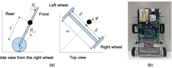
We next applied the data-driven pole placement method described above to the model of a self-balancing robot [21] [20] as shown in Figure 1. The robot is equipped with right and left wheels driven by direct current (DC) motors whose voltages vr and v1 can be controlled. Because the motion dynamics can be

decomposed by the input u, the control input to the robot was represented as

1 1

2 1

.

r

r

u v v

u

u v v

+

   

=_{  }= _

−

[image:7.595.211.541.68.199.2]

Figure 1. (a) Coordinates of the self-balancing robot; (b) photo.

We assume that the pitch angle θb and the pitch angular velocity θb of the body could be measured, as well as the angles θr and θ1 of the right and left

wheels, and their angular velocities θr and θ1, respectively. We define the mean values of the right and left wheel angles θr and θ1, and the yaw angle of

the body as follows:

(

)

w r 1

1

, 2

θ

=

θ θ

+ ₍₄₈₎

(

r 1

)

,

r w

φ

=

θ θ

− ₍₄₉₎

where r is the radius of the wheel and

w

=

2

d

is the distance between the two wheels.

4.1. Equation of Motion

The equation of motion for the self-balancing robot can be derived as

( )

(

)

_{( )}

( )

_{( )}

( )

( )

( )

_{( ) ( )}

( )

( )

(

)

( )

( )

(

( )

( )

)

( ) ( )

( )

2

w w b

1 b 1 b b 2 1

b b b

2

2 b 2 b b b b 2

sin

cos

2 sin cos ,

t t r t

J t D M l t H u t

t t g l t t

J t t D t M l t t t t H u t

θ

θ

θ

θ

θ

θ

θ

θ

φ

θ

φ

φ

θ

θ

θ

φ

       + − =         _{     + }         _{+ + =}            (50) where

( )

(

w r2 m

)

(

w b

)

2 r2 m b b

1 b 2 2 2

r m b b b r m b

2 2 2 cos

,

2 cos 2

J g J M M r g J M lr

J

g J M lr J g J M l

θ θ θ  + + + − +  =   − + + +    

( )

2

(

2

)

2 2 2

2 b 2 2 w r m 2 w b sin b,

d

J J J g J M d M l

r

φ

θ

= + + + +

θ

b w b

1

b w b

2 d d d ,

D

d d d

+ −

 

= _{− −} 

 

(

)

2

2 2 2 b w ,

d

D d d

r = + 1 v 1 0 , 1 0

H = b  _

−

  2 v

[

0 1 ,

]

d

H b

r

=

2 r t e

b r m

m

: g K K ,

d g d

R

= + r t

v m

: g K .

b R

=

[image:8.595.210.541.88.361.2]

Table 1. Parameters of the self-balancing robot [20][21].

9.81

g= acceleration due to gravity [m/s2]

b 0.5

M = mass of body [kg]

w 0.07

M = mass of wheel [kg]

0.025

r= radius of wheel [m]

5

w 8.75 10

J = × − moment of inertia of wheel [kg∙m2]

2 0.12

w= d= vehicle width [m]

0.1073

l= distance from wheel center to center of gravity of robot body [m]

3

b 6.7 10

J = × − moment of inertia of body (pitch) [kg∙m2]

4

6 10

Jφ −

= × moment of inertia of body (yaw) [kg∙m2_]

4

m 1.3 10

J = × − moment of inertia of DC motor [kg∙m2]

m 0.035

R = resistance of DC motor [Ω]

e 0.02

K = electromotive force constant of DC motor [V∙s/rad]

t e

K =K torque constant of DC motor [N∙m/A]

r 30

g = gear ratio

m 0.0022

d = coefficient of friction between wheel and DC motor

w 0

d = coefficient of friction between wheel and floor

4.2. Linear Model and Feedback Gain

We linearized the equations of motion (50) around equilibrium states θ =w 0,

b 0

θ = _,

φ

=0, θ =_w 0, θb =0, φ = 0, and u=0. Then, under the assump-tion thatsinθb

( )

t ≈θb

( )

t , cosθb

( )

t ≈1,

( )

2 b

sin

θ

t ≈0,

θ

b2

( )

t ≈0,

( )

2

0

t

φ

≈ , andsin

θ

b

( )

t cos

θ

b

( ) ( )

t

φ

 t ≈0, the linearized equations of motion can be

de-rived as

( )

( )

( )

( )

( )

( )

( )

1 1 1 1

2 2 2 ,

a a a

b b

J x t D x t K x t H u t

J x t D x t H u t

+ + =   + =   

  (51)

where

( )

w

_{( )}

( )

( )

( )

b b

: , : ,

a

t

x t x t t

t θ φ θ   =_{ } =

  (52)

( )

( )

1 1 2 2 1 b

0 0 0 , 0 , lg .

0 1

J =J J =J K =M _ _

−

  (53)

By defining the state vector

( )

( )

_{( )}

( )

( )

( )

( )

w b 1 w b , a a t

x t t

x t

x t t

t θ θ θ θ      _{  } =_{  }= _  _{  }       

( )

( )

_{( )}

( )

_{( )}

2 , b b

x t t

x t

x t t

φ

φ

   

=_{  }= _

    (54)

the linear state space model can be derived as

( )

( )

( )

( )

( )

( )

1 1 1 1 1

2 2 2 2 2

, ,

c c

c c

x t A x t B u t

x t A x t B u t

= +   = +  

where

2 2 2

1 1 1

1 1 0 , c I A

J K J D

× − −   = _{− −}    2 1 1 1 v 1 0 , 1 1 c B b J × −     =_  _    _{ }−    2 1 2 2 0 1 , 0 c A

J −D

 

=  ₋ 

  2 1

v 2 0 . c B _d b J r −     =_{ }    

Then, the feedback can be independently designed as

1 1 1 1, 2 2 2 2.

u =F x +v u =F x +v ₍₅₆₎

Note that this can be more succinctly represented as

( )

( )

( ) ( )

( ) ( )

1

( )

_{( )}

2

, , ,

c c

x t

x t A x t B u t u t Fx t x t

x t

 

= + = _{=  }

 

 (57)

1 4 2 1 4 1 1 1 2

2 4 2 2 1 2 1 4 2

0 0 0

, , .

0 0 0

c c

c c

c c

A B F

A B F

A B F

× × ×

× × ×

     

=_{ } =_{ } =_{ }

 

    (58)

When the parameters in Table 1 are used and the sampling period is

0.1 s

h= , the discrete-time model after discretizing (55) is

(

)

( )

( )

(

)

( )

( )

1 1 1 1 1

2 2 2 2 2

1 ,

1 ,

x k A x k B u k

x k A x k B u k

+ = +

 

+ = +



(59)

where

1 1

1 0.1719 0.0226 0.0830 0.0641 0 1.1722 0.0113 0.0944 0.0094

, ,

0 3.5363 0.1388 1.0332 0.7131 0 3.5299 0.1386 1.0336 0.1148

A B       ₋      = =       ₋      2 2

1 0.0113 0.0306

, .

0 0.0001 0.3450

A =_ _ B =_ _

    (60)

Here, we assume that the exact values of (60) are not available, but that un-certain values are available:

1 1

1 0.1897 0.0218 0.0844 0.0648 0 1.1900 0.0115 0.0947 0.0095

, ,

0 3.9115 0.1408 1.0489 0.7115 0 3.9151 0.1407 1.0492 0.1165

A B       ₋      = =       ₋      2 2

1 0.0103 0.0310

, .

0 0.0001 0.3450

A =_ _ B =_ _

    (61)

The coefficients can be derived from J J1, 2, with an assumed uncertainty of

10%. By applying linear quadratic optimal control theory to (61), the desired closed-loop pole locations can be chosen as

(

)

{

5

}

1 1 1 1 6.0355 10 , 0.5253, 0.5745, 0.7630

A B F

λ _{+ ∈ Λ = ×} − , (62)

(

)

{

5

}

2 2 2 2 6.0426 10 , 0.7835

A B F

and the initial feedback gains needed to obtain datasets for the data-driven pole placement as

[

]

[

]

1 1.5216 124.181 2.3915 18.3089 , 2 6.2764 0.0646 .

F = F = − − (64)

4.3. Comparison of Methods

Next, simulations were conducted and comparisons were made from the ob-tained results when using different methods and exciting signals.

Measurement noise was prepared with the Gaussian distribution _N

(

_0,σ2

)

,

where 2 3

1.0 10

σ _{= ×} − _, 4

1.0 10× − and 1.0 10× −4 in θw, θb, and

φ

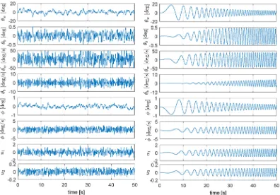
, respec-tively. This is shown in Figure 2(a). We used the random exciting signal v shown in Figure 3(a) and the linear chirp signal v k

( )

shown in Figure 3(b)

with the uniform distribution v k1

( )

U

(

−0.5, 0.5

)

and v2

( )

k U

(

−0.1, 0.1

)

. We set the order of the prefilter Φ (33) as M=6. After prefiltering, the

measurement noise in θw, θb, and

φ

was reduced, as shown in Figure 2(b). The prefiltered exciting signals were shown in Figure 3(b) and Figure 3(d). It can be seen that the exciting signals v were not eliminated by prefilter Φ, but that the high-frequency elements were reduced.

A closed-loop response in the presence of measurement noise by state feed-back (56), with initial gain (64), is shown in Figure 4. The response to the ran-dom exciting signal and the chirp exciting signal are shown in Figure 4(a) and Figure 4(b), respectively. Of particular note is that the responses of θb, θw, and θb in Figure 4(b) show the high-pass filter-like gain characteristics of the transfer function from v to x.

For comparison, the dataset for the data-driven pole placement was chosen as

( ) ( )

(

)

{

0 0

}

50, ,450

,

k

x k u k

=  where i=50 and N =400.

To evaluate the obtained pole placement gain F, we introduced an accuracy

measurement that takes the largest absolute difference in value between each ei-genvalue of Ai+B Fi i and the corresponding pj∈ Λi,

( )

Adi : max

{

j

(

Ai B Fi i

)

p pj j i

}

.

δλ

=

λ

+  − ∈ Λ

(65)

[image:11.595.175.540.68.280.2]

Figure 3. Exciting signal v (a) random, (b) chirp, (c) prefiltered random, (d) prefiltered chirp.

Figure 4. Closed-loop response by an initial state feedback via (a) random exciting signal v, (b) chirp

ex-citing signal v.

To evaluate the obtained model

(

A B ,

)

, the following identification errors

were used:

: , ,

i i i i i i

A A A B B B

∆ =  − ∆ =  −

(66)

( )

A_i : max

{

_j

( )

A_{i j}

( )

A_i

}

.

δλ = λ −λ  (67)

[image:11.595.143.539.309.585.2]

“sort”. This further sorts elements of equal magnitude by the phase angle on the interval

(

−π, π

]

. The impulse response

( )

(

)

1

G z = zI−A − B was used to eva-luate the model obtained, as follows:

( )

( )

10 2 , , 0 : , i i i i

i A B A B

k

G x k x k

=

∆ =

∑

  − (68)

where xA B _i, _i and xA Bi, i are the impulse responses of

( )

(

)

1

:

i i i

G z = zI−A − B and

( ) (

)

1

:

G z = zI−A − B, respectively.

From the perspective of system control, smaller is better, particularly in the case of δλ

( )

Adi , δλ

( )

Ai , and ∆Gi. The following key results were contras-tively found in Table 2:

1) The initial model and feedback gain were affected by uncertainty: The model errors and pole placement errors are shown in Table 2 (initial).

2) The results when using the LS method to solve linear Equation (27) for noiseless data are shown in Table 2(a). All errors were reasonably small, confirming that the data-driven method performs well when the measure-ment data

(

x k u k0

( ) ( )

, 0

)

are noiseless.

3) The results when using the LS method to solve linear Equation (27) for noisy data are shown in Table 2(b). All errors became larger when noise was added, suggesting that LS analysis is inadequate when the measurement data are contaminated by noise.

4) The results when using the TLS method to solve linear Equation (27) are shown in Table 2(c). The errors were significantly smaller than those re-ported in [5], using the LS method.

[image:12.595.206.540.469.732.2]

5) The results when applying prefiltering (PF) and using the TLS method to

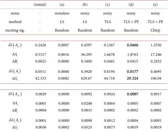
Table 2. Comparison of errors.

(initial) (a) (b) (c) (d) (e)

noise - noiseless noisy noisy noisy noisy

method - LS LS TLS TLS + PF TLS + PF

exciting sig. - Random Random Random Random Chirp

( )

Ad1

δλ _{0.2426 0.0007 0.4597 0.1367 0.0466 1.2530}

1 A ∆ 1 B ∆ 0.5317 0.0025 0.0016 0.0000 36.295 0.3400 1.6678 0.0481 1.8763 0.0415 17.246 0.2932

( )

A1

δλ 1 G ∆ 0.0511 42.333 0.0000 0.0082 0.3920 629.67 0.0194 44.718 0.0177 29.324 0.4695 106.04

( )

Ad2

δλ 0.0029 0.0000 0.0092 0.0024 0.0007 0.0017

2 A ∆ 2 B ∆ 0.0001 0.0004 0.0000 0.0000 0.0288 0.0031 0.0064 0.0002 0.0005 0.0002 0.0007 0.0002

( )

A2

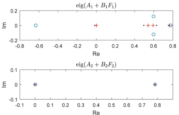
[image:13.595.233.525.67.255.2]

Figure 5. Comparison of pole locations (“+” indicates the desired poles, “.” those ob-tained by the random exciting signal and “o” those obob-tained by the chirp exciting signal.).

solve linear Equation (27) are shown in Table 2(d). The prefilter further re-duced the errors, in particular, the pole placement error δλ

( )

Ad1 and the impulse response error ∆G1.

6) The results when applying PF and using the TLS method to solve the li-near Equation (27), but with v as the chirp signal, are shown in Table 2(e). No significant improvement in error rates was found with respect to A2

when using the chirp exciting signal. However, the errors with respect to A1

became significantly worse than when a random exciting signal was used. This was assumed to be because A1 has an unstable eigenvalue of 1.7838. We

conclude that a random exciting signal is more appropriate than a chirp ex-citing signal when using data-driven methods.

Finally, we compare the pole locations obtained as shown in Figure 5. As can be seen, a better performance was achieved when using the random exciting signal.

5. Conclusion

In this study, we evaluated the different approaches reducing the effect of mea-surement noise in data-driven pole placement methods for deriving a state space model and pole placement state feedback. Using numerical simulations of a self-balancing robot, which is a nonlinear system, we demonstrated the important role that prefiltering can play in reducing the interference caused by noise. Again using numerical simulation, we compared the use of two exciting signals: a ran-dom signal and a chirp signal. The use of a ranran-dom exciting signal was found to be more effective with our proposed method. Further developments are needed in the methods used to cope with noise. A method such as that used in [9] may be appropriate for use in practical applications where noise is present, and adaptive control based on real-time updating [22] is a future promising approach.

Acknowledgements

References

[1] Wonham, W.M. (1967) On Pole Assignment in Multi-input Controllable Linear Systems. IEEE Transaction on Automatic Control, 12, 660-665.

https://doi.org/10.1109/TAC.1967.1098739

[2] Ackermann, J.E. (1977) On the Synthesis of Linear Control Systems with Specified Characteristics. Automatica, 13, 89-94.

[3] Kimura, H. (1975) Pole Assignment by Gain Output Feedback. IEEE Transaction Automatic Control, 20, 509-516. https://doi.org/10.1109/TAC.1975.1101028

[4] Hikita, H., Koyama, S. and Miura, R. (1975) The Redundancy of Feedback Gain Matrix and the Derivation of Low Feedback Gain Matrix in Pole Assignment. The Society of Instrument and Control Engineers, 11, 556-560. (In Japanese)

[5] Yamamoto, S., Okano, Y. and Kaneko, O. (2016) A Data-driven Pole Placement Method Simultaneously Identifying a State Space Model. Transaction of the Insti-tute of Systems, Control and Information Engineers, 29, 275-284. (In Japanese) [6] Hou, Z.S. and Wang, Z. (2013) From Model-Based Control to Data-Driven Control:

Survey. Classification and Perspective, Information Sciences, 235, 3-35.

[7] Safonov, M.G. and Tsao, T.C. (1997) The Unfalsified Control Concept and Learn-ing. IEEE Transactions on Automatic Control, 42, 843-847.

https://doi.org/10.1109/9.587340

[8] Campi, M.C., Lecchini, A. and Savaresi, S.M. (2002) Virtual Reference Feedback Tuning: A Direct Method for the Design of Feedback Controllers. Automatica, 38, 1337-1346.

[9] Sala, A. and Esparza, A. (2005) Extensions to “Virtual Reference Feedback Tuning: A Direct Method for the Design of Feedback Controllers”. Automatica, 41, 1473- 1476.

[10] Souma, S., Kaneko, O. and Fujii, T. (2004) A New Method of a Controller Parame-ter Tuning Based on Input-output Data-Fictitious Reference IParame-terative Tuning. Pro-ceedings of the 2nd IFAC Workshop on Adaptation and Learning in Control and Signal Processing, 37, 789-794.

[11] Matsui, Y., Akamatsu, S., Kimura, T., Nakano, K. and Sakurama, K. (2011) Ficti-tious Reference Iterative Tuning for State Feedback Control of Inverted Pendulum with Inertia Rotor. SICE Annual Conference, Tokyo, 13-18 September 2011, 1087- 1092.

[12] Matsui, Y., Akamatsu, S., Kimura, T., Nakano, K. and Sakurama, K. (2014) An Ap-plication of Fictitious Reference Iterative Tuning to State Feedback, Electronics and Communications in Japan, 97, 1-11. https://doi.org/10.1002/ecj.11506

[13] Kaneko, O. (2015) The Canonical Controller Approach to Data-Driven Update of State Feedback Gain. Proceedings of the 10th Asian Control Conference 2015 (ASCC 2015), Kota Kinabalu, 31 May-3 June 2015, 2980-2985.

https://doi.org/10.1109/ASCC.2015.7244744

[14] Van Heusden, K., Karimi, A. and Soderstrom, T. (2011) Extensions to “On Identi-fication Methods for Direct Data-Driven Controller Tuning”. International Journal of Adaptive Control and Signal Processing, 25, 448-465.

https://doi.org/10.1002/acs.1213

[15] Kaneko, O., Miyachi, M. and Fujii, T. (2008) Simultaneous Updating of a Model and a Controller Based on the Data-Driven Fictitious Controller. 47th IEEE Confe-rence on Decision and Control,Cancun, 9-11 December 2008, 1358-1363.

Controller Based on Fictitious Reference Iterative Tuning. SICE Journal of Control, Measurement, and System Integration, 4, 63-70. https://doi.org/10.9746/jcmsi.4.63 [17] Markovsky, I. and Huffel, S.V. (2007) Overview of Total Least-Squares Methods.

Signal Processing, 87, 2283-2302.

[18] Shwe, P.E.E. and Yamamoto, S. (2016) Data-Driven Method to Simultaneously Ob-tain a Linearized State Space Model and Pole Placement Gain. Proceedings of the 3rd Multi Symposium on Control Systems, Nagoya, 7-10 March 2016, 3B3-2. [19] Brewer, J. (1978) Kronecker Products and Matrix Calculus in System Theory. IEEE

Transactions on Circuits and Systems, 25, 772-781.

https://doi.org/10.1109/TCS.1978.1084534

[20] ZMP Inc. Stabilization and Control of Stable Running of the Wheeled Inverted Pendulum, Development of Educational Wheeled Inverted Robot e-nuvo WHEEL ver.1.0. http://www.zmp.co.jp/e-nuvo/

[21] Nomura, T., Kitsuka, Y., Suemitsu, H. and Matsuo, T. (2009) Adaptive Back Step-ping Control for a Two-Wheeled Autonomous Robot. Proceedings of ICCAS-SICE, Fukuoka, 18-21 August 2009, 4687-4692.

[22] Shwe, P.E.E. and Yamamoto, S. (2016) Real-Time Simultaneously Updating a Li-nearized State-Space Model and Pole Placement Gain. Proceedings of SICE Annual Conference, Tsukuba, 20-23 September 2016, 196-201.

Submit or recommend next manuscript to SCIRP and we will provide best service for you:

Accepting pre-submission inquiries through Email, Facebook, LinkedIn, Twitter, etc. A wide selection of journals (inclusive of 9 subjects, more than 200 journals)

Providing 24-hour high-quality service User-friendly online submission system Fair and swift peer-review system

Efficient typesetting and proofreading procedure

Display of the result of downloads and visits, as well as the number of cited articles Maximum dissemination of your research work