Electronic Band Structure of Graphene Based on the Rectangular 4 Atom Unit Cell

ISSN Online: 2153-120X ISSN Print: 2153-1196

Electronic Band Structure of Graphene

Based on the Rectangular 4-Atom Unit Cell

Akira Suzuki

1

, Masashi Tanabe

1

, Shigeji Fujita

2

1_{Department of Physics, Faculty of Science, Tokyo University of Science, Tokyo, Japan} 2_{Department of Physics, University at Buffalo, State University of New York, Buffalo, NY, USA}

Abstract

The Wigner-Seitz unit cell (rhombus) for a honeycomb lattice fails to establish a k-vector in the 2D space, which is required for the Bloch electron dynam-ics. Phonon motion cannot be discussed in the triangular coordinates, either. In this paper, we propose a rectangular 4-atom unit cell model, which allows us to discuss the electron and phonon (wave packets) motion in the k-space. The present paper discusses the band structure of graphene based on the rec-tangular 4-atom unit cell model to establish an appropriate k-vector k for the Bloch electron dynamics. To obtain the band energy of a Bloch electron in graphene, we extend the tight-binding calculations for the Wigner-Seitz (2- atom unit cell) model of Reich et al. (Physical Review B, 66, Article ID: 035412 (2002)) to the rectangular 4-atom unit cell model. It is shown that the gra-phene band structure based on the rectangular 4-atom unit cell model reveals the same band structure of the graphene based on the Wigner-Seitz 2-atom unit cell model; the π-band energy holds a linear dispersion (

ε

−k_{) relations}

near the Fermi energy (crossing points of the valence and the conduction bands) in the first Brillouin zone of the rectangular reciprocal lattice. We then confirm the suitability of the proposed rectangular (orthogonal) unit cell model for graphene in order to establish a 2D k-vector responsible for the Bloch electron (wave packet) dynamics in graphene.

Keywords

Graphene, Rectangular 4-Atom Unit Cell Model, Primitive Orthogonal Basis Vector, Bloch Electron (Wave Packet) Dynamics, k-Vector, Dirac Points, Linear Dispersion Relation

1. Introduction

The electronic band structure of graphene plays an important role for under- standing its unique properties [1] [2] [3] [4]. Graphene is a perfect two-

How to cite this paper: Suzuki, A., Ta-nabe, M. and Fujita, S. (2017) Electronic Band Structure of Graphene Based on the Rectangular 4-Atom Unit Cell. Journal of Modern Physics, 8, 607-621.

https://doi.org/10.4236/jmp.2017.84041

Received: February 13, 2017 Accepted: March 27, 2017 Published: March 30, 2017

Copyright © 2017 by authors and Scientific Research Publishing Inc. This work is licensed under the Creative Commons Attribution International License (CC BY 4.0).

dimensional crystal consisting of a single layer of carbon atoms arranged in a honeycomb lattice. A carbon atom contains four valence electrons, one 2s- electron, and three 2p-electrons. They are _sp2_{-hybridized, that is, one 2s-}

electron and two 2p-electrons form strong

σ

-bonds between carbon atoms leading to the honeycomb structure with the carbon-carbon distance of 0.142 nm. The remaining 2p-electron occurs as a 2pz-orbital, which is oriented

perpendicularly to the planar structure, and forms a π-bond with the neigh- bouring carbon atoms. The

σ

_{-bonds are completely filled and form a deep}

valence band [2]. The smallest gap between the bonding and the anti-bonding

σ

-bands is approximately 11 eV. Therefore, the majority of low-energy physical effects is determined by the π-bands. Since the overlap with other orbitals (2 ,2 ,2s px py) is strictly zero by symmetry, 2pz-electrons forming the π

-bonds can be treated independently from other valence electrons [5].

Indeed, the band structure of graphene can be seen as a triangular lattice with a basis of two atoms per unit cell. This 2-atom unit cell (Wigner-Seitz (WS) cell) model has customarily been used to obtain the graphene band structure for the

2pz-electrons. The band structure provides useful information about the energy

dispersion relation of electrons at zero temperature. At finite temperatures those thermally excited “electrons” and “holes” play an essential role for carrier transport properties. Following Ashcroft and Mermin (AM) [6], if we adopt the semiclassical model of electron dynamics in solids, it is necessary to introduce a

k-vector:

ˆ ˆ ˆ ,

x x y y z z

k k k

= + +

k e e e (1)

where eˆ j

(

j x y z= , ,

)

are the Cartesian orthogonal unit vectors since the k

-vector, k, is involved in the semiclassical equation of (wave packet) motion:

(

)

d _,

dt q

≡ = + ×

k k E v B (2)

where E and B are the electric and magnetic fields, respectively, and the vector v

1 ∂ε =

∂

k

v

k (3)

is the electron velocity where

ε

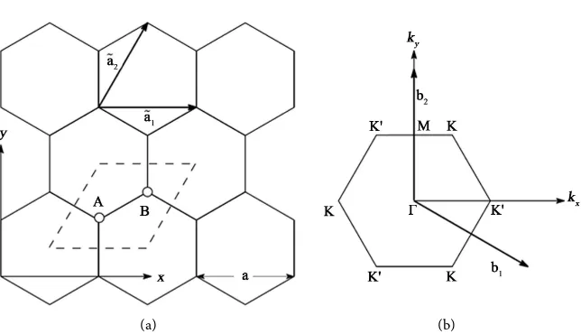
_{is the electron energy. In the semiclassical}

theory electrons are treated as a wave packet. The 2D crystals such as graphene can also be treated similarly, only the z-component being dropped. Graphene forms a 2D honeycomb lattice. The WS unit cell is a rhombus (dotted lines) as shown in Figure 1(a).

The potential energy V r

( )

is lattice-periodic:

(

mn

)

( )

,

V r R+ =V r (4) where Rmn =ma1+na2 are Bravais vectors with the primitive non-orthogonal

vectors

(

a a1, 2

)

and integers

(

m n,

)

. In the field theoretical formulation, the

field point r is given by r r R= +′ mn , where r′ is the point defined within the

[image:3.595.213.535.60.245.2]

(a) (b)

Figure 1. (a) Lattice structure of graphene. Carbon atoms at vertices. Each honeycomb lattice consists of equivalent carbon (C+_{) ions labeled by A and B. The Wigner-Seitz} 2-atom unit cell (dotted lines) spanned by the basis (lattice unit) vectors a1 and a2; (b) Reciprocal lattice showing the first Brillouin zone (BZ) of graphene including the high-symmetry points Γ, K, and M. The BZ is spanned by two reciprocal lattice vectors

1

b and b2 constructed from the basis vectors a1 and a2.

does not establish the k-space for the Bloch electrons in graphene, which will be explained in Section 4, and this fact has motivated us to study the band structure for a Bloch electron based on the rectangular 4-atom unit cell model for graphene (see Figure 2(a)), which defines the k -vectors playing an important roll for a Bloch electron dynamics.

Our purpose of this paper is to explore the suitability of the rectangular (orthogonal) unit cell model for the Bloch electron band structure and to discuss the k-vector defined in the 2D space for Bloch electrons in graphene. Based on the rectangular 4-atom unit cell model of graphene, we obtain the band structure for the 2pz-electrons of graphene by extending the prevalent tight-binding

calculations for the Wigner-Seitz (WS) 2-atom unit cell model to the rectangular (orthogonal) 4-atom unit cell model introduced by the present authors [7].

In Section 2, the rectangular 4-atom unit cell of graphene is introduced. Section 3 presents our tight-binding calculations of the energy band of a Bloch electron in graphene, based on the rectangular 4-atom unit cell model described in Section 2. Section 4 illustrates why we have to utilize the rectangular (orthogonal) unit cell rather than the WS unit cell when considering the electron dynamics of graphene. Results and discussion are given in Section 5. Finally conclusions and some remarks are given in Section 6.

2. The Rectangular 4-Atom Unit Cell Model for Graphene

[image:4.595.212.537.65.245.2]

(a) (b)

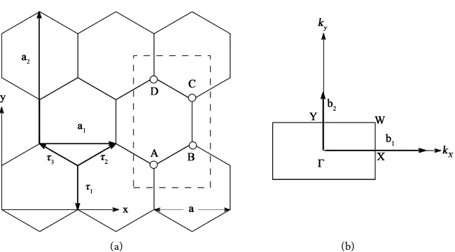
Figure 2. (a) Lattice structure of graphene, made out of the rectangular 4-atom unit cell (a square dotted line) spanned by the basis vectors a1 and a2. The τi

(

i=1,2,3

)

are

the nearest-neighbor vectors with the constant carbon-carbon distance of

3 0.142 nm

i = =

τ a ; (b) The first Brillouin zone of the rectangular 4-atom unit cell. The b1 and b2 are the reciprocal lattice vectors corresponding to the lattice unit vectors. The high-symmetric points within the rectangular unit cell are indicated by Γ, X, Y, and W within the reciprocal lattice plane.

The reason why we choose a rectangular (orthogonal) unit cell rather than a triangular (WS) unit cell for graphene will be explained later.

The lattice basis (unit) vectors ai

(

i=1,2

)

of graphene (cp. Figure 2(a)) are

defined as

( )

( )

1=a 1,0 , 2=a 0, 3 .

a a (5)

The lattice constants for the rectangular (orthogonal) unit cell in the Cartesian coordinates are a1 ≡ =a 3a0 and a2 = 3a=3a0, respectively, where a0

is the nearest-neighbor distance between two carbon atoms. The rectangular 4-atom unit cell of graphene contains four carbon atoms, say A, B, C, and D, as shown in Figure 2(a). The three nearest-neighbor vectors τi

(

i=1, 2,3

)

in real

space are defined (cp. Figure 2(a)) by

(

)

(

)

(

)

1=a 0, 1 3 ,− 2=a 1 2,1 2 3 , 3=a −1 2,1 2 3 .

τ τ τ (6)

The reciprocal-lattice vectors for the rectangular unit cell are given (from Equation (5)) by

( )

(

)

1=2π_a 1,0 , 2 =2π_a 0,1 3 .

b b (7)

The first Brillouin zone is a rectangle as shown in Figure 2(b) with sides of length, BZ

1 2π x

b = b = a and BZ

2 2π 3 y

b = b = a, and area equal to _4π2 _3a2_.

( )

0,0 , X π

( )

1,0 , Y π

(

0,1 3 , W

)

π

(

1,1 3 .

)

a a a

Γ = = = = (8)

3. Tight-Binding Approach

The single-particle band structure of graphene can be analytically calculated within the tight-binding approximation assuming that electrons are tightly bound to their C+ _{ion [8] [9] [10] [11]. In order to obtain the band structure of} graphene based on the 4-atom rectangular unit cell model [7] for graphene, we follow the tight-binding approach employed by Reich et al.[8].

The Schrödinger equation for a single electron in the lattice potential field

( )

V r is expressed by

( )

ε

( )

,

Ψ r = Ψ r

 (9)

where the Hamiltonian  is given by

( )

2

2 _,

2m V

= − ∇ + r

 (10)

and the lattice potential V

( )

r =V

(

r R− j

)

has a lattice periodicity characteristic

for graphene. The total wave function Ψ for the electron in the 2pz-orbital

(Bloch electron) may be obtained from the linear combination of the Bloch wave

j

Φ of the form:

( )

1 j

(

)

,

j

i

j j e j

N φ

⋅

Φ ≡ Φ =

∑

k R −

R

r r r R (11)

where N is the number of unit lattices and the index j refers to the respective carbon atoms. In the above expressions, the phase exp

(

ik R⋅ j

)

are

introduced in order to satisfy the Bloch theorem in each conduction channel. Thus the wave function for a Bloch electron in graphene is then expressed by the linear combinations of these Bloch wave functions:

( )

( )

( )

( )

,

j j j j

j j

λ λ

Ψ ≡ Ψ

=

∑

Φ =

∑

Φ

r r

k r k r (12)

where r Φj ’s are given by Equation (11) and the wave function rφ for

the 2pz-orbital is normalized. The energy eigenvalues of Equation (9) for the 2pz-electron can be obtained in a usual manner by using the graphene Hamil-

tonian (10) and the graphene wave function (12) along with Equation (11): Inserting Equation (12) into Equation (9) and multiplying Φi from the left to

Equation (9), we obtain four separate equations, which are simply expressed in the matrix form as

( )

=ε

( )

; ij jλ

( )

=ε λSij j

( )

,

λ k Sλ k k k

 (13)

where the matrices, , S and λ k

( )

, are respectively expressed by

AA AB AC AD BA BB BC BD CA CB CC CD DA DB DC DD

 

 

 

=

 

 

 

   

   

   

   

AA AB AC AD BA BB BC BD CA CB CC CD DA DB DC DD

S S S S

S S S S

S S S S

S S S S

      =      

S (15)

( )

( )

( )

( )

( )

A B C D . λ λ λ λ       =         k k λ k k k (16)

Here ij ≡ Φi Φj are the matrix elements of the Hamiltonian , which

we call hopping (or transfer) integral, and are the units of energy. Sij ≡ Φ Φi j

are the overlap matrix elements, which are given by the overlap integral between Bloch functions, and are unitless. Equation (13) expresses the simultaneous equations for λA

( )

k , λB

( )

k , λC

( )

k and λD

( )

k . In order to obtain the

nontrivial solutions for λj

( ) (

k A,B,C,Dj=

)

, the secular equation determi-

nant −εS of their simultaneous equations must be zero:

0.

ε

− S=

 (17)

Since the atomic wave functions are well localized around the carbon atoms, only the nearest-neighbor hopping of Bloch electrons are taken into considera- tion of the following calculations. In other words, as for the electron in atom A orbital, it can hop to a nearest orbital of atom B or atom D. Similarly, the electron in the orbital of atom B can hop to the nearest orbital of atom A or atom C, the electron in the orbital of atom C to the nearest orbital of atom B or atom D, and the electron in the orbital of atom D to the nearest orbital of atom A or atom C.

Let us consider the nearest-neighbor hopping between the orbital of atom A and atom B. The matrix elements AB is expressed by the hopping integral:

( B A)

₍

₎

₍

₎

A B

AB A B

A B

1 _ei _.

N φ φ

⋅ −

= Φ Φ

=

∑∑

k R R − −

R R r R r R

 

 (18)

Here we only take into account the nearest-neighbor hopping between carbon atoms. From the symmetry of the lattice stracture of graphene, the adjacent hoppings are all the same. We introduce the parametric parameter t1 for the

adjacent hopping between the orbital of atom A and B:

(

A

)

(

B

)

t1.

φ r R− φ r R− ≡ (19)

Since the nearest-neighbor vector R RB− A is given by τ2 and τ3 (cp.

Equation (6)), Equation (18) can be expressed by

( )

₍

₎

₍

₎

(

)

B A A B 3 2

AB A B

2 3

1 1

1

2 cos .

2 y i a i k i i x e N a

t e e t e k

φ φ ⋅ − − ⋅ − ⋅ = − −   ≈ + = _{ }  

∑∑

k R R

R R

k τ k τ

r R r R

 

(20)

3 3 AC AD 1 BC 1

2 3 BD CD 1

0, , ,

0, 2 cos .

2

y y

y

a a

i k i k

a i k

x

t e t e

a

t e k

− = = =   = = _{ }        (21)

We note that the hopping parameter t1 is the nearest-neighbor hopping energy

(hopping between adjacent carbon atoms).

The matrix element AA (on-site hopping) is evaluated as

( )

₍

₎

₍

₎

(

)

(

)

A A A A

A

AA A A

A A A A 0 1 1 , i e N N t φ φ φ φ ′ ′ ⋅ − ′

= Φ Φ

= − −

≈ − −

≡

∑ ∑

∑

k R R

R R

R

r R r R

r R r R









(22)

where N is the number of the basic unit cells, and t0 is the parametric

parameter for φ

(

r R− A

)

φ

(

r R− A

)

. Similar evaluation leads to

BB= CC = DD=t0

   .

Next we evaluate the matrix elements S i jij

(

, =A,B,C,D

)

, which are given by

the overlap integral Φ Φi j . Thus the matrix element SAB is evaluated from

( B A)

₍

_{) (}

₎

A B

AB A B

A B

1 i _.

S

e

N φ φ

⋅ −

= Φ Φ

=

∑∑

k R R − −

R R r R r R

(23)

Introducing the parametric parameter s1 for the overlap integral:

(

A

) (

B

)

s1,

φ r R− φ r R− ≡ (24)

the matrix element SAB is given by

2 3

AB 21 cos ₂ .

y

a i k

x

a

S = s e _ k _

  (25)

Similarly we obtain

3 3

AC AD 1 BC 1

2 3 BD CD 1

0, , ,

0, 2 cos .

2

y y

y

a a

i k i k

a i k

x

S S s e S s e

a

S S s e k

− = = =   = = _{ }   (26)

We note that the matrix element SAA is evaluated as

( )

₍

_{) (}

₎

(

) (

)

A A A A

A

AA A A

A A A A 1 1 1. ik S e N N φ φ φ φ ′ ′ ⋅ − ′

= Φ Φ

= − − ≈ − − =

∑ ∑

∑

R R R R R

r R r R

r R r R

(27)

In a similar manner, we obtain

BB CC DD 1.

We can solve Equation (17) for

ε

_{by using Equations (18)-(28) for the}

matrix elements, and obtain the four energy eigenvalues of Equation (9) for the graphene π-electron bands:

2 0 1 c 2 1 3

1 4_{cos 2} 4cos cos

2 2

, 3

1 1 4_{cos 2} 4cos cos

2 2

x y x

x y x

a a a

t t k k k

a a a

s k k k

ε       − + _ _± _ _ _ _   =       − + _{ }± _{   }   _{ }   (29) 2 0 1 v 2 1 3

1 4_{cos 2} 4cos cos

2 2

, 3

1 1 4_{cos 2} 4cos cos

2 2

x y x

x y x

a a a

t t k k k

a a a

s k k k

ε       + +  ± _ _     _{ }   =       + + _ _± _ _ _ _   (30)

where εc and εv are the conduction-and the valence-band energies, respec-

tively.

4. Electron Dynamics of Graphene

In semiclassical (wave packet) theory for electron dynamics, it is necessary to introduce a wave vector k (namely, k-vector) [6] [12] since the k-vectors are involved in the semiclassical equation of motion (see Equation (2)). Here, we explain why we employed the rectangular (orthogonal) unit cell for graphene in order to calculate one electron energy band for graphene.

Graphene forms a 2D honeycomb lattice. Let us first consider the Wigner- Seitz (WS) unit cell (rhombus, dotted lines shown in Figure 1(a)). The potential energy V r

( )

is lattice-periodic:

(

)

( )

,

V r R+ =V r (31) where the position vector R in the potential field V can be represented by Bravais vectors with the primitive (non-orthogonal) basis vectors

(

a a1, 2

)

and

integers

(

m n,

)

:

1 2.

mn m n

≡ = +

R R a a (32)

In the field theoretical formulation, the field point r is given by

, mn ′ = +

r r R (33) where r′ is the point defined within the standard WS unit cell. Equation (31) describes the (2D) lattice periodicity but does not establish the 2D k-vector of a Bloch electron in graphene if we choose the non-Cartesian coordinates system. Thus the WS unit cell is not appropriate when one deals with graphene transport problem, which is explained below.

We assume that the wave packet is composed of superposable plane-waves characterized by the k-vectors. The superposability is the basic property of the Schrödinger wave equation. The Schrödinger wave equation for a Bloch electron (wave packet) is

( )

2 2

( )

( ) ( )

* ,

2

i V

t ψ m ψ ψ

∂

= − ∇ +

∂

r r r r (34)

lattice, Rmn, are given by Equation (32) and the system is lattice-periodic, cp.

Equation (31). The Bloch theorem can be expressed in the form:

( )

, _ei

(

)

ψ ₌ ψ ₌ k R⋅ ψ ₋

k r r k k r R (35)

for all R in the Bravais lattice. The theorem in 1D can be proved elementarily

[6]. If an oblique lattice is considered and a set of nonorthogonal basis vectors

(

a a1, 2

)

are introduced for a 2D Bravais vector, cp. Equation (32), there are no

2D Fourier transform available since there is no 2D k-vector to satisfy the periodicity condition for the Bloch wave, which must be of the form (35). Thus, the WS unit cell model for graphene is not suitable when one considers the electron dynamics in graphene.

The wave function must be Fourier-analyzable. In the rhombic system, however, if we choose the x-axis, say along a1, then the potential energy field

( )

V r is periodic in the x-direction, but it is aperiodic in the y-direction (cp.

Figure 1(a)) since these basis vectors

(

a a1, 2

)

are not orthogonal each other.

Thus, if we choose the rhombic unit cell for graphene, we cannot express k- vectors satisfying the condition for the Bloch wave (35). Then, there is no 2D k

space spanned by 2D k-vectors of Bloch waves if we choose the rhombic unit cell. If we omit the kinetic energy term, then we can still use Equation (31) and obtain the ground state energy (except the zero-point energy).

Ashcroft and Mermin (AM) [6] introduced a translation operator R such

that acting on any field f r

( )

it shifts its argument by R:

( )

(

)

.

f = f +

R r r R

 (36)

They used

=

R R

   (37)

to establish Equation (35). The translation operator X can be expressed in

terms of a differential operator:

exp

X X _x

∂

 

= _{ }

∂

 

 (38)

as seen from exp X f x

( )

f x X

(

)

x

∂

  _{= +}

 _∂ 

  . If the Bravais vector R is given in

terms of the orthogonal basis vectors

(

a a1, 2

)

in the Cartesian coordinates and

choose the rectangular unit cell (cp. Figure 2(a)) as in Equation (34), then Equation (37) is satisfied, meaning that the Bloch wave for a rectangular unit cell can be expressed in terms of the Bloch wave (35).

If R is written in terms of nonorthogonal

(

a a1, 2

)

, then R is a product

of differential operators exp X x ∂

 

 _∂ 

  and exp Y y  ∂   _∂ 

  , which does not

commute with the Laplacian 2 2 2

2 2

x y

 ∂ ∂ 

∇ =_ + _

∂ ∂

  in the Hamiltonian operator

is valid for the Bloch wave (35), where the Bravais vectors are expressed by the orthogonal basis vectors in the Cartesian coordinates. It should be noted that for an infinite lattice the periodic boundary is the only acceptable boundary condition for the Fourier transformation. AM’s second proof [6] also fails in 2D if the Bravais vector R is expressed in nonorthogonal base vectors. This is so because Laplacian terms cannot be handled in non-Cartesian (oblique) coordinates. AM's Equation (8.36) does not hold. We must choose the rectangular unit cell in order to establish the Bloch plane waves [13] [14] for the “electron” in 2D.

We assume that the “electron” (“hole”') (wave packet) has the charge

( )

e e

− + _{and a size of the rectangular unit cell, generated above (below) the} Fermi energy εF. It was shown [7] [15] that (a) the “electron” and the “hole”

have different charge distribution and different effective masses, (b) that the “electron” and “hole” move in different easy channels, (c) that the “electrons” and “holes” are thermally excited with different activation energies, and (d) that the “electron” activation energy ε1 is smaller than the “hole” activation energy

2

ε _:

1 2

ε <ε ₍₃₉₎

Thus, “electrons” are the majority carriers in graphene. The thermally activated electron densities are then given by

( )

exp

(

) (

, constant ,

)

i i i B i

n T =n −ε k T n = (40)

where i=1 and 2 represent the “electron” and “hole”, respectively. The pre- factor ni is the density at the high-temperature limit. Magnetotransport ex-

periments by Zhang et al. [16] indicate that the “electrons” are the majority carriers in graphene. Thus, our theory based on the rectangular unit cell model is agreement with experiments.

At finite temperature phonons are present in the system. The excitation of phonons can be discussed based on the same rectangular unit cell introduced for the conduction electrons. We note that phonons can be discussed naturally based on the orthogonal unit cells. It is difficult to describe phonons in the WS cell model.

5. Results and Discussion

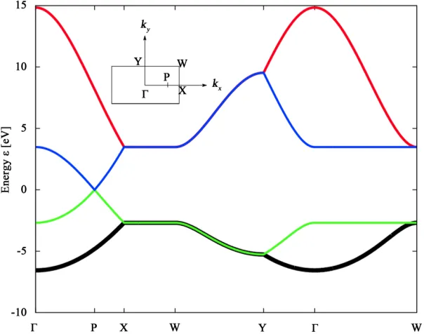
Based on the rectangular 4-atom unit cell model, we obtained the band disper- sion of graphene by applying the tight-binding theory of Reich et al. [8]. The obtained (π-) band structure based on the rectangular 4-atom unit cell model for graphene computed from Equations (29) and (30) is shown in Figure 3, where the nearest-neighbor hopping parameters t1 and s1 are taken from the

values obtained by the ab initio calculation [8] [17]: t0 =0 eV, t1= −3.033 eV, 1 0.129

s = _{. This 3D figure illustrates the conduction and the valence band}

within the first Brillouin zone. The two crossing points P and Q indicated in the figure are of particular importance for the physics of graphene.

[image:11.595.251.496.69.322.2]

Figure 3. (Color online) Band structure of graphene based on the rectangular 4-atom unit cell model. The energy is maximal at the Γ-point in the conduction band, while there is a saddle-point at the Γ-point in the valence band in the first BZ. The display shows the linear dispersion structure around the crossing-points P and Q, at which

( )

0 ε± _{k = .}

[image:11.595.223.525.413.651.2]

space. There are two crossing points P and Q in the first BZ (cp. Figure 3), at which the band energy is crossing (i.e., ε±

( )

P ₌ε±

( )

Q ₌0_{), suggesting that} graphene is a zero gap semiconductor.

Let us take a close look at the behavior of the band energy close to the crossing points, at which the band energy equals to zero. The conduction and valence bands are degenerate at this point. The dispersion relation for small momenta

k near the crossing points P 2

(

π3 ,0a

)

and Q 2

(

− π3 ,0a

)

_{is given by Taylor}

expanding the band energy around the points P and Q, resulting in a unique

linear energy dispersion:

( )

2 2

F F x y F ,

v v k k v k

ε± _{k = ± k = ± + = ± (41)}

where k

(

= k

)

is now in spherical coordinates (their origin is now at the points P and Q), vF the Fermi velocity given by vF≈

(

3 2

)

at1=0.98 10 m s× 6 ⋅ −1

with a= a1 =0.246 nm, t1= −3.033 eV. This particular band structure re-

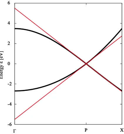
[image:12.595.268.479.423.651.2]

sembles the physics of massless Dirac fermions with a velocity approximately 300 times smaller than the speed of light. Near the crossing point P in the first Brillouin zone, the linear dispersion (Equation (41)) is clearly seen in the plot in

Figure 5 for the rectangular 4-atom unit cell model for graphene. The linear dispersion for small k also holds for the crossing point Q as well.

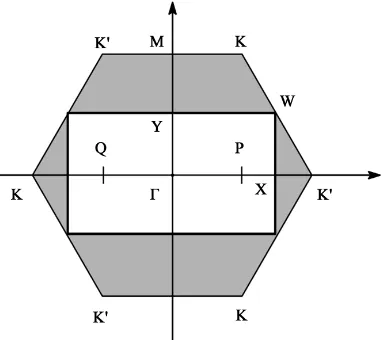
The second BZ of the reciprocal lattice for the rectangular 4-atom unit cell is shown by the shaded area in Figure 6. The high symmetric points in the reciprocal lattice of the rectangular 4-atom unit cell are indicated by Γ, X, Y,

[image:13.595.278.469.71.241.2]

Figure 6. The first Brillouin zone (rectangular) and the second Brillouin (shaded) zone of the rectangular 4-atom unit cell. The region of the first and second BZ’s (i.e., the hexagonal region) of the rectangular 4-atom unit cell is identical to the first BZ of the Wigner-Seitz 2-atom unit cell.

and W, while those in the reciprocal lattice of the 2-atom unit cell are indicated by Γ, M and K. The Dirac points of the Wigner-Seitz 2-atom unit cell are indicated by K and K’ in Figure 6, while the crossing (so-called Dirac) points of the first BZ of the 4-atom unit cell are located at the points P, Q in the first BZ of the 4-atom unit cell. Note that the first Brillouin zone of the Wigner-Seitz 2-atom unit cell is identical to the region of the first and second Brillouin zone of the rectangular 4-atom unit cell (hexagon. cp. Figure 6). The crossing points, P and Q, in the first Brillouin zone of the rectangular 4-atom unit cell correspond to the Dirac points, K and K’ of the Wigner-Seitz 2-atom unit cell since the energy band structure of the rectangular 4-atom unit cell model is identical to the folded band structure of the 2-atom unit cell model along the boundary of the first BZ of the 4-atom unit cell model.

The approximate results (π-bands) obtained in this paper are based on the rectangular 4-atom unit cell model for graphene by using tight-binding calculations, where only the nearest-neighbor hopping is taken into account for the transport of Bloch electrons. The horizontal ε

( )

k =0 line shows the chemical potential. Below the chemical potential, the states are all occupied and the conduction states are above it. The chemical potential is at the points labeled P and Q in the first BZ, where the valence and conduction bands are crossing. The bands with the lowest energy are from the

σ

-bands in the planes between the carbon atoms. Electrons in the

σ

_{-bands are tightly bound. The energy}

bands near the chemical potential are from the π-bands. They are formed from the carbon orbital pz, which projects above and below the plane of graphene.

These π-bands are well described by a nearest-neighbor tight-binding calcula- tions based on the 4-atom unit cell model.

6. Conclusions and Some Remarks

[7]. Based on this model, we obtained the band energy by applying the tight- binding approach employed by Reich et al. [8]. We proved the band structure based on the rectangular 4-atom unit cell model for graphene gives the same band structure of graphene based on the prevalent graphene model based on the Wigner-Seitz 2-atom unit cell model.

The rectangular 4-atom unit cell for graphene has the sides perpendicular to each other (see Figure 2). The k-vector k is defined as in Equation (1) but with the orthogonal unit vector, and the k is obtained as the Fourier conjugate of the position vector r.

The transport electrons in graphene originating from the π-band can be described by the 2D Bloch k-vector defined in the proposed rectangular unit cell. We showed that the energy dispersion relation near the Dirac points (small

k) shows the linear dependence of k (see Equation (41)).

A material (density) wave such as a phonon wave can be presented by a traveling wave function of the form: Cexp

(

−i t iω + ⋅k r

)

with C _{= material}

density,

ω

= angular frequency, and k=k -vector. The direction of k

points to the direction of the traveling plane wave.

In the currently prevailing theory [2] [3] [4] [5] [8] [9] [10] [11] [17] the solid state theory dealing with a hexagonal crystal starts with a primitive non- orthogonal unit cell, the 2-atom unit cell. This theoretical model has difficulties in particular for a superconductor. The ground state of a superconductor must be condensed in a single particle-state in accordance with Nernst’s theorem (the third law of thermodynamics). Many fermions have a distribution in energy and hence a many-fermion system cannot be a superconductor. Only many-boson system can be a superconductor.

In the prevailing theory [2] [3] [4] [5] [8] [9] [10] [11] [17] a 2-atom unit cell model is used to set up k-vectors with non-orthogonal unit vectors a1 and

2

a . A Bloch k -vector is k=k1 1a +k2 2a constructed with the Born-von

Karman boundary condition [6]. But this vector is not useful in dealing with a superconducting intercalation graphite compound.

In the present work we have shown that the non-orthogonal 2-atom and orthogonal 4-atom models give the same band energies in the mean field appro- ximation. In separate publication we report the superconductivity in graphite intercalation compounds C8K, C6Ca and in compound MgB2.

References

[1] Geim, A.K. and Noboselov, K.S. (2007) Nature Materials, 6, 183-191. https://doi.org/10.1038/nmat1849

[2] Neto, A.H.C., Guinea, F., Peres, N.M.R., Novoselov, K.S. and Geim, A.K. (2009) Re-views of Modern Physics, 81, 109. https://doi.org/10.1103/RevModPhys.81.109 [3] Sarma, S.D., Adam, S., Hwang, E. and Rossi, E. (2011) Reviews of Modern Physics,

83, 407. https://doi.org/10.1103/RevModPhys.83.407

[5] Reich, S., Thomsen, C. and Maultzsch, J. (2004) Carbon Nanotubes: Basic Concepts and Physical Properties. Wiley-VCH Verlag GmbH, Berlin.

[6] Ashcroft, N.W. and Mermin, N.D. (1976) Solid State Physics. Saunders, Philadel-phia, 75, 133-135, 137-139, 228-229.

[7] Fujita, S. and Suzuki, A. (2010) Journal of Applied Physics, 107, Article ID: 013711. https://doi.org/10.1063/1.3280035

[8] Reich, S., Maultzsch, J., Thomsen, C. and Ordejön, P. (2002) Physical Review B, 66, Article ID: 035412. https://doi.org/10.1103/PhysRevB.66.035412

[9] Wallace, P.R. (1947) Physical Review, 71, 622. https://doi.org/10.1103/PhysRev.71.622

[10] McClure, J.W. (1957) Physical Review, 108, 612. https://doi.org/10.1103/PhysRev.108.612

[11] Slonczewski, J.S. and Weiss, P.R. (1958) Physical Review, 109, 272. https://doi.org/10.1103/PhysRev.109.272

[12] Fujita, S. and Ito, K. (2007) Quantum Theory of Conducting Matter: Newtonian Equations of Motion for a Bloch Electron. Springer, New York, 120-121, 192-193. https://doi.org/10.1007/978-0-387-74103-1

[13] Bloch, F. (1929) Zeitschrift für Physik, 52, 555-600. https://doi.org/10.1007/BF01339455

[14] Fujita, S., Jovaini, A., Godoy, S. and Suzuki, A. (2012) Physics Letters A, 376, 2808- 2811.

[15] Fujita, S., Takato, Y. and Suzuki, A. (2011)Modern Physics Letters B, 25, 223. https://doi.org/10.1142/S0217984911025675

[16] Zhang, Y., Tan, Y.W., Stormer, H.L. and Kim, P. (2005) Nature, 438, 201-204. https://doi.org/10.1038/nature04235

[17] Saito, R., Dresselhaus, G. and Dresselhaus, M.S. (2005) Physical Properties of Car-bon Nanotubes. Imperial College Press, London.

Submit or recommend next manuscript to SCIRP and we will provide best service for you:

Accepting pre-submission inquiries through Email, Facebook, LinkedIn, Twitter, etc. A wide selection of journals (inclusive of 9 subjects, more than 200 journals)

Providing 24-hour high-quality service User-friendly online submission system Fair and swift peer-review system

Efficient typesetting and proofreading procedure

Display of the result of downloads and visits, as well as the number of cited articles Maximum dissemination of your research work

Submit your manuscript at: http://papersubmission.scirp.org/