Munich Personal RePEc Archive
The k-NN algorithm for compositional
data: a revised approach with and
without zero values present
Tsagris, Michail
University of Nottingham
July 2014
Online at
https://mpra.ub.uni-muenchen.de/65866/
The
k
-NN algorithm for compositional data: a revised approach
with and without zero values present
Michail Tsagris
School of Mathematical Sciences, University of Nottingham, UK [email protected],
Abstract
In compositional data, an observation is a vector with non-negative components which sum to a constant, typically 1. Data of this type arise in many areas, such as geology, archaeology, biology, economics and political science among others. The goal of this paper is to extend the taxicab metric and a newly suggested metric for compositional data by employing a power
transformation. Both metrics are to be used in thek-nearest neighbours algorithm regardless
of the presence of zeros. Examples with real data are exhibited.
Keywords: compositional data, entropy,k-NN algorithm, metric, supervised classification
1
Introduction
Compositional data are non-negative multivariate data and each vector sums to the same constant, usually 1 for convenience. Compositional data are met in many disciplines, includ-ing geology (Aitchison, 1982), economics (Fry et al., 2000), archaeology (Baxter et al., 2005)
and political sciences (Rodriques and Lima, 2009). Their sample space is called simplex Sd
and in mathematical terms is
Sd=
(
(x1, ..., xD)T
xi≥0, D
X
i=1
xi= 1
)
,
where D denotes the number of components andd =D−1.
Ever since Aitchison (1982) suggested the use of the log-ratio transformation for composi-tional data, most of the analyses of such data have been implemented using this transforma-tion. Aitchison (2003) implemented linear discriminant analysis for compositional data using the log-ratio transformation. Over the years though, researchers have suggested alternative ways for supervised classification of compositional data, see for example Gallo (2010) and Neocleous et al. (2011).
An important issue in compositional data is the presence of zeros, which cause problems for the logarithmic transformation. The issue of zero values in some components is not addressed in most papers, but see Neocleous et al. (2011) for an example of discrimination in the presence of zeros. Alternatively, one could use alternative models (see for example Scealy and Welsh, 2011a and Stewart and Field, 2011) or replace the zero values by making parametric assumptions (Martin et al., 2012).
In this paper we suggest the use of a recently developed metric, for classification of
a metric for probability distributions (Endres and Schindelin, 2003; ¨Osterreicher and Vajda, 2003) which can be adopted to compositional data as well, since each vector sums to 1. The second metric we suggest is the Manhattan metric, a scaled version of which has already been used for compositional data analysis (Miller, 2002). We will extend both of these metrics by applying a power transformation. We will see that both of these metrics handle zeros naturally and hence they can be used regardless of them being present in some components. This is a very attractive feature of these metrics in contrast to the Aitchisonian metric suggested by Aitchison (2003) which is not applicable when zeros are present in the data. Examples using real data are used to illustrate the performance of these metrics.
Section 2 describes the two metrics, how they can be extended and also presents
graphi-cally their loci of points equidistant from the centre of the simplex. Section 3 shows thek-NN
algorithm for compositional data and Section 4 contains examples using real data. Finally, section 5 concludes this paper.
2
Metrics for compositional data
We will present three metrics for compositional data ,two of which have already been exam-ined. But first we will show the power transformation. Aitchison (2003) defined the power transformation to be
u= x
α 1
PD
j=1xαj
, . . . , x
α D
PD
j=1xαj
!T
. (1)
The value of α will be determined by the estimated accuracy of thek-NN algorithm.
2.1
The ES-OV
αmetric for compositional data
We advocate that as a measure of the distance between two compositions we can use the square root of the Jensen-Shannon divergence
ES−OV(x,w) =
"D
X
i=1
xilog 2
xi
xi+wi
+wilog 2
wi
xi+wi
#1/2
, (2)
where x,w∈Sd.
Endres and Schindelin (2003) and ¨Osterreicher and Vajda (2003) proved, independently,
that (2) satisfies the triangular identity and thus it is a metric. For this reason we will refer to it as the ES-OV metric.
We will use the power transformation (1) to define a more general metric termed ES-OVα
metric
ES−OVα(x,w) =
D X i=1
xαi
PD
j=1xαj
log
2Pxαi
D j=1xαj xα
i
PD
j=1xαj
+Pwαi
D j=1wαj
+ w
α i
PD
j=1wjα
log
2Pwiα
D j=1wαj xα
i
PD
j=1xαj
+Pwiα
D j=1wαj
1/2
2.2
The taxicab
αmetric for compositional data
The taxicab metric is also known asL1 (or Manhattan) metric and is defined as
T C(x,w) =
D
X
i=1
|xi−wi| (4)
We will again employ the power transformation (1) to define a more general metric which
we will term the TCα metric
T Cα(x,w) = D
X
i=1
xα i
PD
j=1x α j
− w α i
PD
j=1w α j
(5)
2.3
The Aitchisonian metric for compositional data
Aitchison (2003) suggested the Euclidean metric applied to the log-ratio transformed data as a measure of distance between compositions
Ait(x,w) =
"D
X
i=1
log xi
g(x)−log wi
g(w)
2#1/2
, (6)
where g(z) =QD
i=1z
1/D
i stands for the geometric mean.
2.4
Some comments
The power transformed compositional vectors still sum to 1 and thus the ES-OVα (3) is still
a metric. It becomes clear that whenα = 1 we end up with the ES-OV metric (2). If on the
other hand α = 0, then the distance is zero, since the compositional vectors become equal
to the centre of the simplex. An advantage of the ES-OVα metric (3) over the Aitchisonian
metric (6) is that the the first one is defined even when zero values are present. In this case the Aitchisonian metric (6) becomes degenerate and thus cannot be used. We have to note that we need to scale the data so that they sum to 1 in the case of the ES-OV metric, but this is not a requirement of the taxicab metric.
Alternative metrics could be used as well, such as
1. the Hellinger metric (Owen, 2001)
H(x,w) = √1
2
"D
X
i=1
(√xi−√wi)2
#1/2
2. or the angular metric if we treat compositional data as directional data (for more information about this approach see Stephens (1982) and Scealy and Welsh (2011, 2014))
Ang(x,w) = arccos
D
X
i=1
xiwi
Aitchison (1992) argued that a simplicial metric should satisfy certain properties. These properties include
1. Scale invariance. The requirement here is that the measure used to define the distance between two compositional data vectors should be scale invariant, in the sense that it makes no difference whether the compositions are represented by proportions or percentages.
2. Subcompositional dominance. To explain this we consider two compositional data vec-tors and we select sub-vecvec-tors from each consisting of the same components. Subcom-positional dominance means that the distance between the sub-vectors is always less than or equal to the distance between the original compositional vectors.
3. Perturbation invariance. The requirement here is that the distance between
composi-tional vectors x and w should be the same as distance between x⊕0p and w⊕0 p,
where the operator ⊕0 means element-wise multiplication and then division by the
sum so that the resulting vectors belong to Sd and p is any vector (not necessarily
compositional) with positive components.
If all of the above metrics satisfy or not these thee properties should not be a problem. Take for example subcompositional dominance. If someone has a compositional dataset, there has to be a good reason why he would choose to discard some components and form a sub-composition. And even if he does, all the metrics are still applicable.
The message this paper tries to convey is that if someone uses a well defined metric (or even a dissimilarity measure) in order to perform classification he should be fine with that. When dealing with data lying on the Euclidean space, one can use dissimilarity measures as well to perform clustering or discrimination. The question of interest is how can we discriminate the observed groups of points as adequately as possible.
2.5
Loci of points equidistant from the centre of the simplex
Figure 1 shows the effect of the power transformation (1) on the data. As expected, the data
come closer to the barycentre of the triangle asα tends to zero. The data used and plotted
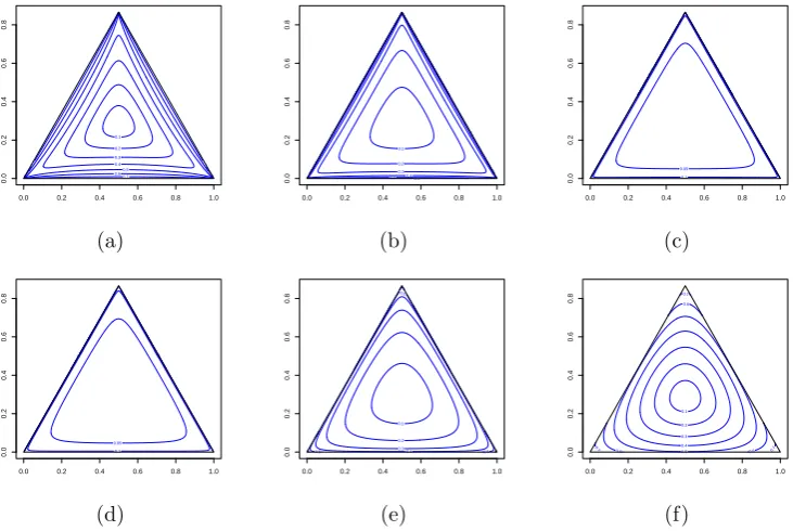
on Figure 1 are the Arctic lake data (Aitchison, 2003). Figures 2 and 3 show the plots of
loci of points of the ES-OVα metric (3) and of the TCα metric (5) for different values of α
and Figure 4 shows the contour plots of the Aitchisonian metric (6). In all cases, the plots of loci of points refer to the distance from the barycentre of the simplex. The loci of points
seen on Figure 2 have similar shape regardless of the value ofα. This is not true for the loci
sand silt clay sand silt clay sand silt clay
(a) (b) (c)
sand silt clay sand silt clay sand silt clay
[image:6.595.119.485.86.331.2](d) (e) (f)
Figure 1: Ternary plots of the Arctic lake data (Aitchison, 2003) for different values of α.
The data are transformed calculated using (a) α = −1, (b) α = −0.5, (c) α = −0.1, (d)
α= 0.1, (e) α= 0.5 and (f) α = 1.
0.1 0.2 0.3 0.4 0.5
0.6 0.7 0.6 0.6
0.7
0.7
0.0 0.2 0.4 0.6 0.8 1.0
0.0 0.2 0.4 0.6 0.8 0.1 0.2 0.3 0.4
0.5 0.5
0.5
0.6
0.6
0.6
0.0 0.2 0.4 0.6 0.8 1.0
0.0 0.2 0.4 0.6 0.8 0.05 0.1 0.15 0.15
0.0 0.2 0.4 0.6 0.8 1.0
0.0
0.2
0.4
0.6
0.8
(a) (b) (c)
0.05 0.1
0.15
0.15
0.0 0.2 0.4 0.6 0.8 1.0
0.0 0.2 0.4 0.6 0.8 0.1 0.2 0.3 0.4 0.5 0.5 0.5
0.0 0.2 0.4 0.6 0.8 1.0
0.0 0.2 0.4 0.6 0.8 0.1 0.2 0.3 0.4 0.5 0.6 0.6 0.6 0.7 0.7 0.7
0.0 0.2 0.4 0.6 0.8 1.0
0.0
0.2
0.4
0.6
0.8
(d) (e) (f)
Figure 2: Loci of points equidistant from the centre of the simplex using the ESOVα metric
(3). In all cases the distances are from the barycentre of the simplex (1/3,1/3,1/3). The
contours are calculated using (a) α = −1, (b) α = −0.5, (c) α = −0.1, (d) α = 0.1, (e)
[image:6.595.116.482.404.649.2]0.1 0.2 0.3 0.4 0.5 0.6 0.7 0.7 0.8
0.8 0.8
0.9 0.9
0.9 1 1 1 1.1 1.1 1.1 1.2 1.2 1.2 1.3 1.3 1.3
0.0 0.2 0.4 0.6 0.8 1.0
0.0 0.2 0.4 0.6 0.8 0.1 0.2 0.3 0.4 0.5 0.6
0.7 0.8 0.7 0.7
0.8 0.8 0.9 0.9 0.9 1 1 1 1.1 1.1 1.1 1.2 1.2
0.0 0.2 0.4 0.6 0.8 1.0
0.0 0.2 0.4 0.6 0.8 0.1 0.2 0.3 0.3
0.0 0.2 0.4 0.6 0.8 1.0
0.0
0.2
0.4
0.6
0.8
(a) (b) (c)
0.05 0.1 0.15 0.2
0.25
0.25
0.0 0.2 0.4 0.6 0.8 1.0
0.0 0.2 0.4 0.6 0.8 0.1 0.2 0.3 0.4 0.5 0.6 0.7 0.7 0.7
0.8 0.8
0.9
0.9
0.9
0.0 0.2 0.4 0.6 0.8 1.0
0.0 0.2 0.4 0.6 0.8 0.1 0.2 0.3 0.4 0.5 0.6 0.7 0.7 0.7 0.8 0.8 0.8 0.9 0.9 0.9 1 1 1 1.1 1.1 1.1 1.2 1.2 1.2
0.0 0.2 0.4 0.6 0.8 1.0
0.0
0.2
0.4
0.6
0.8
[image:7.595.115.483.77.323.2](d) (e) (f)
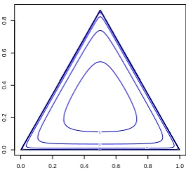
Figure 3: Loci of points equidistant from the centre of the simplex using the TCα metric (5).
In all cases the distances are from the barycentre of the simplex (1/3,1/3,1/3). The contours
are calculated using (a) α =−1, (b) α = −0.5, (c) α =−0.1, (d) α = 0.1, (e) α = 0.5 and
(f) α= 1.
1
2 3 4
5
0.0 0.2 0.4 0.6 0.8 1.0
0.0
0.2
0.4
0.6
0.8
Figure 4: Loci of points equidistant from the centre of the simplex using the Aitchisonian metric (6).
3
Supervised classification for compositional data
us-ing the
k
-NN algorithm
The goal of this paper is to perform supervised classification of compositional data using
the k-NN algorithm. For this reason we will use the ES-OVα (3) and TCα (5) metrics and
compare their performance and suitability with the Aitchisonian metric metric (6).
The k-NN algorithm is a non-parametric supervised learning technique which is
compu-tationally heavier than quadratic and linear discriminant analysis but easier to implement as it relies solely on metrics between points.
[image:7.595.231.364.413.536.2]The two parameters associated with it in our case are the power parameterαand the number
of nearest neighbours k. We describe the steps of the k-NN for compositional data in our
case.
1. Separate the data into the training and the test dataset.
2. Choose a value ofk, the number of nearest neighbours.
3. Classify the test data using either the ES-OVα (3), the TCα (5) for a range of values
of α and each time calculate the percentage of correct classification.
4. Repeat steps 2−3 for a different value of k.
5. Repeat steps 1−4 B (in our case B = 200) times and for each α and k and estimate
the percentage of correct classification by averaging over all B times.
We can of course use the Aitchisonian metric (6) instead of the ES-OVα (3) or the TCα
metric (5). In this case we have to choose the number of nearest neighbours only, since no
power transformation is involved. We could of course use any other metric defined inRd. In
this case we would have to apply the additive log-ratio transformation (Aitchison, 2003) to the data. The issue in that case though would be the presence of zeros in the data.
In the next section we will see two examples using real data and see the performance of the algorithm when each of the two metrics is used.
3.1
Examples using real data
We will now see the performance of the k-NN algorithm using the ES-OVα metric (3), the
TCα metric and the Aitchisonian metric (6) with real data.
Example 1. Hydrochemical data with no zero values
The first dataset comes from hydrochemistry. A hydrochemical data set (Otero et al., 2005) contains measurements on 14 elements. the data were gathered within a period of 2 years from 31 stations located along the rivers and main tributaries of the Llobregat river, one of the medium rivers in northeastern Spain. Each of these elements is measured approximately once each month during these 2 years. There are 4 tributaries of interest, Anoia (143 mea-surements), Cardener (95 meamea-surements), Upper Llobregat (135 measurements) and Lower Llobregat (112 measurements). Thus, there are 485 across all 4 tributaries.
This dataset contains no zero values, so all three metrics are applicable. The size of the training sample was equal to 434 and thus the test sample consisted of 51 observations, which were sampled using stratified random sampling each time to ensure that observations from all tributaries are selected every time. Figure 5 shows the heat plot of the estimated percentage
for different values ofk and α.
Ifα= 0.5 and k= 2 the estimated percentage percentage of correct classification is equal
−1.0 −0.5 0.0 0.5 1.0
2
4
6
8
10
α values
k (n
umber of nearest neighbours)
0.55 0.60 0.65 0.70 0.75 0.80 0.85 0.90
−1.0 −0.5 0.0 0.5 1.0
2
4
6
8
10
α values
k (n
umber of nearest neighbours)
0.5 0.6 0.7 0.8 0.9
[image:9.595.95.494.85.269.2](a) (b)
Figure 5: The estimated percentage of correct classification for the hydrochemical data as a
function ofk, the nearest neighbours and of α using the (a) ES-OVα metric (3) and (b) TCα
(5).
2 4 6 8 10
0.80
0.85
0.90
0.95
2 4 6 8 10
0.80
0.85
0.90
0.95
2 4 6 8 10
0.80
0.85
0.90
0.95
2 4 6 8 10
0.80
0.85
0.90
0.95
2 4 6 8 10
0.80
0.85
0.90
0.95
k (number of nearest neighbours)
Estimated percentage of correct classification
Figure 6: The estimated percentage of correct classification as a function of k. The black
and the red lines are based on the ES-OVα metric (3) with α = 0.5 and α = 1 respectively.
The green and the blue lines are based on the TCα metric (5) with α = 0.35 and α = 1
respectively. The turquoise line is the Aitchisonian metric (6).
metric (3) was applied. When the TCα metric (5) is applied the results are similar, with
α = 0.35 and k = 2 the estimated percentage of correct classification is 93.77% and when
α = 1 and k = 2, the estimated percentage of correct classification is 86.55%. This is an
example where a value ofαother than 1 leads to better results. The change in the percentage
might seem small, but if we take into account the total sample size, we will see that the 3% of 485 observations is 14 observations and it is not a small number. The Aitchisonian metric on the other hand did not do that well. The maximum estimated percentage was equal to
85.46% when k = 2.
[image:9.595.199.382.347.515.2]general conclusion about the mean sensitivities and specificities is that the lower sensitivities are observed when the estimated percentage of correct classification is lower and they have also larger standard errors. The mean specificities on the other hand are in general high and are less affected by the estimated percentage of correct classification.
ES-OVα metric
Tuning parameters Percentage of Tributaries Sensitivities Specificities
correct classification
α= 0.5 & k=2 92.78% (3.25%) Anoia 95.77%(4.92%) 98.60%(2.14%)
Cardener 85.25%(10.65%) 97.06%(2.32%)
Upper Llobregat 93.93%(6.07%) 97.58%(2.34%)
Lower Llobregat 94.00%(6.48%) 97.24%(2.37%)
α= 1 & k=3 89.88% (3.96%) Anoia 93.57%(5.92%) 97.17%(2.83%)
Cardener 82.10%(12.82%) 96.13%(2.83%)
Upper Llobregat 91.50%(7.42%) 96.42%(2.84%)
Lower Llobregat 89.88%(8.39%) 96.85%(2.63%)
TCα metric
Tuning parameters Percentage of Tributaries Sensitivities Specificities
correct classification
α= 0.35 & k=2 93.77% (3.13%) Anoia 96.73%(4.58%) 98.60%(1.83%)
Cardener 87.80%(10.28%) 97.66%(2.24%)
Upper Llobregat 94.18%(5.86%) 97.85%(2.30%)
Lower Llobregat 94.58%(6.18%) 97.65%(2.24%)
α= 1 & k=2 86.55% (4.71%) Anoia 90.03%(7.41%) 95.99%(3.52%)
Cardener 79.70%(13.45%) 96.56%(2.66%)
Upper Llobregat 85.54%(8.84%) 95.95%(3.12%)
Lower Llobregat 89.08%(9.47%) 93.58%(3.69%)
Aitchisonian metric
Percentage of Tributaries Sensitivities Specificities
correct classification
85.46% (5.07%) Anoia 87.40%(8.63%) 96.25%(2.94%)
Cardener 77.65%(12.68%) 95.91%(2.86%)
Upper Llobregat 89.89%(7.69%) 93.95%(3.75%)
[image:10.595.66.538.150.554.2]Lower Llobregat 84.38%(9.88%) 94.49%(3.72%)
Table 1: Classification results for the hydrochemical data. The number inside the parentheses indicates the standard error of the percentages.
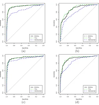
In addition we calculated the ROC curves for each of the three metrics. In order to do this we performed a 1-fold cross validation. That is, we removed an observation and then using
the parameters α and k which are given in Table 1 (since they produced the best results)
we classified it. This procedure was repeated for all observations. Thus, we ended up with the predicted membership values for all observations based on the 3 metrics. This allowed us to draw the ROC curves for each tributary when all 3 metrics were used. The results are presented in Figure 7.
We can see that for all tributaries the ROC curves of the ES-OVαmetric (3) and the TCα
lowest.
Specificity
Sensitivity
0.0
0.2
0.4
0.6
0.8
1.0
1.0 0.8 0.6 0.4 0.2 0.0
ESOVα
TCα
Aitchisonian
Specificity
Sensitivity
0.0
0.2
0.4
0.6
0.8
1.0
1.0 0.8 0.6 0.4 0.2 0.0
ESOVα
TCα
Aitchisonian
(a) (b)
Specificity
Sensitivity
0.0
0.2
0.4
0.6
0.8
1.0
1.0 0.8 0.6 0.4 0.2 0.0
ESOVα
TCα
Aitchisonian
Specificity
Sensitivity
0.0
0.2
0.4
0.6
0.8
1.0
1.0 0.8 0.6 0.4 0.2 0.0
ESOVα
TCα
Aitchisonian
[image:11.595.134.456.91.432.2](c) (d)
Figure 7: ROC curves for all tributaries using the three metrics For ES-OVαwe usedα = 0.35
and k= 2 and for TCα we used α = 0.5 andk = 2. For Each plot corresponds to one of the
four tributaries (a) Anoia, (b) Cardener, (c) Upper Llobregat and (d) Upper Llobregat.
Example 2. Forensic glass data with zero values
In the second example we will use the forensic glass dataset which has 214 observations from 6 different categories of glass with 8 chemical elements, in percentage form. The categories which occur are containers (13 observations), vehicle headlamps (29 observations), tableware (9 observations), vehicle window glass (17 observations), window float glass (70 observations) and window non-float glass (76 observations). This dataset contains a large number of zeros as well, thus excluding LRA from being applied here. The data are available from the UC Irvine Machine Learning Repository.
An interesting feature of this dataset is that it contains many zero values. This means
that the Aitchisonian metric (6) is not to be used. The ES-OVα and the TCα metrics on
the other hand are not affected by the presence of zeros, since 0 log 0 = 0. In this example the sample size of the test data was equal to 30, hence we used 184 compositional vectors to
train thek-NN algorithm. Again, the test data were chosen via stratified random sampling
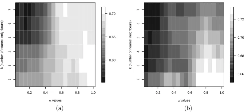
to avoid having categories not been selected in the test sample. Figure 8 shows the estimated
0.2 0.4 0.6 0.8 1.0
2
3
4
5
6
7
α values
k (n
umber of nearest neighbours) 0.60
0.65 0.70
0.2 0.4 0.6 0.8 1.0
2
3
4
5
6
7
α values
k (n
umber of nearest neighbours)
0.66 0.68 0.70 0.72
[image:12.595.95.497.85.269.2](a) (b)
Figure 8: The estimated percentage of correct classification for the forensic glass data as a
function ofk, the nearest neighbours and of α using the (a) ES-OVα metric (3) and (b) TCα
(5).
This is a simpler case to draw conclusions, since the best results are obtained whenα= 1
andk = 2 for both metrics, thus the ES-OV (2) and the TC (4) metrics should be used, with
the estimated percentage of correct classification being 71.45% and 73.35% respectively. Table
2 presents analytical information of the classification results. Estimates of the sensitivities and of the specificities for each category of glass are also given.
The mean sensitivities of ES-OVα metric (3) for Tableware and Vehicle window are low
and the same is true for the Vehicle window when TCα (5) is used. We observed that
many times, Tableware and Vehicle window were being wrongly classified as Vehicle float. A possible reason for this could be the small sample size of Tableware (this type of glass had the minimum number of observations). A chemist or a forensic scientist could perhaps give a possible answer to this (if that is the case of these types of glass being of similar structure). The ROC curves for each glass category (based on 1-fold cross validation) using both metrics are presented in Figure 9. We cannot say that one metric does better than the other always. For some glass categories, the two ROC curves are similar and for some others one seems a bit better than the other.
4
Conclusions
We suggested the use of a recently developed metric (2), for supervised classification when
the k-NN algorithm is implemented. We also added a free parameter to the metric with the
intention of improving the classification results. This free parameter was used to generalize
the taxicab metric as well. The examples showed that both the ES-OVα (3) and the taxicabα
(5) metric can be used for supervised clustering of compositional data, but can also be used in other scenarios as well.
ES-OVα
Tuning parameters Percentage of Glass Sensitivities Specificities
correct classification categories
α= 1 & k=3 71.45% (7.76%) Containers 77.25%(29.57%) 97.46%(2.76%)
Vehicle headlamps 80.88%(16.99%) 96.44%(3.60%)
Tableware 36.50%(48.26%) 96.95%(3.00%)
Vehicle window 29.25%(31.81%) 97.50%(2.97%)
Vehicle float 81.65%(11.60%) 82.30%(7.28%)
Non-window float 68.55%(13.39%) 90.50%(6.30%)
TCα
Tuning parameters Percentage of Glass Sensitivities Specificities
correct classification categories
α= 1 & k=3 73.35% (8.00%) Containers 77.75%(30.37%) 98.18%(2.43%)
Vehicle headlamps 82.62%(16.66%) 99.15%(1.77%)
Tableware 74.50%(43.70%) 98.14%(2.70%)
Vehicle window 29.75%(31.74%) 95.48%(3.71%)
Vehicle float 77.90%(12.58%) 82.10%(7.52%)
Non-window float 72.86%(14.45%) 90.11%(6.99%)
Table 2: Classification results for the forensic glass data. The number inside the parentheses indicates the standard error of the percentages.
naturally. This implies that no zero value replacement is necessary either parametrically (Martin et al., 2012) or non parametrically (Aitchison, 2003). In order to appreciate the importance of this advantage one can think of large datasets with many zeros.
The two metrics outbalanced the Aitchisonian metric (6) in the examples presented in
this manuscript. When it comes to comparing the the ES-OVα (3) and the taxicabα (5)
metric between them we cannot say one is better than the other.
A closer examination of the ROC curves revealed valuable information, especially for the FGL data example (where zeros are present) regarding the classification abilities of the
ES-OVα (3) and the taxicabα (5) metric. The sensitivities and specificities revealed interesting
patterns of the misclassification rates not captured by the percentage of correct classification. In addition, the ROC curves provided graphical evidence as for the ability of each metric to classify the observations.
Acknowledgements
Specificity
Sensitivity
0.0
0.2
0.4
0.6
0.8
1.0
1.0 0.8 0.6 0.4 0.2 0.0 ESOVα TCα
Specificity
Sensitivity
0.0
0.2
0.4
0.6
0.8
1.0
1.0 0.8 0.6 0.4 0.2 0.0 ESOVα TCα
Specificity
Sensitivity
0.0
0.2
0.4
0.6
0.8
1.0
1.0 0.8 0.6 0.4 0.2 0.0 ESOVα TCα
(a) (b) (c)
Specificity
Sensitivity
0.0
0.2
0.4
0.6
0.8
1.0
1.0 0.8 0.6 0.4 0.2 0.0 ESOVα TCα
Specificity
Sensitivity
0.0
0.2
0.4
0.6
0.8
1.0
1.0 0.8 0.6 0.4 0.2 0.0 ESOVα TCα
Specificity
Sensitivity
0.0
0.2
0.4
0.6
0.8
1.0
1.0 0.8 0.6 0.4 0.2 0.0 ESOVα TCα
[image:14.595.75.517.71.372.2](d) (e) (f)
Figure 9: ROC curves for all tributaries using the three metrics In all cases α = 1 and
k= 3 were used in both metrics. Each plot corresponds to one of the six glass categories (a)
containers, (b) vehicle headlamps, (c) tableware, (d) vehicle window glass, (e) window float glass and (f) window non-float glass.
References
Aitchison, J. (1982). The statistical analysis of compositional data. Journal of the Royal
Statistical Society. Series B, 44(2): 139–177.
Aitchison, J. (1992). On criteria for measures of compositional difference. Mathematical
Geology, 24(4): 365–379.
Aitchison, J. (2003). The Statistical Analysis of Compositional Data (Reprinted with addi-tional material by The Blackburn Press). London (UK): Chapman & Hall.
Baxter, M. J., Beardah, C. C., Cool, H. E. M., and Jackson, C. M. (2005). Compositional
data analysis of some alkaline glasses. Mathematical Geology, 37(2): 183–196.
Endres, D. M. and Schindelin, J. E. (2003). A new metric for probability distributions.
Information Theory, IEEE Transactions on, 49(7): 1858–1860.
Fry, J. M., Fry, T. R. L., and McLaren, K. R. (2000). Compositional data analysis and zeros
in micro data. Applied Economics, 32(8): 953–959.
Gallo, M. (2010). Discriminant partial least squares analysis on compositional data.Statistical
Mart´ın-Fern´andez J.A., Hron, K., Templ M., Filzmoser P. and Palarea-Albaladejo, J. (2012). Model-based replacement of rounded zeros in compositional data: Classical and robust
approaches. Computational Statistics & Data Analysis 56(9): 2688–2704.
Miller, W.E. (2002). Revisiting the geometry of a ternary diagram with the half-taxi metric.
Mathematical geology, 34(3): 275–290.
Neocleous, T., Aitken, C., and Zadora, G. (2011). Transformations for compositional data
with zeros with an application to forensic evidence evaluation. Chemometrics and
Intelli-gent Laboratory Systems, 109(1): 77–85.
Osterreicher, F. and Vajda, I. (2003). A new class of metric divergences on probability spaces
and its applicability in statistics. Annals of the Institute of Statistical Mathematics, 55(3):
639–653.
Otero, N., Tolosana-Delgado, R., Soler, A., Pawlowsky-Glahn, V., and Canals, A. (2005). Relative vs. absolute statistical analysis of compositions: A comparative study of surface
waters of a mediterranean river. Water Research, 39(7) 1404–1414.
Owen A.B. (2001). Empirical likelihood. Boca Raton: CRC Press.
Rodrigues, P. C. and Lima, A. T. (2009). Analysis of an European union election using
principal component analysis. Statistical Papers, 50(4): 895–904.
Scealy, J. L. and Welsh, A. H. (2011a). Properties of a square root transformation regression
model. In Proceedings of the 4th Compositional Data Analysis Workshop, Girona, Spain.
Scealy, J. L. and Welsh, A. H. (2011b). Regression for compositional data by using
distribu-tions defined on the hypersphere. Journal of the Royal Statistical Society. Series B, 73(3):
351–375.
Scealy, J. L. and Welsh, A. H. (2014). Fitting kent models to compositional data with small
concentration. Statistics and Computing, 24(2): 165–179.
Stephens, M. A. (1982). Use of the von Mises distribution to analyse continuous proportions.
Biometrika, 69(1): 197–203.
Stewart, C. and Field, C. (2011). Managing the essential zeros in quantitative fatty acid
signature analysis.Journal of Agricultural, Biological, and Environmental Statistics, 16(1):