A more general theory of commodity bundling

Munich Personal RePEc Archive

A more general theory of commodity

bundling

Armstrong, Mark

Department of Economics, University of Oxford

March 2012

Online at

https://mpra.ub.uni-muenchen.de/37375/

A More General Theory of Commodity Bundling

Mark Armstrong

University of Oxford

March 2012

Abstract

This paper extends the standard model of bundling as a price discrimination device to allow products to be substitutes and for products to be supplied by sep-arate sellers. Whether integrated or sepsep-arate, …rms have an incentive to introduce a bundling discount when demand for the bundle is elastic relative to demand for stand-alone products. Product substitutability typically gives an integrated …rm a greater incentive to o¤er a bundle discount (relative to the model with additive pref-erences), while substitutability is often the sole reason why separate sellers wish to o¤er inter-…rm discounts. When separate sellers coordinate on an inter-…rm discount, they can use the discount to overturn product substitutability and relax competition.

1

Introduction

Bundling—the practice whereby consumers are o¤ered a discount if they buy several

dis-tinct products—is used widely by …rms, and is the focus of a rich economic literature.

However, most of the existing literature discusses the phenomenon under relatively re-strictive assumptions, namely a consumer’s valuation for a bundle of several products is

the sum of her valuations for consuming the items in isolation, and bundle discounts are

only o¤ered for products sold by the same …rm. The two assumptions are related, in that

when valuations are additive it is less likely that a …rm would wish to reduce its price to a

customer who also buys a product from another seller. This paper analyzes the incentive

to engage in bundling when these assumptions are relaxed.

There are very many situations in which modelling products as substitutes is relevant.

For instance, when visiting a city a tourist may gain some extra utility from visiting art

gallery Aif she has already visited art galleryB, but the incremental utility is likely to be

smaller than if she were only to visitA. Joint purchase discounts (or premia) on products

o¤ered by separate sellers are rarer, though some examples include:

— A tourist may be able to buy a “city pass”, so that she can visit all participating tourist

attractions at a discount on the sum of individual entry fees. These could be organized

either as a joint venture by the attractions themselves, or implemented by an intermediary

which puts together its own bundles given wholesale fees negotiated with attractions.

— Bundling is prevalent in markets for transport services, as is the case with alliances between airlines or when neighboring ski-lifts o¤er a combined ticket.

— Products supplied by separately-owned …rms are often marketed together with discounts

for joint purchase. Thus, supermarkets and gasoline stations may cooperate to o¤er a

discount when both services are consumed. Airlines and car rental …rms may link up

for marketing purposes, and sometimes credit cards o¤er discounts proportional to spend

towards designated ‡ights or hotels.

— Pharmaceuticals are sometimes used as part of a “cocktail” with one or more drugs

supplied by other …rms. Drugs companies can set di¤erent prices depending on whether

the drug is used on a stand-alone basis or in a cocktail.

— Marketing data may reveal useful information about a potential customer’s purchase

history which a¤ects a …rm’s price to the customer. For instance, information that the

customer has chosen to buy …rm 1’s product may induce …rm 2 to discount its price, and

an inter-…rm discount for the joint purchase of the two products is implemented.

— At a wholesale level, a manufacturer may o¤er a retailer a discount if the retailer does

not stock a rival manufacturer’s product. (Such contracts are sometimes termed “loyalty

contracts”.) This is a situation with a bundle premium instead of a discount.

The plan of the paper is as follows. In section 2, I present a general framework for

consumer demand for two products in the presence of product substitutability and bundle discounts. Section 3 covers the case where an integrated …rm supplies both products.

I revisit the approach to bundling presented in Long (1984), which is used as a major

ingredient for the analysis in section 3. Long’s result is that the …rm has an incentive to

bundle when demand for the bundle is more elastic than demand for stand-alone products.

Relative to the situation with additive preferences, the integrated …rm typically has a

greater incentive to o¤er a bundle discount when products are substitutable. Because

the purchase of one product can decrease a consumer’s incremental utility from a second,

the …rm has a direct incentive to reduce the price for a second item, in addition to the

additive preferences.

In section 4 I turn to the situation where products are supplied by separate sellers.

With additive preferences, a …rm has a unilateral incentive to o¤er a bundle discount when

product valuations are negatively correlated. When there is full market coverage, a …rm

has an incentive to o¤er a joint-purchase discount under plausible conditions on consumer

valuations. When products are substitutes, whether a …rm has a unilateral incentive to

introduce a discount depends on the way that preferences are modelled. When there is a constant disutility of joint consumption, separate sellers typically wish to o¤er a

joint-purchase discount: the fact that a customer has joint-purchased the rival product implies that

her incremental valuation for the …rm’s own item has fallen, and this usually implies that

the …rm would like to reduce its price to this customer. Alternatively, if a proportion

of buyers only want a single item (for instance, a tourist in a city might only have time

to visit a single museum) while other consumers have additive preferences, a seller would

like, if feasible, to charge a premium when a customer also buys the rival product. In

examples, when this form of price discrimination is feasible, one price increases and the

other decreases relative to the situation with uniform pricing, and price discrimination results in higher equilibrium pro…t and higher welfare, but a worse outcome for consumers.

Finally, section 5 investigates partial coordination between separate sellers, which is

currently the relevant case for several of the industries mentioned above. Speci…cally, I

suppose that …rms …rst agree on a bundle discount which they fund jointly, and

subse-quently choose prices without coordination. When valuations are additive, it is shown that

such a scheme will usually raise each …rm’s pro…t, and, at least in the example considered,

its operation will also boost total welfare. However, when sellers o¤er substitute products,

the negotiated discount overturns the innate substitutability of products, inducing …rms to

raise prices. The resulting “tari¤-mediated” product complementarity can induce collusion which harms consumers and overall welfare.

This paper is not the …rst to investigate these issues. The incentive for an integrated

seller to o¤er a discount for the purchase of multiple items is discussed by Adams and Yellen

(1976), Long (1984) and McAfee, McMillan, and Whinston (1989), among many others.

The latter two papers showed that it is optimal to introduce a bundle discount whenever the

distribution of valuations is statistically independent and valuations are additive, so that a

degree of joint pricing is optimal even with entirely unrelated products. Except for Long,

these papers assume that valuations are additive.1 _{Long (1984) presents what could be}

termed an “economic” model of bundling. Rather than following a diagrammatic exposition

concentrating on the details of joint distributions of two-dimensional consumer valuations,

he uses standard demand theory—which applies equally to non-additive preferences—to

derive conditions under which a bundle discount is optimal.

Schmalensee (1982) and Lewbel (1985) study the incentive for a single-product

monop-olist to o¤er a discount if its customers also purchase a competitively-supplied product.

Schmalensee supposes that two items are for sale to a population of consumers, and item 1 is available at marginal cost due to competitive pressure while item 2 is supplied by a

monopolist. Valuations are additive, but are not independent in the statistical sense. If

there is negative correlation in the values for the two items, the fact that a consumer buys

item 1 is “bad news” for the monopolist, who then has an incentive to set a lower price to

its customers who also buy 1. Lewbel performs a similar exercise but allows the two items

to be partial substitutes. In this case, the fact that a consumer buys item 1 is also bad

news for the monopolist, and gives an incentive to o¤er a discount for joint consumption.

Bundling arrangements between separate …rms are analyzed by Gans and King (2006),

who investigate a model with two kinds of products (gasoline and food, say), and each product is supplied by two di¤erentiated …rms. When all four products are supplied by

separate …rms which set their prices independently, there is no interaction between the two

kinds of product. However, two …rms (one o¤ering each of the two kinds of product) can

enter into an alliance and agree to o¤er consumers a discount if they buy both products from

the alliance. (In their model, the joint pricing mechanism is similar to that used in section

5 below: …rms decide on their bundle discount, which they agree to fund equally, and

then set prices non-cooperatively.) Gans and King observe that when a bundle discount is

o¤ered for joint purchase of otherwise independent products, those products are converted

into complements. In their model, in which consumer tastes are uniformly distributed, a pair of …rms does have an incentive to enter into such an alliance, but when both pairs

do this their equilibrium pro…ts are unchanged from the situation when all four …rms set

independent prices, although welfare and consumer surplus fall.2

Calzolari and Denicolo (2011) propose a model where consumers buy two products

and each product is supplied by a single …rm. Each …rm potentially o¤ers a nonlinear

example, and a consumer’s valuation for the bundle is some constant proportion (greater or less than one, depending on whether complements or substitutes are present) of the sum of her stand-alone valuations. The focus of their analysis is on whether pure bundling is superior to linear pricing.

tari¤ which depends on a buyer’s consumption of its own product and her consumption

of the other …rm’s product. They …nd that the use of these tari¤s can harm consumers

compared to the situation in which …rms base their tari¤ only on their own supply. Their

model di¤ers in two ways from the one presented in section 4 of this paper. First, in

their model consumers have elastic (linear) demands, rather than unit demands, for the

two products. Thus, they must consider general nonlinear tari¤s, while the …rms in my

model merely choose a pair of prices. Second, in my model consumers di¤er in richer way, and a consumer might like product 1 but not product 2, and can vary in the degree of

substitutability between products. In Calzolari and Denicolo (2011), consumers di¤er by

only a scalar parameter (the demand intercept for both products), and so all consumers

view the two products when consumed alone as perfect substitutes.

Finally, Lucarelli, Nicholson, and Song (2010) discuss the case of pharmaceutical

cock-tails. Although the focus of their analysis is on situations in which …rms set the same

price for a drug, regardless of whether it is used in isolation or as part of a cocktail, they

also consider situations where …rms can set two di¤erent prices for the two kinds of uses.

They document how a …rm selling treatments for HIV/AIDS set di¤erent prices for similar chemicals depending on whether the drug was part of a cocktail or not. They estimate a

demand system for colorectal cancer drugs, where there are at least 12 major drug

treat-ments, 6 of which were cocktails combining drugs from di¤erent …rms. Although in this

particular market …rms do not price drugs di¤erently depending whether the drug is used

in a cocktail, they estimate the impact when one …rm engages in this form of price

dis-crimination. They …nd that a …rm will typically (but not always) reduce the price for

stand-alone use and raise the price for bundled use.

2

A Framework for Consumer Demand

Consider a market with two products, labeled 1 and 2, where a consumer buys either

zero or one unit of each product (and maybe one unit of each). A consumer is willing to

pay vi for product i = 1;2 on its own, and to pay vb for the bundle of both products. (A consumer obtains payo¤ zero if she consumers neither product.) Thus a consumer’s

preferences are described by the vector (v1; v2; v_b), which varies across the population of

consumers according to some known distribution.3 _{A consumer views the two products}

3_{In the analysis which follows, we assume that the stand-alone valuations (v}

1; v2) have a continuous

marginal density with support on a compact rectangle in R2

+. Given (v1; v2), the distribution of vb is

as partial substitutes whenever vb v1 + v2. Whenever there is free disposal, so that

a consumer can discard an item without cost, we require that vb maxfv1; v2g for all

consumers.

Only deterministic selling procedures are considered in this paper.4 _{Consumers face}

three prices: p1 is the price for consuming product 1 on its own;p2 is the price for product

2 on its own, and p1 +p2 is the price for consuming the bundle of both products.

Thus, is the discount for buying both products, which is zero if there is linear pricing or negative if consumers are charged a premium for joint consumption. A consumer chooses

the option from the four discrete choices which leaves her with the highest surplus, so she

will buy both items whenever vb (p1+p2 ) maxfv1 p1; v2 p2;0g, she will buy

product i = 1;2 on its own whenever vi pi maxfvb (p1+p2 ); v_j p_j;0g, and

otherwise she buys nothing.

As functions of the three tari¤ parameters (p1; p2; ), denote by Q1 the proportion of

potential consumers who buy only product 1, Q2 the proportion who buy only product 2,

and Qb the proportion who choose the bundle. It will also be useful to discuss demand when no discount is o¤ered, so let qi(p1; p2) Q_i(p1; p2;0) and q_b(p1; p2) Q_b(p1; p2;0)

be the corresponding demand functions when = 0. Indeed, we will see that a …rm’s incentive to introduce a bundle discount is determined entirely by the properties of the

“no-discount” demandsqi and qb. This is important insofar as these demand functions are easier to estimate from market data than the more hypothetical demands Qi and Qb.5

Several properties of these demand functions follow immediately from the discrete

choice nature of the consumer’s problem, and are not contingent on whether the

prod-ucts are partial substitutes. To illustrate, note that total demand for each product is an

increasing function of the bundle discount, i.e.,

Qi+Qb increases with . (1) su¢ciently well behaved that the demand functions shortly de…ned are di¤erentiable.

4_{Unlike the single-product case, when a monopolist sells two or more products it can often increase its} pro…ts if it is able to use stochastic schemes (e.g., where for a speci…ed price the consumer gets product 1 or product 2 but she is not sure which one). See Pavlov (2011) for a recent contribution to this topic, which studies cases with extreme substitutes (all consumers buy a single item) and with additive preferences.

To see this, observe that a consumer buys product 1, say, if and only if

maxfvb (p1 +p2 ); v1 p1g maxfv2 p2;0g :

(The left-hand side above is the consumer’s maximum surplus if she buys product 1—either

in the bundle or on its own—while the right-hand side is the consumer’s maximum surplus

if she does not buy the product.) Clearly, the set of such consumers is increasing (in the

set-theoretic sense) in . In the case of separate supply, analyzed in section 4, this implies that when a …rm unilaterally introduces a bundle discount, its rival’s pro…ts will rise.

We necessarily have Slutsky symmetry of cross-price e¤ects, so that

@Q2

@p1

+@Q2

@

@Q1

@p2

+@Q1

@ ;

@Qb

@pi

+@Qb

@

@Qi

@ : (2)

For instance, the left-hand side of (2) says that the e¤ect on demand for good 2 on its own

of a price rise of good 1 on its own (which is achieved by increasingp1 and by the same

amount so that the bundle price does not change) is the same as the e¤ect on demand

for good 1 on its own of price rise for good 2 on its own. Setting = 0 in the right-hand expression in (2) implies that the impact of a small bundle discount on the total demand for a product is equal to the impact of a corresponding price cut on bundle demand, i.e.,

@(Qi+Qb)

@ =0

= @qb

@pi

: (3)

This identity plays a key role when we analyze the pro…tability of introducing a discount.

One price e¤ect which does depend on the innate substitutability of products is the

following:

Claim 1 Suppose that vb v1+v2 for all consumers. Then when linear prices are used,

demand for product i,qi+qb, weakly increases with pj.

(All omitted proofs are contained in the appendix.) Importantly, when a bundle discount

is o¤ered, this result can be reversed: even if products are intrinsically substitutes then

when >0 the demand for a product can decrease with the stand-alone price of the other product. The observation that a bundle discount can overturn the innate substitutability

of products is a recurring theme in the following analysis.

A second property of demand which depends on product substitutability is that any consumer who chooses to buy the bundle at linear prices (p1; p2) has v_j p_j for each

j = 1;2. To see this, note that if a consumer with preferences (v1; v2; v_b)buys the bundle

follows from substitutability and the second is due to the superiority of the bundle to

production its own. Thus,minfv1 p1; v2 p2g 0. This implies that with linear pricing

there is no “margin” between buying the bundle and buying nothing, and any consumer

who optimally buys the bundle would instead buy a single item (if they change at all) rather

than exit altogether when faced with a small price rise. A second implication is that the set

of consumers who buysomethingwith linear prices(p1; p2)consists of those consumers with

preferences satisfyingmaxfv1 p1; v2 p2g 0. (Clearly, ifv_i p_i then the consumer will

buy something, since product i on its own yields positive surplus. Those consumers who

buy the bundle lie inside this set since they satisfyminfv1 p1; v2 p2g 0.) In particular,

the fraction of participating consumers, which isq1(p1; p2)+ q2(p1; p2) +q_b(p1; p2), depends

only on the (marginal) distribution of the stand-alone valuations (v1; v2).

3

Integrated Supply

3.1

Long’s analysis revisited

Suppose that the market structure is such that an integrated monopolist supplies both

products. Here, and in section 4 with separate supply, suppose that the constant marginal

cost of supplying productiis equal toci. To avoid tedious caveats involving corner solutions in the following analysis, suppose that over the relevant range of linear prices there is some

two-item demand, so that qb >0.

In this section I recapitulate the analysis in Long (1984), as the integrated-…rm analysis throughout section 3 rests on this. The …rm’s pro…t with bundling tari¤ (p1; p2; )is

= (p1 c1)(Q1+Q_b) + (p2 c2)(Q2 +Q_b) Q_b : (4)

Consider the incentive to o¤er a bundle discount. Starting from linear prices (p1; p2), by

di¤erentiating (4) we see that the impact on pro…t of introducing a small discount >0is

@

@ =0

= (p1 c1)

@

@ (Q1+Qb) + (p2 c2) @

@ (Q2+Qb) Qb =0 = (p1 c1)

@qb

@p1

(p2 c2)

@qb

@p2

qb ; (5)

where the second equality follows from expression (3).

Although Long also considers the asymmetric case, his analysis is greatly simpli…ed

when products are symmetric, and for the remainder of section 3 assume thatc1 =c2 =c

and the same density of consumers have taste vector(v1; v2; v_b)as have the permuted taste

tari¤s which are symmetric in the two products. If the …rm o¤ers pricepfor either product

and no bundle discount, writexs(p)andxb(p)respectively for the proportion of consumers who buy a single item and who buy the bundle. (Thus, xs(p) q1(p; p) +q2(p; p) and

xb(p) qb(p; p).) From expression (5), a small discount is pro…table with stand-alone price

p in this symmetric setting if and only if

xb(p) + (p c)x0b(p)<0: (6)

Consider whether this is satis…ed at the most pro…table linear price,p . Sincep maximizes

(p c)(xs(p) + 2xb(p)), the …rst-order condition for p is

xs(p ) + 2xb(p ) + (p c)(x0s(p ) + 2x

0

b(p )) = 0 :

Taking this together with expression (6), we see that it is pro…table to introduce a bundle

discount if

x0

b(p )

xb(p )

> x

0

s(p )

xs(p )

so that bundle demandxb is more elastic than single-item demand xs at optimal price p . This discussion is summarized in this result:6

Proposition 1 Suppose an integrated monopolist supplies two symmetric products. The

…rm has an incentive to introduce a discount for buying the bundle whenever the demand

for a single item is less elastic than the demand for the bundle, so that

xb(p)

xs(p)

strictly decreases with p : (7)

Condition (7) is intuitive: if the …rm initially charges the same price for buying a single

item as for buying a second item, and if demand for the latter is more elastic than demand

for the former, then the …rm would like to reduce its price for buying a second item (and

to increase its price for the …rst item).

Consider the familiar knife-edge case where a consumer’s valuation for the bundle is

the sum of her stand-alone valuations, i.e., vb v1+v2. With additive valuations, if the

…rm o¤ers the linear price pfor buying either item the consumer’s decision is simple: she

should buy product i whenever vi p. De…ne

(p) Prfv2 pjv1 pg ; (8)

6_{Long stated the result in the alternative, but equivalent, form whereby bundling was pro…table if the} ratio of total demandxs+ 2xb to the number of customers xs+xb decreased when the pricepincreased.

When products are not symmetric, Long shows using a similar analysis that the …rm has an incentive to introduce a discount for buying the bundle whenever single-item demand is less elastic than bundle demand, in the sense that qb=(q1+q2)strictly decreases with an equi-proportional ampli…cation of

so that

(p) = xb(p)

xb(p) +

1 2xs(p)

and

xb(p)

xs(p)

= 1 2

(p) 1 (p) :

Proposition 1 implies, therefore, that the …rm has an incentive to introduce a bundle

discount if

(p) strictly decreases withp (9) (at the most pro…table linear price p ). Condition (9) holds, roughly speaking, if v1 and v2

are not “too” positively correlated. In particular, a degree of bundling is pro…table even

if valuations are additive and statistically independent. As we explore in the next section,

the more fundamental condition (7) is also useful for situations outside this additive case.

3.2

Bundling with substitute products

Using Long’s condition (7), in this section I analyze in more detail the …rm’s incentive to

bundle when preferences are not additive. One advantage of assuming symmetry in the

two products is that what is in general the three-dimensional nature of preferences reduces

to just two dimensions, since only the highest stand-alone valuation matters out of(v1; v2).

With this in mind, given preferences (v1; v2; v_b), de…ne

V1 maxfv1; v2g ; V2 v_b V1 ; (10)

so that V1 is a consumer’s maximum utility if she buys only one item and V2 is her

incre-mental utility from the second item. Note thatvb =V1+V2, so that valuations are additive

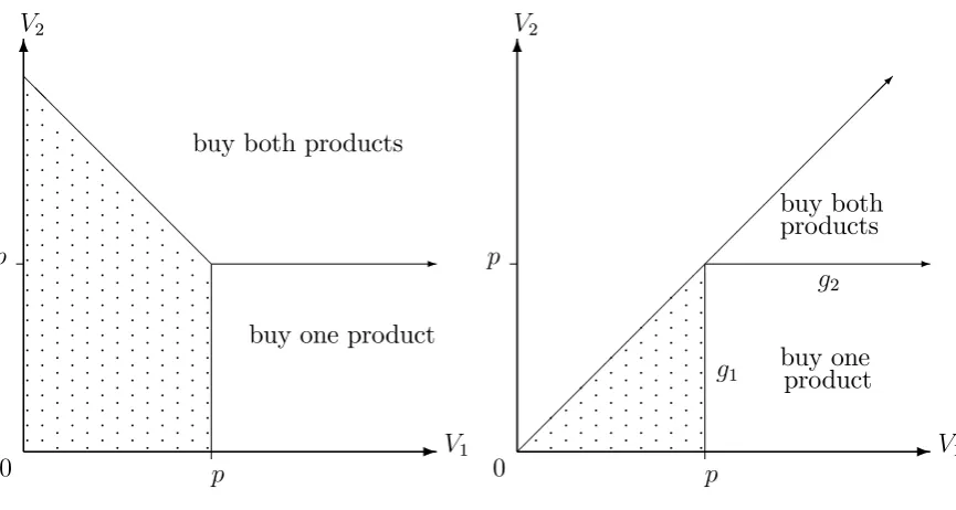
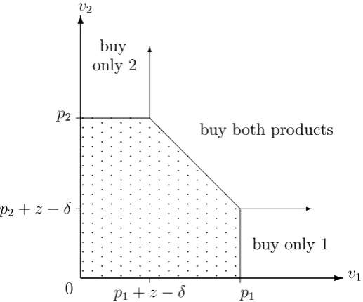
after this change of variables. Given the linear pricepfor each item, the type-(V1; V2)

con-sumer will buy one item if V1 p and V2 < p, and she will buy both items if V2 p and

V1+V2 2p, and this pattern of demand is depicted on Figure 1A. In general, a consumer

might buy both items even if she does not obtain positive surplus from buying only one, so

there is a “margin” between buying the bundle and buying nothing. However, if products

are substitutes this margin disappears: whenvb v1+v2 thenV2 minfv1; v2g V1, and

the support of (V1; V2)lies under the 45 0

line as shown on Figure 1B.

From now on, assume that the products are substitutes. Similarly to (8), de…ne

(p) PrfV2 pjV1 pg=

PrfV2 pg PrfV1 pg

: (11)

By examining Figure 1B we see that xb = (xb+xs) , or

xb(p)

xs(p)

-6 -@ @ @ @ @ @ @ @ @ 0 _p p V1 V2

buy one product buy both products

p p p p p p p p p p p p p p p p p p p p p p p p p p p p p p p p p p p p p p p p p p p p p p p p p p p p p p p p p p p p p p p p p p p p p p p p p p p p p p p p p p p p p p p p p p p p p p p p p p p p p p p p p p p p p p p p p p p p p p p p p p p p p p p p p p p p p p p p p p p p p p p p p p p p p p p p p p p p p p p p p p p p p p p p p p p p p p p p p p p p p p p p p p p p p p p p p p p p p p p p p p p p p p p p p p p p p p p p p p p p p p p p p p p p p p p p p p -6 -g1 g2 0 _p p V1 V2 buy one product buy both products

p _pp p p p p p p p p p p p p p p p p p p p p p p p p p p p p p p p p p p p p p p p p p p p p p p p p p p p p p p p p p p p p p p p p p p p p p p p p p p p p p p p p

Figure 1A: General case Figure 1B: Substitute products

Therefore, when is strictly decreasing Proposition 1 implies that the monopolist has

an incentive to introduce at least a small bundle discount. In fact, we can obtain the

following non-local result, which is our main result for integrated supply:

Proposition 2 Suppose products are substitutes and in (11) is strictly decreasing. Then

the most pro…table bundling tari¤ for a monopolist involves a positive bundle discount.

The fundamental condition which makes bundling pro…table for an integrated seller

is (7), and this condition applies regardless of whether products are substitutes or not.

However, the more transparent condition that in (11) be decreasing only applies when

products are substitutes. Otherwise, the pattern of demand looks like Figure 1A above,

and does not capture all the relevant demand information.

For i = 1;2, write Gi(p) = PrfVi pg for the marginal c.d.f. for valuation Vi and

gi(p) = G0i(p) for the corresponding marginal density. (The densities g1 and g2 are the

“measures” of the lines marked on Figure 1B.) The condition that is decreasing is

equivalent to the hazard rates satisfying g1=(1 G1)< g2=(1 G2). As is well known, a

su¢cient condition for this to hold is that the likelihood ratio

g1(p)

g2(p)

decreases withp : (12)

Whenever (12) holds, then, the …rm has an incentive to introduce a bundle discount.

Proposition 2 applies equally to an alternative framework where the monopolist supplies

Here, the parameterV1 represents a consumer’s value of one unit andV2 is her incremental

value for the second. Thus when consumers have diminishing marginal utility (V2 V1)

and in (11) is decreasing, the single-product …rm will o¤er a nonlinear tari¤ which

involves a quantity discount.7 _{(However, this alternative interpretation of the model is not}

natural in the separate sellers context of section 4, since we would have to assume that for

some reason a supplier could only sell a single unit of the product to a consumer.)

A natural question is whether products being substitutes makes it more likely that the integrated …rm wishes to introduce a bundle discount, relative to the same market but

with additive valuations. Consider a market where the stand-alone valuations, v1 and v2,

have a given (symmetric) distribution. We know from Proposition 1 that the …rm has

an incentive to o¤er a bundle discount whenever xb=xs is decreasing in the linear price

p, which is equivalent to the condition that xb=n decreases with p, where n xs +xb is the fraction of consumers who buy something from the …rm. Consider two scenarios: in

scenario (a), each consumer’s valuation for the bundle is additive, so that vb v1 +v2,

while in scenario (b) we have vb v1+v2. Write the fraction of consumers who buy both

items at linear price p in scenario (a) as xb(p) and the corresponding fraction in scenario (b) asx^b(p). As discussed in section 2, n is exactly the same function in the two scenarios. Thus, if x^b=xb (weakly) decreases with price, then whenever bundling is pro…table under scenario (a) it is sure to be pro…table under scenario (b) as well. It is plausible, though

not inevitable, that demandx^b is more elastic than demand xb. Since V2 minfv1; v2g, it

follows that x^b xb. Thus, for x^b to be more elastic we require that the slope x^0b not be “too much” smaller than x0

b.8

Intuitively, when products are substitutes there is an extra motive to o¤er a bundle

discount, relative to the additive case, which is to try to serve customers with a second

item even though the incremental utility of the second item is lowered by the purchase of the …rst item. Once a customer has purchased one item, this is bad news for her

willingness-to-pay for the other item, and this often gives the …rm a motive to reduce price for the

7_{See Maskin and Riley (1984) for an early contribution to the theory of quantity discounts, where—in} contrast to the current paper—consumers di¤er by only a scalar parameter.

8_{An example where the substitutability of products makes the …rm less likely to engage in bundling} is as follows. Suppose that vb = v1+v2 if minfv1; v2g k and vb = maxfv1; v2g otherwise, where k

is a positive constant. Thus, preferences are additive when both stand-alone valuations are high, while if one valuation does not meet the threshold k the incremental value for the second item is zero. With these preferences, whenever the linear price satis…esp < kthose consumers with minfv1; v2g kwill buy

second item. With additive preferences, the only motive in this model to use a bundle

discount is to extract information rents from consumers, and this motive vanishes if the

…rm knows consumer preferences. With sub-additive preferences, the …rm may wish to

o¤er a bundling tari¤ even when it knows the customer’s tastes. While with integrated

supply sub-additive preferences merely give one additional reason to bundle, with separate

sellers such preferences will often be thesole reason to o¤er a bundle discount, as discussed

in section 4.

3.3

Special cases

In this section I describe three special cases to illustrate this analysis of bundling incentives,

as well as some equilibrium bundling tari¤s.

Example 1: Constant disutility of joint consumption.

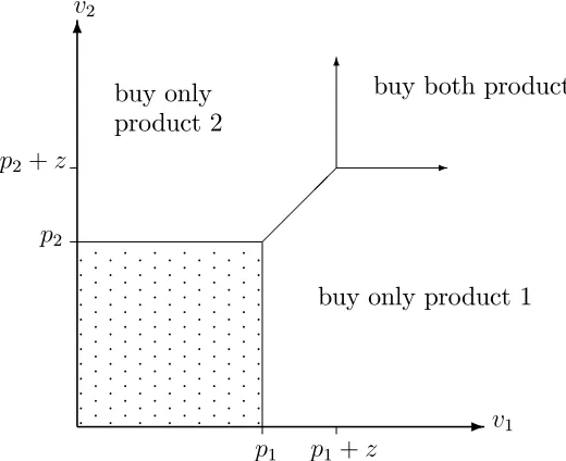
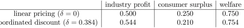
Consider the situation in which for all consumers

vb =v1+v2 z (13)

for some constant z 0. Here, to ensure free disposal we assume that the minimum possible realization of vi is greater thanz. With a linear price pi for buying product i, the pattern of demand is as shown on Figure 2. The next result provides a su¢cient condition

for bundling to be pro…table in this setting.

Claim 2 Suppose that bundle valuations are given by (13). Suppose that each valuation

vi has marginal c.d.f. F and marginal density f, and the hazard rate f( )=(1 F( )) is

strictly increasing. Then a monopolist has an incentive to o¤er a bundle discount when

condition (9) holds.

To illustrate, suppose that (v1; v2) is uniformly distributed on the unit square [1;2] 2

,

and that z = 1

4 and c = 1. Then an integrated monopolist which uses linear prices will

choosep 1:521, generating pro…t of around0:407. At this price, around 73% of potential consumers buy something, although only 5% buy both products. The most pro…table

bundling tari¤ can be calculated to be

p 1:594 ; 0:380 ; (14)

substitutability of the products (i.e., > z), and faced with this bundling tari¤ consumers

now view the two products as complements rather than substitutes. (The resulting pattern

of demand looks as depicted in Figure 5.) Nevertheless, the discount in (14) is smaller than

it is in the corresponding example with additive valuations (i.e., when z = 0).9

-6

-6

p1 p1+z

p2+z

p2

v1

v2

buy only product 1 buy both products buy only product 2 p p p p p p p p p p p p p p p p p p p p p p p p p p p p p p p p p p p p p p p p p p p p p p p p p p p p p p p p p p p p p p p p p p p p p p p p p p p p p p p p p p p p p p p p p p p p p p p p p p p p p p p p p p p p p p p p p p p p p p p p p p p p p p p p p p p p p p p p p p p p p p p p p p p p p p p p p p p p

Figure 2: Pattern of demand with constant disutility of joint purchase

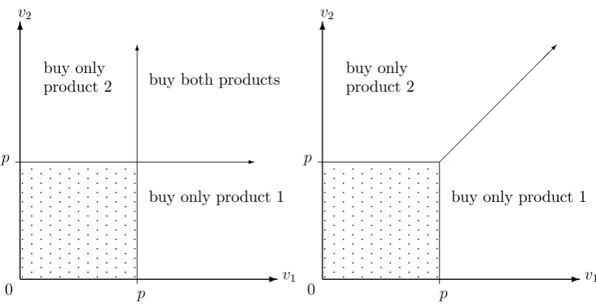
Example 2: Time-constrained consumers.

A natural reason why products might be substitutes is that some buyers are only

able to consume a restricted set of products, perhaps due to time constraints.10 _{To that}

end, suppose that an exogenous fraction of consumers have valuationvi for stand-alone product i= 1;2and valuation vb =v1+v2 for the bundle, while the remaining consumers

can only buy a single item (and have valuation vi if they buy item i). (See Figure 3 for an illustration.) For simplicity, suppose that the distribution for (v1; v2) is the same

for the two groups of consumers. Let ( ) be as de…ned in (8). It is straightforward to show (p) = (p)=(2 (p)), so that is decreasing if and only if is. Proposition 2 therefore implies that when some consumers are time-constrained, an integrated …rm

has an incentive to o¤er a bundle discount if and only if (9) holds, i.e., under the same

condition as when consumers have additive preferences. The reason is that when the …rm

o¤ers a bundle discount this only a¤ects the unconstrained consumers, and the sign of

the impact on pro…t is just as if all consumers had additive preferences.

9_{Whenc= 1, (v}

1; v2)is uniformly distributed on[1;2]2andvb v1+v2, one can check thatp=5₃ and

= p2

3 0:47:

-6 6 -0 _p p v1 v2

buy only product 1 buy both products buy only product 2 p p p p p p p p p p p p p p p p p p p p p p p p p p p p p p p p p p p p p p p p p p p p p p p p p p p p p p p p p p p p p p p p p p p p p p p p p p p p p p p p p p p p p p p p p p p p p p p p p p p p p p p p p p p p p p p p p p p p p p p p p p p p p p p p p p p p p p p p p p p p p p p p p p p p p p p p p p p p -6 0 _p p v1 v2

buy only product 1 buy only product 2 p p p p p p p p p p p p p p p p p p p p p p p p p p p p p p p p p p p p p p p p p p p p p p p p p p p p p p p p p p p p p p p p p p p p p p p p p p p p p p p p p p p p p p p p p p p p p p p p p p p p p p p p p p p p p p p p p p p p p p p p p p p p p p p p p p p p p p p p p p p p p p p p p p p p p p p p p p p p

Figure 3A: Unconstrained consumers Figure 3B: Time-constrained consumers

Example 3: Stand-alone values (v1; v2) are uniformly distributed on the unit square [0;1] 2

,

and given (v1; v2) the bundle value v_b is uniformly distributed on [maxfv1; v2g; v1+v2].

(Recall that with free disposal we require that vb be at least maxfv1; v2g, and we

require vb v1 +v2 if products are substitutes.) The support of (V1; V2) on Figure 1B

in this example is 0 V2 V1 1, and calculations reveal that the joint density for (V1; V2) on this support is 2 logV_V1

2. The marginal densities for V1 and V2 are respectively g1(p) = 2p and g2(p) = 2(p logp 1). It follows that x_b(p) = 1 (p

2

2plogp) and

xs(p) = 2plogp. If c= 0, the most pro…table linear pricepmaximizesp(xs(p) + 2xb(p)), which entailsp 0:540and pro…t 0.406. About 70% of potential consumers buy something with this tari¤, although just 4% of consumers buy the bundle.

One can check that xb=xs strictly decreases withp, and Proposition 1 implies that the …rm will wish to o¤er a bundle discount. One can modify Figure 1B to allow the …rm to

o¤er a discount >0, and integrate the density for(V1; V2)over the regions corresponding

to item and bundle demand, to obtain explicit (but tedious) expressions for

single-item and bundle demands in terms of the tari¤ parameters(p; ). Using these expressions, one can calculate the optimal bundling tari¤ to be p 0:648 and 0:588, which yields pro…t 0.463. Notice that the bundle discount is now deeper compared to the corresponding

example with additive values.11 _{With this bundling tari¤, where the incremental price for}

the second item is rather small, about 51% of potential consumers buy the bundle and

only 15% buy a single item.

11_{Whenc= 0, (v}

4

Separate Sellers

4.1

General analysis

I turn now to the situation where the two products are supplied by separate sellers. In

contrast to the integrated seller case, here there is no signi…cant advantage in assuming

that products are symmetric, and we no longer make that assumption. Suppose that the

sellers set their tari¤s simultaneously and non-cooperatively. (The next section discusses

a setting in which …rms coordinate on their inter-…rm bundle discount.) When …rms

o¤er linear prices—i.e., prices which are not contingent on whether the consumer also

purchases the other product—…rmi chooses its pricep_i given its rival’s price to maximize

(pi ci)(qi+qb), so that

qi 1 (pi ci)

@qi=@pi

qi

+qb 1 (pi ci)

@qb=@pi

qb

= 0 : (15)

In some circumstances, a …rm can condition its price on whether a consumer also buys

the other …rm’s product. For instance, a museum could ask a visitor to show her entry ticket

to the other museum to claim a discount. Suppose now that …rmi o¤ers a discount >0

from its price p_i to those consumers who purchase product j as well. (Those consumers who only buy product i continue to pay p_i.) Then …rmi’s pro…t is

i = (pi ci)(Qi+Qb) Qb ; (16) and the impact on pro…t of a small joint purchase discount is governed by the sign of

d i

d =0, which from (3) is equal to

qb (pi ci)

@qb

@pi

: (17)

When demand for the single item is less elastic than bundle demand, so that @qi=@pi

qi <

@qb=@pi

qb , the second term [ ]in (15) is strictly negative, i.e., (17) is strictly positive. In this

case, o¤ering a discount for joint purchase will raise the …rm’s pro…t.

Thus, discounts for joint purchase can arise even when products are supplied by

sep-arate …rms and when a …rm chooses and funds the discount unilaterally. The reason is

straightforward: since the own-price elasticity of bundle demand is higher than that of demand for its stand-alone product, a …rm wants to o¤er a lower price to those consumers

who also buy the other product. As expression (1) shows, the introduction of a discount

will also bene…t the rival …rm.

Proposition 3 Suppose that demand for the bundle is more elastic than demand for …rm

i’s stand-alone product, in the sense that

qb(p1; p2)

qi(p1; p2)

strictly decreases with pi : (18)

Starting from the situation where …rms set equilibrium linear prices p1 and p2, …rm i has

an incentive to o¤er a discount to those consumers who buy product j: If expression (18)

is reversed, so that qb=qi increases with pi, then …rm i would like if feasible to charge its

customers a premium if they buy product j.

The crucial di¤erence between condition (18) and the corresponding condition (7) with

integrated supply is that with a single seller both prices are increased, whereas with separate

sellers only one price rises. With substitute products and linear pricing, a …rm competes on three fronts. If it raises its price: (i) some consumers will switch from buying the

bundle to buying the rival product alone; (ii) some will switch from buying its product

alone to buying the rival product alone, and (iii) some consumers will switch from buying

its product alone to buying nothing. (As discussed in section 2, with substitutes a possible

fourth margin between buying the bundle and buying nothing is absent.) Broadly speaking,

condition (18) requires that margins (ii) and (iii) together are less signi…cant, relative to

the size of associated demand, than margin (i).

When products are asymmetric, at the equilibrium linear prices it is possible that one

…rm has an incentive to o¤er a discount when a customer also buys the other …rm’s product, but the other …rm does not.12 _{However, it may well be that both …rms choose to o¤er such}

a discount. If …rmi= 1;2o¤ers the pricepiwhen a consumer only buys its product and the price pi i when she also buys the other product, a consumer who buys the bundle pays the pricep1+p2 1 2. The issue then arises as to how the combined discount = 1+ 2

is implemented. For instance, a consumer might have to buy the two items sequentially,

and …rms cannot simultaneously require proof of purchase from the other seller when they

o¤er their discount. However, there are at least two natural ways to implement this

inter-…rm bundling scheme. First, the bundle discount could be implemented via an electronic

sales platform which allows consumers to buy products from several sellers simultaneously. Sellers choose their prices contingent on which other products (if any) a consumers buys,

a website displays the total prices for the various combinations, and …rms receive their

stipulated revenue from the chosen combination. With such a mechanism there is no need

for …rms to coordinate their tari¤s. Second, there may be “product aggregators” present

in the market who put together their own bundles from products sourced from separate

…rms and retail these bundles to …nal consumers. In the two-product case discussed in this

paper, aggregators bundle the two products together and each …rm chooses a wholesale

price for its product contingent on being part of the bundle. If the aggregator market is

competitive, the price of the bundle will simply be the sum of the two wholesale prices.

Again, there is no need for …rms to coordinate their prices.

A major di¤erence between this inter-…rm bundling discount and the discount o¤ered by

an integrated supplier is that with separate sellers the discount is chosen non-cooperatively.

A bundle is, by de…nition, made up of two “complementary” components, namely, …rm 1’s

product and …rm 2’s product, and the total price for the bundle is the sum of each …rm’s

component price pi i. When a …rm considers the size of its own discount i, it ignores the bene…t this discount confers on its rival. Thus, as usual with separate supply of

complementary components, double marginalization will result and the overall discount

= 1+ 2 will be too small (for given stand-alone prices).

4.2

Special cases

In this section, I analyze in more depth various special cases where separate sellers have

an incentive to introduce a joint-purchase discount. Consider …rst the situation where

consumer valuations are additive, so that margin (ii) discussed in section 4 is absent and

…rms do not compete with each other:

Proposition 4 Suppose that valuations are additive, i.e., vb = v1 +v2. Starting from

the situation where …rms set equilibrium linear prices, …rm i has an incentive to o¤er a

discount to those consumers who buy the other product whenever Prfvj p j vig strictly

increases with vi.

Whenever the valuations are negatively correlated in the strong sense that Prfvj pjvig decreases withvi, then, a …rm has an incentive to o¤er a discount for joint purchase. Some-what counter-intuitively, those …rms which o¤er products which appeal to very di¤erent

kinds of consumer (boxing and ballet, say) may wish to o¤er discounts to consumers who buy the other product.

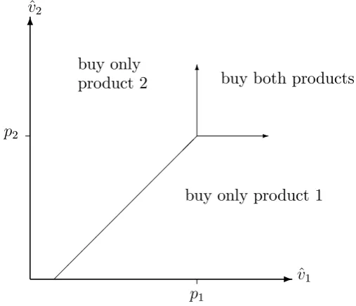
In the oligopoly context, it is sometimes natural to consider situations with full coverage,

so that all consumers buy something for the relevant range of linear prices.13 _{(This is}

relevant when the minimum possible realizations of v1 and v2 are su¢ciently high.) When

the outside option of zero is not relevant for any consumer’s choice, all that matters for

demand is the distribution of incremental utilities, and given the triple (v1; v2; v_b) de…ne

new variables

^

v1 v_b v2 ; ^v2 v_b v1 (19)

for the incremental valuation for producti given the consumer already has productj.

-6

-6

p1

p2

^

v1 ^

v2

buy only product 1 buy both products buy only

product 2

Figure 4: Pattern of demand with full consumer coverage

As depicted on Figure 4, a consumer will buy both items with linear prices (p1; p2)

provided that v^1 p1 and ^v2 p2, and otherwise she will buy product 1 instead of

product 2 when v^1 p1 v^2 p2. In particular, margin (iii) discussed in section 4.1

is no longer present, and this may boost the incentive to o¤er a bundle discount. Write

Gi(^vi j v^j) for the c.d.f. for v^i conditional on v^j, and write gi(^vi j ^vj) for the associated conditional density. Consider this assumption on the hazard rate:

gi(^vi j^vj)

1 Gi(^vi j^vj)

strictly increases with ^vi and weakly increases with ^vj : (20)

It is somewhat reasonable to suppose that this hazard rate increases with v^i. That the hazard rate weakly increases with v^j is perhaps less economically natural, but includes independence of ^v1 and v^2 as a particular case.

Proposition 5 Suppose at the relevant linear prices there is full consumer coverage. If

the incremental valuations in (19) satisfy condition (20), then …rm i has an incentive to

When the market is covered, this result suggests that the incentive to introduce a discount

contingent on buying another …rm’s product is present for many pairs of suppliers.

We next consider the impact of inter-…rm bundling in two of the examples with

non-additive valuations introduced in section 3.3.

Example 1. Here, the pattern of consumer demand was illustrated in Figure 2. Write

Hi(vi jvj)for the c.d.f. forvi conditional onvj andhi(vi jvj)for the associated conditional density. The next result describes when a …rm has a unilateral incentive to o¤er a bundle

discount. (The proof of the claim is similar to that for Proposition 5, and omitted.)

Claim 3 Suppose that bundle valuations satisfy (13) and the stand-alone valuations satisfy

hi(vi jvj)

1 Hi(vi jvj)

strictly increases with vi and weakly increases with vj : (21)

Then a seller has an incentive to o¤er a discount to consumers who buy the rival’s product.

It is economically intuitive that products being substitutes of the form (13) will give

the …rm an incentive to o¤er a discount when its customers purchase the rival product. If

the potential customer purchases the other product, this is bad news for the …rm as the

customer’s incremental value for its product has been shifted downwards by z, and this

provides an incentive to o¤er a lower price.

Consider the same speci…c example as presented in section 3—that is, (v1; v2) uniform

on[1;2]2

,z= 1

4 andc= 1—applied to the case with separate sellers. The equilibrium linear

price is p 1:446 and industry pro…t is about 0.399. Around 9% of consumers buy both items with this linear price, and 80% buy something. The equilibrium non-cooperative

bundling tari¤ is

p1 =p2 = 1:476 ; 1 = 2 = 0:05 : (22)

Here, the combined bundle discount, = 1 + 2, is about one quarter the size of the

discount with integrated supply in (14), re‡ecting the earlier discussion that separate

…rms will non-cooperatively choose too small a discount. Now, around 14% of consumers

buy both items, and industry pro…t rises to 0.421. Intuitively, when …rms o¤er a bundle

discount, this reduces the e¤ective degree of substitution between products, which in turn

relaxes competition between …rms. As reported in Table 2 below, relative to the outcome

with linear pricing, here consumers in aggregate are harmed, but total welfare rises, when

…rms unilaterally o¤er a discount. Note that the equilibrium linear price lies between the

two discriminatory prices when …rms engage in this form of price discrimination.14

Example 2. Consider next the situation in which some consumers are time constrained, so

that a fraction of consumers have additive preferences and the remaining consumers wish

to buy either product 1 or product 2. Suppose the distribution of stand-alone valuations

(v1; v2)is the same for the two kinds of consumer. Then we can obtain the following result:

Claim 4 Suppose that some consumers are time-constrained, and that stand-alone

valua-tions v1 and v2 are independently distributed, where v_i has distribution function F_i( ) and

density fi( ), and where for each i the hazard rate fi( )=(1 Fi( )) is strictly increasing.

When the two products are supplied by separate sellers, a seller has no incentive to o¤er

a discount to those consumers who buy the rival product. They would, if feasible, like to

charge their customers a higher price when they buy the rival product.

In this setting, the observation that a consumer wishes to buy both items implies she

belongs to the “non-competitive” group of consumers, and a …rm would like to exploit

its monopoly position over those consumers if feasible. Of course, in many situations, a

consumer can hide her purchase from a rival …rm, in which case a …rm cannot feasibly levy a premium when a customer buys another supplier’s product. Comparing Examples 1 and

2 shows that the precise manner in which products are substitutes is important for a …rm’s

incentive to o¤er a bundling discount unilaterally.

The fundamental condition governing when a …rm unilaterally wishes to introduce a

joint-purchase discount is (18). All the special cases considered in this section have the

same underlying logic, which is to …nd conditions under which single-item demand is more,

or less, elastic than bundle demand. With additive preferences, Proposition 4, shows that

negative correlation between the two valuations implies demand for a …rm’s product on its

own is less elastic than demand for the bundle. This is due to the fact that the size of bundle demand is then small relative to stand-alone demand. With full coverage, Proposition 5 (as

well as the closely related Claim 3) shows how single-item demand is less elastic than bundle

demand, but for a di¤erent reason: the margin (i) between buying the bundle and buying

only product 2 is more competitive than the margin (ii) between buying only product 1 or

only product 2. When some consumers are time-constrained (Claim 4), margin (ii) is now

less competitive than margin (i), and a …rm wishes to raise its price to those consumers

wishing to buy the bundle.15

5

Partial Coordination Between Sellers

The analysis to this point has considered the two extreme cases where there is no tari¤

coordination between separate sellers (section 4), and where there is complete tari¤

co-ordination (section 3). The problem with complete coco-ordination is that any competition between rivals is eliminated. As discussed in section 4, though, the welfare problem with a

policy of permitting no coordination between sellers is that the resulting bundle discount

may be ine¢ciently small (or non-existent). It would be desirable to obtain the e¢ciency

gains which may accrue to bundling without permitting the …rms to collude over their

regular prices.

One way this might be achieved is if …rms …rst negotiate an inter-…rm bundle discount,

the funding of which they agree to share, and then compete by choosing their stand-alone

prices non-cooperatively. Speci…cally, suppose the two …rms are symmetric and consider

the following joint pricing scheme: …rms …rst coordinate on bundle discount , and if …rm

i= 1;2 sets the stand-alone pricepi then the price for buying both products isp1+p2

and …rmi receives revenuepi

1

2 when a bundle is sold.

Consider …rst the case where valuations are additive, so that competition concerns are

absent. Firm i’s pro…t under this scheme is

(pi c)(Qi+Qb)

1

2 Qb ; (23)

where each …rm’s price is a function of the agreed discount as determined by the

second-stage non-cooperative choice of prices. The impact of introducing a small >0on …rm i’s equilibrium pro…t is equal to

d

d (pi c)(Qi+Qb)

1

2 Qb =0 = 1

2Qb =0+ (p c)

@

@ (Qi+Qb) =0

+ dpi

d =0

@ @pi

[(pi c)(Qi+Qb)]

=0_;pi=_pj=_p

!

(24)

+ dpj

d =0

@ @pj

[(pi c)(Qi+Qb)]

=0_;pi=_pj=_p

!

(25)

= 1

2[xb(p ) + (p c)x

0

b(p )] : (26)

Here, the two terms (24)–(25) re‡ect the indirect e¤ect of the discount on the …rm’s pro…t

via its impact on the two prices, pi and pj, both of which vanish, and the …nal expression (26) follows from (3). Expression (24) vanishes because p is the optimal price for …rm

i when …rms choose linear prices (i.e., p maximizes (pi c)(qi +qb)). Expression (25) vanishes because changing the other …rm’s price has no impact on a …rm’s demand when

there is no bundling discount and valuations are additive (i.e., qi +qb does not depend on pj when valuations are additive). Thus, the …rst-order impact of on industry pro…t is that, for a …xed stand-alone price p , the discount boosts overall demand but reduces

revenue from each bundle sold. Following the discussion in section 3.1, in the additive case

expression (26) is positive if and only if (9) holds. To summarize:

Proposition 6 Suppose that products are symmetric and valuations are additive.

Con-sider the coordinated bundling scheme whereby …rm i = 1;2 sets the stand-alone price pi

then the price for buying the bundle is p1+p2 and …rmireceives revenue p_i 1

2 when

a bundle is sold. If condition (9) holds, for small discount >0this scheme increases each …rm’s pro…t relative to the situation where the products are sold independently ( = 0).

This result suggests that a coordinated bundling scheme of this form could be pro…table

for many pairs of suppliers, even if they supply unrelated products. Proposition 6 could

be seen as a “separate seller” analogue of the result for integrated monopoly derived by

Long (1984) and McAfee et al. (1989), who showed with additive preferences that when

condition (9) was satis…ed it was pro…table for a monopolist to introduce a bundle discount.

-6 @ @ @ @ @ @ @ p1

p1+z

p2+z

p2

-6

0 v1

v2

buy only 1 buy both products buy only 2 p p p p p p p p p p p p p p p p p p p p p p p p p p p p p p p p p p p p p p p p p p p p p p p p p p p p p p p p p p p p p p p p p p p p p p p p p p p p p p p p p p p p p p p p p p p p p p p p p p p p p p p p p p p p p p p p p p p p p p p p p p p p p p p p p p p p p p p p p p p p p p p p p p p p p p p p p p p p p p p p p p p p p p p p p p p p p p p p p p p p p p p p p p p p p p p p p p p p p p p p p p p p p p p p p p p p p p p p p p p p p p p p p p p p p p p p p p p p p p p p p p p p

To illustrate, consider the speci…c case where (v1; v2)is uniformly distributed on [1;2] 2

and the marginal cost of each product is c= 1. This is a special case of Example 1 above, with z set equal to zero. Figure 5 depicts the pattern of consumer demand in Example 1

for general z when the bundle discount is larger than the substitution parameter z, as

will turn out to be the case in equilibrium. (The case with < zlooks like Figure 2.) Since

valuations are additive when z = 0, without coordination on the inter-…rm discount (so

= 0) …rms set price p = 3

2. The resulting payo¤s in the market are reported in the …rst

row of Table 1. If …rms …rst coordinate on and then choose price non-cooperatively, one

can check that the most pro…table discount is 0:384, which implements the higher price

p 1:669.16 _{The corresponding payo¤s are reported in the second row of this table. In}

this example, then, allowing the …rms to coordinate on an inter-…rm discount boosts pro…t,

harms consumers in aggregate, and (slightly) increases overall welfare. Because valuations

are additive and statistically independent, …rms would not wish unilaterally to introduce

a joint-purchase discount in this market.

industry pro…t consumer surplus welfare linear pricing ( = 0) 0.500 0.250 0.750 coordinated discount ( = 0:384) 0.544 0.210 0.754

Table 1: Market outcomes with and without coordination on discount (z = 0)

While the operation of the joint-pricing scheme appears relatively benign when values

are additive, this can be reversed when …rms o¤er substitutable products. Consumers

bene…t, and total welfare rises, when …rms are forced to set low prices due to products being

substitutes. However, an agreed inter-…rm discount can reduce the e¤ective substitutability

of products and relax competition between suppliers. To illustrate this e¤ect, modify the

preceding example so that z = 1

4. The impact of partial coordination in this case is

reported in Table 2. As derived in section 4.2, with linear pricing …rms choose price

p 1:446 and the resulting payo¤s are given in the …rst row. When …rms coordinate on the bundle discount and then choose stand-alone prices non-cooperatively, their most

pro…table choice is 0:39, which implements pricep 1:588, and payo¤s are given in the second row.17 _{In contrast to Table 1, now total welfare falls when …rms coordinate on the}

discount, re‡ecting the high prices which are then induced. For comparison, the third row

reports payo¤s when …rms choose their joint-purchase discount non-cooperatively, when

16_{Recall from footnote 9 that the bundling tari¤ chosen by an integrated supplier in this example involves} a deeper discount but essentially the same stand-alone price.

the equilibrium tari¤ is (22) above. For …rms and consumers, the resulting outcome is

intermediate between the outcomes with linear pricing and with a coordinated discount;

however it generates the highest welfare level of the three regimes. At least in this example,

a modest bundle discount enhances welfare, but when …rms coordinate on the discount,

they choose too deep a discount from a welfare perspective.

industry pro…t consumer surplus welfare linear pricing ( = 0) 0.399 0.261 0.660 coordinated discount ( = 0:390) 0.449 0.202 0.651 non-cooperative discount ( = 0:1) 0.421 0.244 0.665

Table 2: Market outcomes with and without coordination on discount (z = 1 4)

Thus, the apparently pro-consumer policy of coordinating to o¤er a discount for joint

purchase may act as a device to sustain collusion. This suggests that negotiated

inter-…rm discounting schemes operated by inter-…rms supplying substitutable products should be

viewed with some suspicion by antitrust authorities, although non-cooperative discounting

schemes as analyzed in section 4 may actually be welfare-enhancing.

6

Conclusions

This paper has extended the standard model of bundling to allow products to be partial

substitutes and for products to be supplied by separate sellers. With monopoly supply,

building on Long (1984), we typically found that the …rm has an incentive to o¤er a bundle

discount in at least as many cases as with the traditional model with additive valuations.

Sub-additive preferences give the …rm an additional reason to o¤er a bundle discount,

which is to better target a low price for a second item at those customers who are inclined

(with linear prices) to buy a single item. We observed that the impact of substitutability could amplify or diminish the size of the most pro…table bundle discount.

When products were supplied by separate …rms, we found that a …rm often has a

uni-lateral incentive to o¤er a joint-purchase discount when their customers buy rival products.

In such cases, inter-…rm bundle discounts are achieved without any need for coordination

between suppliers. The two principal situations in which a …rm might wish to do this are

(i) when product valuations are negatively correlated in the population of consumers, and

(ii) when products are substitutes in such a way that bundle demand was more elastic than

single-item demand. While product substitutability makes bundle demandsmaller than it

an example (Example 1) we saw that when …rms price discriminate in this manner, relative

to the uniform pricing regime equilibrium pro…ts are higher and welfare rises. One reason

why pro…ts rise is that when …rms o¤er an inter-…rm bundle discount, this mitigates the

innate substitutability of their products and competition is relaxed.

Historically, this form of price discrimination was not often observed. In many cases,

in order to condition price on a purchase from a rival supplier, a …rm would need a “paper

trail” such as a receipt from the rival. One problem with this system is that customers are then encouraged to visit the rival …rm …rst, and because of transaction and travel costs,

this might mean that fewer customers would actually come to the …rm. A second problem

is that it is hard for two …rms to o¤er such discounts, since a customer might have to visit

the …rms sequentially. However, as discussed in section 4, these two related problems can

nowadays often be overcome with modest methods of selling, and we may see greater use

of this kind of contingent pricing in future.

A more traditional way to implement inter-…rm bundling is for …rms to coordinate

aspects of their pricing strategy. In this paper I examined one particular kind of

coordina-tion, which is where …rms agree on a joint purchase discount, and subsequently choose their prices non-cooperatively. Because a bundle discount mitigates the innate substitutability

of rival products, separate sellers can use this mechanism to lessen rivalry in the market.

Thus, …rms often have an incentive to explore joint pricing schemes of this form, and

regulators have a corresponding incentive to be wary.

In future work it would be useful to extend the analysis in this paper in at least three

directions. First, how do the results change if the products are complements rather than

substitutes? Second, what happens if the products in question are intermediate products?

It may be that the framework studied here could sometimes be extended to situations

where rival manufacturers potentially supply products to a retailer, which then supplies one or both products to …nal consumers. If products are partial substitutes, might a

manufacturer have an incentive to charge a lower price if the retailer also chooses to supply

the rival product? This would then be the opposite pricing pattern to the “loyalty pricing”

schemes which worry antitrust authorities. Finally, it would be interesting to explore

whether a “large” …rm has an incentive to exclude smaller …rms from its internal bundling

policies, with the aim of driving these rivals out of the market. In a famous antitrust

case concerning ski-lifts in the Aspen resort, described in Easterbrook (1986), one small

ski-lift operator successfully sued a larger operator for not permitting it to participate in

References

Adams, W., and J. Yellen (1976): “Commodity Bundling and the Burden of

Monopoly,”Quarterly Journal of Economics, 90(3), 475–498.

Armstrong, M.(1996): “Multiproduct Nonlinear Pricing,” Econometrica, 64(1), 51–76.

Brito, D., and H. Vasconcelos (2010): “Inter-Firm Bundling and Vertical Product

Di¤erentiation,” mimeo.

Calzolari, G., and V. Denicolo (2011): “Competition with Exclusive Contracts and

Market-Share Discounts,” mimeo, University of Bologna.

Corts, K.(1998): “Third-Degree Price Discrimination in Oligopoly: All-Out Competition

and Strategic Commitment,”Rand Journal of Economics, 29(2), 306–323.

Easterbrook, F. (1986): “On Identifying Exclusionary Conduct,” Notre Dame Law

Review, 61, 972–980.

Gans, J., and S. King (2006): “Paying for Loyalty: Product Bundling in Oligopoly,”

Journal of Industrial Economics, 54(1), 43–62.

Gentzkow, M. (2007): “Valuing New Goods in a Model with Complementarity: Online

Newspapers,”American Economic Review, 97(3), 713–744.

Lewbel, A.(1985): “Bundling of Substitutes or Complements,”International Journal of

Industrial Organization, 3(1), 101–107.

Long, J.(1984): “Comments on ‘Gaussian Demand and Commodity Bundling’,”Journal

of Business, 57(1), S235–S246.

Lucarelli, C., S. Nicholson,and M. Song(2010): “Bundling Among Rivals: A Case

of Pharmaceutical Cocktails,” mimeo.

Maskin, E., and J. Riley (1984): “Monopoly with Incomplete Information,” Rand

Journal of Economics, 15(2), 171–196.

McAfee, R. P., J. McMillan, and M. Whinston (1989): “Multiproduct Monopoly,

Pavlov, G. (2011): “Optimal Mechanism for Selling Two Goods,” The B.E. Journal of

Theoretical Economics, 11(1, Advances), Article 3.

Schmalensee, R. (1982): “Commodity Bundling by Single-Product Monopolies,”

Jour-nal of Law and Economics, 25(1), 67–71.

Thanassoulis, J. (2007): “Competitive Mixed Bundling and Consumer Surplus,”

Jour-nal of Economics and Management Strategy, 16(2), 437–467.

Venkatesh, R., and W. Kamakura (2003): “Optimal Bundling and Pricing under

a Monopoly: Contrasting Complements and Substitutes from Independently Valued

Products,”Journal of Business, 76(2), 211–231.

APPENDIX

Proof of Claim 1: A type-(v1; v2; v_b) consumer buys product1 if and only if

maxfvb p1 p2; v1 p1g maxfv2 p2;0g : (27)

I claim that the di¤erence between the two sides in (27), that is

maxfvb p1 p2; v1 p1g maxfv2 p2;0g ; (28)

is weakly increasing in p2 for all (v1; v2; v_b). (This then implies that the set of consumer

types who buy product 1 is increasing, in the set-theoretic sense, inp2, and so the measure

of such consumers is increasing inp2.) The only way in which expression (28) could strictly

decrease with p2 is if v_b p1 p2 > v1 p1 and v2 p2 < 0. However, since products

are substitutes we have vb v1+v2, which implies that the above pair of inequalities are

contradictory. This establishes the result.

Proof of Proposition 2: We know already that choosing >0 is more pro…table than choosing = 0 when expression (7) holds, which in turn is true when (11) is strictly decreasing. Therefore, it remains to rule out the possibility that a tari¤ with a quantity

premium is optimal. So suppose to the contrary that the …rm makes greatest pro…t by

chargingP1 for the …rst item andP2 > P1 for the second. By modifying Figure 1B to allow

P2 > P1, one sees that the …rm’s pro…t takes the additively separable form

where we write G(p) PrfV1 pg. This pro…t is therefore greater than when the …rm

o¤ers either of the linear prices P1 and P2. That is to say

(1 G(P1))(P1 c)+(1 G(P2)) (P2)(P2 c) (1 G(P1))(P1 c)+(1 G(P1)) (P1)(P1 c)

or

(1 G(P2)) (P2)(P2 c) (1 G(P1)) (P1)(P1 c); (29)

and

(1 G(P1))(P1 c)+(1 G(P2)) (P2)(P2 c) (1 G(P2))(P2 c)+(1 G(P2)) (P2)(P2 c)

or

(1 G(P1))(P1 c) (1 G(P2))(P2 c) : (30)

Since (11) is strictly decreasing, (29) implies that

(1 G(P2)) (P2)(P2 c)>(1 G(P1)) (P2)(P1 c) ;

which contradicts expression (30). Thus, the most pro…table tari¤ involves P2 < P1.

Proof of Claim 2: From Figure 2 we see that with linear price p for either product we

have

xb(p) = (1 F(p+z)) (p+z) ; xs(p) = (1 F(p))(2 (p)) xb(p) ;

and so (11) is given by

(p) = xb(p)

xs(p) +xb(p)

= (1 F(p+z)) (p+z) (1 F(p))(2 (p)) :

Di¤erentiating shows that is strictly decreasing withp if and only if

0

(p) 2 (p)+

0

(p+z) (p+z) <

f(p+z) 1 F(p+z)

f(p) 1 F(p) :

Since F is assumed to have an increasing hazard rate, the right-hand side of the above

is non-negative, while if condition (9) holds then the left-hand side is strictly negative.

Therefore, is strictly decreasing and Proposition 2 implies the result.

Proof of Proposition 4: LetFi(vi)andfi(vi)be respectively the marginal c.d.f. and the marginal density for vi, and let H(vi) Prfvj pj jvig, where pj is …rm j’s equilibrium linear price. Then

qi(pi; pj) =

Z 1

pi

H(vi)fi(vi)dvi ; qb(pi; pj) =

Z 1

pi