Introducing the Paraquantum Equations and Applications
João Inácio Da Silva Filho1,2
1Santa Cecília University, Group of Applied Paraconsistent Logic, Santos-SP, Brazil 2Institute for Advanced Studies of the University of São Paulo, São Paulo-SP, Brazil
Email: inacio@unisanta.br
Received February 21, 2013; revised April 13, 2013; accepted May 13,2013
Copyright © 2013 João Inácio Da Silva Filho. This is an open access article distributed under the Creative Commons Attribution License, which permits unrestricted use, distribution, and reproduction in any medium, provided the original work is properly cited.
ABSTRACT
In this paper, we present an equationing method based on non-classical logics applied to resolution of problems which involves phenomena of physical science. A non-classical logic denominated of the ParaquantumLogic (PQL), which is based on the fundamental concepts of the Paraconsistent Annotated logic with annotation of two values (PAL2v), is used. The formalizations of the PQL concepts, which are represented by a lattice with four vertices, lead us to consider Paraquantum logical states ψ which are propagated by means of variations of the evidence Degrees extracted from measurements performed on the Observable Variables of the physical world. The studies on the lattice of PQL give us equations that quantify values of physical largenesses from where we obtain the effects of the propagation of the Paraquantum logical states ψ. The PQL lattice with such features can be extensively studied and we obtain a Paraquan- tum Logical Model with the capacity of contraction or expansion which can represent any physical universe. In this paper the Paraquantum Logical Model is applied to the Newton Laws where we obtain equations and verify the action of an expansion factor the PQL lattice called Paraquantum Gamma Factor γPψ and its correlation with another important factor called Paraquantum Factor of quantization hψ. We present numerical examples applied to real physical systems through the equations which deal with paraquantum physical largenesses and how these values are transmitted to the physical world. With the results of these studies we can verify that the Paraquantum Logical Model has the property of interconnect several fields of the Physical Science.
Keywords: Paraconsistent Logic; Paraquantum Logic; Classical Physic; Relativity Theory; Quantum Mechanics
1. Introduction
The science that we used to study nature is the Physics and has their main concepts based on laws of the classic logic [1]. In some cases, mainly in conditions limits, the classic logic is inoperative due to their binary fundamen- tal laws. Those fundamental binary concepts of the clas- sic logic generate incapacity of treating situations in the real world, as the ones that they bring contradiction and uncertainties [2]. The conception of physical system models that are more efficient to respond to analysis in extreme conditions becomes necessary when we verify inconsistencies in results obtained from models which represent the same natural phenomenon but belong to different areas of physics [3]. In [4,5] we presented a model based on the concepts of non-classical logics called Paraconsistent Logic where the main feature is the abolishment of the principle of non-contradiction. Its theoretical structure is able to deal contradictory signals with valid conclusions [3,5], so that these are not an-
nulled because of the information conflicts.
The proposed Paraconsistent models to solve questions related to physical phenomena are based on a non-clas- sical logics called Paraconsistent Annotated Logic with annotation of two values (PAL2v) [3,4,6]. Later in re- searches based on models of PAL2v we verified that the applications of its concepts offered results which could be identified with the ones found in the modeling of phenomena studied in quantum mechanics [4,7,8]. An overview of the theoretical foundations of the Paracon- sistent logics is presented in [3,5,6,9-11].
1.1. The Paraquantum Logic (PQL)
Based on the previous considerations about the PAL2v [3,4] and in [12,13], we present the foundations of the Paraquantum Logics-PQL as follows:
the measurements perfomed on the Observable Variables in the physical environment which are represented by μ and λ. We can express the certainty degree (DC) and contradiction degree (Dct) in terms of μ and λ obtaining:
,
C
D
1
(1)
,
ct
D
D , ,Dct ,
D ,D
D , ,Dct ,
(2)
A Paraquantum function (P) is defined as the Paraq-
uantum logical state :
PQ C
(3)
For each measurement performed in the physical world of μ and λ, we obtain a unique duple
, ,
C ct which represents a unique Paraquan-
tum logical state ψ which is a point of the lattice of the
PQL.
In the lattice of the PQL, a Vector of State P(ψ) will have origin in one of the two vertexes that compose the horizontal axis of the certainty degrees and its extremity will be in the point formed for the pair indicated by the Paraquantum function: PQ C .
If the Certainty Degree is negative (DC < 0), then the Vector of State P(ψ) will be on the lattice vertex which is the extreme Paraquantum logical state False: ψF = (−1, 0).
If the Certainty Degree is positive (DC > 0), then the Vector of State P(ψ) will be on the lattice vertex which is the extreme Paraquantum logical state True: ψt = (1, 0).
If the certainty degree is nil (DC = 0), then there is an undefined Paraquantum logical state ψI = (0.0; 0.0).
The Vector of State P(ψ) will always be the vector ad- dition of its two component vectors:
C
X Vector with same direction as the axis of the cer-
tainty degrees (horizontal) whose module is the comple- ment of the intensity of the certainty degree:
1
C C
X D
Y
Y D
ct Vector with same direction as the axis of the con- tradiction degrees (vertical) whose module is the Contra- diction Degree: ct ct
The usual propagation behavior of the Paraquantum logical states ψ depends on the measurements performed on the Observable Variables in the physical world [12, 13].
When a current Paraquantum Logical state ψcurrent is
defined by a pair, then according to (11) we compute the module of the Vector of State P(ψ) by:
2 2C ct
1
MP D D
1
C R
D MP
(4)
where: DC= Certainty Degree.
Dct= Contradiction Degree.
For DC > 0 the Real Certainty Degree is computed by:
or
2 21 1
C R C ct
D D D
1C R
D MP
(5)
where: DCψR = real Certainty Degree.
For DC < 0 the Real Certainty Degree is computed by:
or
2 21 1
C R C ct
D D D
0
D
(6)
c) For DC = 0, then the real Certainty Degree is null: C R
The intensity of the real Paraquantum logical state ψ is computed by:
1 2 C R R
D
(7)
1.2. Uncertainty Paraquantum Region
The Uncertainty region on the lattice of States of the
PQL is defined by the location of the unbalanced Paraq- uantum Logical states ψctrd when the following condition is satisfied [12,13]: DC> 0 and DCψR < 0 or DC < 0 and
DCψR > 0.
In the propagation of the Superposed Paraquantum logical states sup there is an equilibrium point which is located on the vertical axis of contradiction degrees of the lattice of PQL.
The equilibrium state in the propagation of the Super- posed Paraquantum logical states sup through the Un- certainty Region of the PQL is defined as the Paraquan- tum logical state of quantization h [12,13]. Since the
normalized values of the Favorable and Unfavorable evidence Degrees and , respectively, are representa- tions of variations occurred in measurements of the Ob- servable Variables, then with respect to the point of In- definition equidistant from the vertices of the lattice of the PQL, the variation of values inside the limits is given by:
1 2 1
2 2
d
(8)
The Paraquantum logical state of quantization h is
located in the equilibrium position between two consecu- tive extreme maximum limits of propagation and, there- fore, after two transitions, is on one of the axes of the lattice of PQL.
Distance
1
d I2
I1
D C
B
A Distance
1
d
Distance d 1 Distance
Distan 1 1
2
d
2
1 1
2
d Distance
3 1 1
2
d
Distance d1 Distance
1
1 2
d Distance
Distance 2 1 1
2
d
3
1 1
2
d
Distance
2
h 1 2 1
Distance
2
h 1 2 1
Distance h1
Distance
1
h 2 1
-1
Certainty Degree
T
t
Contradiction Degree Dct
-1 +1
+1 Distance
1
d
Distance
1
h 2 1
Distance h1
[image:3.595.125.474.84.409.2]Physical world
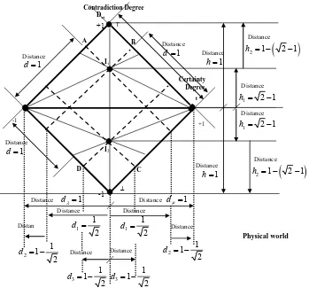
Figure 1. Correlation of values between the physical world and the Paraquantum universe represented by the lattice of the Paraquantum logics PQL.
2 1
h (9)
where: h is the Paraquantum Factor of quantization.
After the Superposed Paraquantum Logical state sup has reached the point where the Paraquantum logical state of quantization h is (which is identified with the
Paraquantum Factor of quantization h) a Paraquantum
Leap occurs. In this case, the module of the Vector of States P() is greater than one and the Real Certainty Degree will vary as follows:
1 h2 1
0.0823922
D
C R
D (10)
which will approximately be: C R . Each time the Superposed Logical states sup pass by the point that represents the Paraquantum logical state of quantization h, located on the vertical axis of contra-
diction degrees, it occurs a Paraquantum Leap that adds or subtracts the value of the Real Certainty Degree of the Leap.
Equation (11), which relates the Paraquantum logical states, shows that the Uncertainty Region of the PQL
depends on the transition frequency level N which acts on the Paraquantum Factor of quantization hψ such that:
1
2 2
N
IP
h
(11)
With: N a natural number equal or greater than 1. Where: ΔψIP = variation around the Paraquantum logi- cal state of Pure Indefinition.
N = frequency level of expansion or number of times of application of hψ.
With respect to the physical world the contraction of the Fundamental Lattice, which happens from the Paraq- uantum logical state of Pure Indefinition ψIP, has its val- ues given by:
Favorable evidence Degree: 1
2 2
N
N
h
Unfavorable evidence Degree: 1
2 2
N
N
h
where: N is a natural number equal or greater than 1 that indicates the transition frequency level of the Lattice.
1.3. The Fundamental Lattice of the PQL
The contraction of the Fundamental Lattice shows that a Paraquantum logical state ψ is a Fundamental Lattice infinitely contracted and has, through the Factor Paraq- uantum of quantization hψ, all features of the Fundamen- tal Lattice of the PQL [12,13]. These features can be de- termined not only for the Paraquantum logical state of Pure Indefinition ψIP but also for any point of the Lattice of the PQL.
2. The Paraquantum Logical Model for
Calculations of Values
Let QValue be a quantitative value of any physical quanti- ties such as: distance, displacement, speed, velocity, ac- celeration, force, mass, momentum, energy, work, power, etc. This value can be represented on the horizontal axis of certainty Degrees and on the vertical axis of contra- diction of the Lattice of the PQL. In the Paraquantum Logical Model [14,15]this maximum quantitative repre- sentation QValuemax corresponds to the distance from the
point, which is equidistant from the Vertices of the Lat- tice where the Paraquantum logical state of Pure Indefi- nition ψIP is, to one of the Vertices that represent the ex-
treme Paraquantum logical states of the Lattice. Consid- ering the maximum quantity QValuemax as an action of
contradiction, the relation will be the distance from the point equidistant of the Vertices of the Lattice to where the extreme Paraquantum logical states Inconsistent T or Undetermined . In this case, we can obtain on the Fun- damental Lattice of the PQL the relation between the Paraquantum Factor of quantization hψ and the quantita- tive value QValue of any physical quantities through the following:
max
Value Fund QValueh h Q
Q
(12)
where: Valueh is the value of the quantity on the Paraq- uantum logical state ψhψ.
max
Value Fund is the value of the total quantity repre- sented on the unitary axis of the Fundamental Lattice.
Q
1h 1 h
max maxFund Value Fund
Q h Q
h Q
Since the maximum value on the Fundamental Lattice of the PQL is normalized (equal 1), then we can write:
So, the unitary value of the quantization corresponds to a paraquantum quantization represented on the Paraq- uantum logical state ψhψ added to the value of its com- plement [14,15]. So, we have:
max
1
Value Fund Value
or since h 2 1 :
2 1max
max
1
2 1
maxValue Fund
Value Fund Value Fund
Q
Q Q
max max
max max 1
N
Value N Value N N
Value N Value N
Q h Q
Q h Q
(13)
The equations show that the maximum quantity of any physical quantities in the physical environment is com- posed of two quantized paraquantum fractions where one is determined on the Paraquantum Logical state of Quan- tization ψhψ by the Paraquantum Factor of quantization hψ, and the other is determined by its complement (1 − hψ). Applying the same process of quantization for frequency levels n = N, the values of quantization on the Paraquan- tum Logical model are given by:
or since h 2 1 :
max max
max max 1
2 1 2 1
N
Value N Value N
N
Value N Value N
Q Q
Q Q
(15)
for N a natural equal or greater than 1.
For the paraquantum analysis we observe that the maximum quantity of any physical quantities in the phy- sical world on the frequency N is composed of two quan-tized paraquantum fractions where:
a) one is determined on the Paraquantum logical state of Quantization ψhψby the Paraquantum Factor of quan- tization to the power of N such that(hψ)N;
b) the other is determined by its complement on the frequency N.
The relation to the axis can be obtained from the val- ues on the vertical axis of the contradiction degrees and from the values on the horizontal axis of the certainty de- grees.
The analysis of the quantities in the physical environ- ment is related to the values of Certainty Degree DC and Contradiction Degree Dct, both quantized through the Paraquantum Factor of quantization hψ (see [12,13]).
Quantization Factor of the Paraquantum Leap
Leap
t
h h h
Paraquantum logical states of quantization ψh defined in
infinitely many Local Fundamental Lattices in the Lattice of PQL [12,14,15].
ψh is a value added to or subtracted from the total quan-
tized value that appears at the instant of the Paraquantum Leap. So, in a relation where the quantity of the Large- ness in the physical environment is related to the Degree of Contradiction Dct, the value of the Real Certainty De- gree DCR is considered as a Factor of quantization in the Paraquantum Leap as seen in (10).
The propagation of the Superposed Paraquantum logi- cal states ψsup through the Lattice of the PQL causes the occurrences of Paraquantum Leaps that originate effects in the form of variations on the Real Certainty Degrees—
DCψR. The resulting value of this effect is added to or subtracted from the resulting value of the analysis, de- pending on if the considerations are being made as refer- ring to the “arrival” or to the “departure” of the propaga- tion. So, the value added to or subtracted from the Paraquantum Leap in the form of Real Certainty Degree—
DCψR depends on the Frequency level of the Lattice or the number of times of application of the Paraquantum Fac- tor of quantization hψ.
For a complete equationing the total Factor Paraquan- tum of Quantization in the Fundamental Lattice of the
PQL is expressed with the Factor related to the Paraq- uantum Leap, added to or subtracted from the Paraquan- tum Factor of quantization hψ, such as:
1 2 1
t
h h h
For the Fundamental Lattice the quantized value of the Real Certainty Degree—DCψR due to the Paraquantum Leap, which is added to or subtracted from, is computed by (11). Figure 2 shows the effect of the Paraquantum
Leap in the quantization of the values when the Super- posed Paraquantum logical states ψsup reach the point where the Paraquantum logical state of quantization ψhψ in the Lattice of the PQL.
We observe that in a quantitative relation the Real Certainty Degree—DCR produced in the Paraquantum Leap on the Paraquantum logical state of quantization
(16)
1 2 1
t
h h h
We have: a) is the Factor
Paraquantum of total Quantization at the “arrival” at the Superposed Paraquantum logical state ψsup, at the equi-librium point where the Paraquantum logical state of quantization ψhψ is.
1 2 1
t
h h h
b) is the Factor Paraquantum
of total Quantization at the “departure” from the Super- posed Paraquantum logical state ψsup, at the equilibrium
Physical world Measurements Observable
variable B
Physical world Measurements Observable
variable A Information
Source 2
Information Source 1
Certainty Degree Dc
λ 1 0 1 μ
-1 -1
t +1 +1
Contradiction Degree Dct
2)
P(ψ)F
Dc = 0
DC,R = ±0.0823922
MP(ψ)F = 1
P(ψ)t
Dct = hψ
MP(ψ)t = 1
hψFT h
ψtT
ψhψ
1 2 1
2 2
1 2 1
2 2
[image:5.595.140.454.421.709.2]
Figure 2. The Paraquantum Factor of quantization on the paraquantum logical state of quantization h due to Para-
point where the Paraquantum logical state of quantization ψhψ is.
For Lattices of the PQL with transition frequency lev-els N the equation of the Factor Paraquantum of total Quantization h is expressed as follows:
1
h2 N 1
Ntn N
h h (17)
with: a)
1 h2 N 1
Ntn N
h h the Factor
Paraquantum of total quantization at the “arrival” at the Superposed Paraquantum logical state ψsup, at the equi-librium point where the Paraquantum logical state of quantization ψhψN is.
b)
1 h2 N 1
max maxalue N N
Value N
Q
Q
Ntn N
h h is the Factor Pa-
raquantum of total quantization at the “departure” from the Superposed Paraquantum logical state ψsup, at the equilibrium point where the Paraquantum logical state of quantization ψhψN is.
With: N natural equal or greater than 1.
Using the above equation of the Paraquantum Quanti- zation, which relates values of quantities of physical largeness to the Lattice of the PQL, can be expressed by:
maxmax 1N Value N tn N V
tn N Value N
Q h
Q h
(18)
where: hψtn = N is the Factor Paraquantum of total Quanti- zation computed by:
1 h2 N 1
N tn N
h h (19)
We observe that hψtn=N adds the related Factor to the Paraquantum Leaps at the arrival at the propagated Paraquantum Logical states on the point N or subtracts the related Factor from the Paraquantum Leaps at the departure of the propagated Paraquantum Logical states on the point N.
3. Paraquantum Analyses in Physical
Systems
Based on the above equations we present the Paraquan- tum Logic (PQL) as a logical solution for resolution of phenomena modeled by the laws of Physics [5,11,16]. In order to develop this study, we start its application base on assumptions made from experimental observations of the Newton laws. Doing this the PQL will allow, through the Paraquantum Logical Model [14,15], the mathemati- cal applications to be extended to all fields of the physi- cal science.
In the application of the model based on the Paraq- uantum Logics PQL in resolution of physical phenomena, we would like to emphasize the importance of the second Newton law which expresses the crucial statement about how objects move when subject to forces [12].
The idea of the second Newton law is that when a re- sultant of forces acts on a body, this body will receive an acceleration which is proportional to Force (F) and in- versely proportional to its mass (m) [17,18]. When the law is expressed as a mathematical equation, this state- ment depends on a value that adjusts or defines this pro- portionality between the physical largenesses, such that:
1 or
F
a k F m a
m k
(20)
where:
a is the acceleration or the ratio through which the velocity of the body changes along time.
F is the resultant of all forces acting on the body.
M is the mass of the body.
k is a factor of adjustment of proportionality.
In order to apply the Paraquantum Logics PQL on physical systems it is important to study Newton’s laws which relate the involved physical largenesses (force,
mass and acceleration) with the British System of units as well as the implications with respect to their transfor- mations to the International System of Units (SI) [16,18]. In the British System of units those Physical largenesses considered fundamental are defined as: force, length and
time. Because of that there is no freedom to choose units for force and acceleration that must be used, however, to define the unit for mass so large or so small as desired. Doing so, the value of the proportionality constant k in (38), which represents the second Newton law [16], de- pends on the value of the unit chosen for mass. For the unit of force when the proportionality factor k acts on the
mass, where the force and the acceleration are 1 in the International System of units (SI), the equation that ex- presses the poundal of the British System [16-18] of units is expressed by:
2
1 pdl 32.174049 1 lbm. 1 ft
s
(21)
We repeat the above again but now using the corre- sponding values from the International System of units (SI) where the unit for force is the Newton (N). In this case, (39) can be expressed by:
2
1 N 4.448221615 1 Kg 1 m s (22)
The theoretical and experimental values show that the
PQL is a logic capable of creating models that can repre- sent the physical phenomena with a good approximation of the values obtained through the equations representing the second law of Newton. So, it is possible to adapt the factors of proportionality adjustment k obtained for the Paraquantum Logical Model as follows:
1.3825
br
k 4952 2
and
1 3951
2
N
0.723301
SI
k
Considering that the values of k were obtained from arbitrary measurements, whose values were adapted along the years with practical applications, the differ- ences are low.
3.1. The Newton Gamma Factor
This corresponds to the Paraquantum Factor of quantize- tion h obtained on the equilibrium point where the Paraquantum logical state of quantization h is lo- cated [12,13]. In the application of the Paraquantum Logical Model in broad areas of physics, the factor 2, as well as its inverse value, will be largely used to per- form adjustments needed to the natural proportionality that exists between physical quantities and adjustment of unitary values between unit systems. Due to its impor- tance, we will call this value Newton Gamma Factor and represent it by N. Therefore, for the classical logic applied in the Paraquantum Logical Model [14,15], we have Newton Gamma Factor N 2
P
.
3.2. The Paraquantum Gamma Factor
Equation (11) expresses the variation of the value of the Favorable evidence Degree µ extracted from measure- ments performed on Observable Variables in the physical environment, correlating to the Paraquantum Factor of quantization hψ on the lattice of the PQL.
When we consider obtaining the Favorable evidence Degree only, this equation can be written as follows:
1 1
2 N 2
incresc h
(23)
The condition previous to the analysis, which resulted
in 1
2
, can be mathematically expressed through
multiplications of inverse values of the Newton Gamma Factor [12,13]. In a procedure of expansion of the lattice, keeping the inverted value of the Newton Gamma Factor in the successive applications, we can identify the Lor- entz factor in the infinite series of the binomial ex- pansion. As was seen in [13] we identify a correlation
value of the paraquantum logics which we call Paraq- uantum Gamma Factor P such that:
1
P
N
(24)
where:
N
is the Newton Gamma Factor such that 1
2
N
is the Lorentz Factor.
Using the Paraquantum Gamma Factor P allows
the computations that correlate values of the Observable Variables to the values related to the quantization through the Paraquantum Factor of quantization hψ to be performed in any area of study of the physical science. The applications of the P can be done from relativity
theory to quantum mechanics.
3.3. The Applied Paraquantum Gamma Factor P
in the Paraquantum Logical ModelThe Paraquantum Logical Model is a way to study physical phenomena through the Paraquantum Logic
PQL based on measurements performed on Observable Variables in the physical environment. According to what we have seen so far, the analysis between the sys- tems of units and the adjustments with Newton’s laws which govern classical physics, produced the Newton Gamma Factor N 2 in the paraquantum analysis
[12,13].
3.4. The Variable Observable Velocity in the Primordial Lattice of PQL
In the so called uniform linear motion (ULM) there is no acceleration and the object being studied has constant velocity v [19-21]. For this condition, according to New- ton’s laws, the resulting of forces acting on the body is null. Given a displacement Δs during a measured time Δt the scalar velocity v is obtained by: v s
t
.
We observe that the concept of velocity or the physical state of movement in classical mechanics need two values established by measurements of two Observable Vari- ables in the physical environment and when we consider them from the PQL viewpoint we have:
1) Observable Variable time t which appears on the equation with the measured inverse value such that:
1
measured v
t
2) Observable Variable space s which appears on the equation with the value measured such that
1
peated actions of the application of the inverse value of the Newton Gamma Factor, the velocity is related to the Primordial Lattice of the Paraquantum Gamma Factor
P
, such that: 1
2
s v
t
.
This condition suggests values defined for a Primor- dial Lattice of paraquantum analysis where, at the time of obtaining de evidence Degrees from the physical envi- ronment for a fundamental unit of the Observable Vari- able s, there is a fundamental variation of the Observable Variable time flow t of 2. So, the primordial equation shows that for length 1 the velocity v of the body in rela- tion to the speed c of the light in the vacuum is repre- sented by the inverse value of the Newton Gamma Factor
P
. However, in this condition the velocity is not 1 but:
1 2
v .
Considering the equation of velocity only and analyz- ing through the concepts of PQL, we observe that this contradiction is produced by the time t when it is seen as an Observable Variable in the physical environment.
3.5. The Measured Time t Considered as Variable Observable
Time when considered as an Observable Variable in the physical environment which is able to produce Favorable and Unfavorable evidence Degrees µ or λ, respectively, for the paraquantum analysis, but produces a measure- ment with features different from other fundamental largenesses, such that its values always increase and never decrease, behave as a contradiction producing fac- tor.
Time, as expressed in the denominator of the equation of velocity is the fundamental largeness that produces in the Newton’s equations the need of the factor of propor- tionality adjustment and is represented in the paraquan- tum analysis by the Newton Gamma Factor N 2
We initially observe that for a Universe of Discourse (or Interest Interval), considered in the Paraquantum Analysis, the evidence Degree obtained from measure- ments of the Observable Variable time has the following properties:
.
1) measurements are necessarily quantized due to its fluidity.
2) its measured value always increases, never de- creases, which makes it to be considered a flow of posi- tive values.
3) in reality its value is never stable therefore can never be considered a constant.
The unit of time measured, in order to be considered as maximum Favorable evidence Degree in the Primordial Lattice of the PQL, is normalized and therefore following the condition imposed to the equation of velocity has
always the inverse value of the Newton Gamma Factor. So, considered in the Paraquantum Logical Model, the extraction of the evidence Degrees done through the Ob- servable Variable time produces a quantified value of its contribution to the value of the Observable Variable ve- locity, which always is, in the Newtonian universe; 1
2 .
However, since time is not unitary but shows a value of measured time similar to a flow of continuous increment, then when the Paraquantum Logical Model is effectively applied outside the Newtonian universe, the Observable Variable time receives action of the Paraquantum Gamma Factor P and produces contradiction in the analysis.
3.6. The Paraquantum Gamma Factor
P and the Measured Time tFirst we consider that the value of velocity v can also be represented by the measured space s
t
divided by the measured time . So, the equation of Lorentz Factor
can be expressed as follows:
2 2 2
1 1 1
1 1
1
v s s
c c
c t t
c
In a contraction of values in the paraquantum analysis the timet is linked to the space s to receive the action of the quantization frequency η by the repeated application of the inverse value of the Newton Factor N. The Pri- mordial Lattice, with its values established in the Newto- nian universe, relates time with the value of the Newton Gamma Factor N such that:
s v
t
1 1
2 N
(25)
In the Primordial Lattice the equation of velocity is expressed with the primordial values of largenesses such that:
1
1 . 1.
. 2
measured
v s
t
or
1
1 . 1.
.
measured N
v s
t (26)
medido N v v
2 1.
v 1 s
1 .
1 . 2
t
or after rewritten so that it becomes compatible with the expression of velocity of the laws of classical mechanics of the Newtonian universe:
1 .
N N
s
1
1 .
1 .
measured
v t
(27)
Considering that in the Newtonian universe the Paraquantum Gamma Factor is approximately equal to the inverse value of the Newton Gamma Factor N, the equation of the velocity in the Paraquantum Logical Model can be rewritten as follows:
P .
Ps
1 1 .
. measured
v
t
so the flow of paraquantum time is the time measured, quantified and its value is expressed by:
measured P
t t
t
(28)
where: measured = measured variation of time P
= Paraquantum Gamma Factor from (24).
The Equation (25) which deals with velocity can be written in the form where the action of the Paraquantum Gamma Factor can be visualized:
v 1
P measured P
s t
t
(29)
where: measured = measured variation of time. s
= measured space.
We also consider that the property of the fundamental physical largeness time has continuity of increment which means that it can never be zero.
4. The Paraquantum Physical Largenesses
Based on the considerations and equationings done with the foundations of the Paraquantum Logics PQL [12-15] we present the fundamental largenesses of Physics through the action of the quantization factors.
4.1. The Paraquantum Velocity v
The variation of the continuous increment of the value of
time, whose measured value affects the value of velocity, considers that, in the Paraquantum Logical Model, its Interest Interval may change by its own action. This means that time, in its representation in the Primordial Lattice of the PQL, forces the values of space s and, as a consequence, the value of velocity v, to be multiplied by the Newton Gamma Factor N when they are measured. We can introduce a concept of paraquantum velocity
such that from (29) we obtain:
P
measured P s v
t
v
(30)
= paraquantum velocity.
where: measured
t = measured variation of time.
= Paraquantum Gamma Factor. P
s = measured variation of space.
The paraquantum velocity is the representation of the velocity of the body which is considered as a physical state of motion in the PQL because it is represented by a Paraquantum Logical state ψ. So, paraquantum velocity is represented through the analysis by two evidence De- grees extracted from two Observable Variables in the physical environment: time t and traveled space s. Since the longer is the time measured in equal intervals of trav- eled space, the lower the velocity is, then for the proposi- tion P: “velocity is high”, the time represents the Favor- able evidence Degree [3,21-23] when it is received with the resulting inverse value such that:
Favorable evidence Degree: 1 measured P
t
Since the shorter is the space measured in equal inter- vals of constant time, the higher the velocity is, then for the same proposition P: “velocity is high”, the traveled
space represents the Unfavorable evidence Degree when it is received with the resulting inverse value such that: Unfavorable evidence Degree: sP.
According to the foundations of the PQL, in a dy- namical process the quantization of velocity will happen at the equilibrium point where the Paraquantum Logical state of quantization ψPψis, that is, in the state that ex- presses the action of the Paraquantum Factor of quantize- tion hψof the P QL. Equation (30) of velocity becomes the one of the quantization of the state of velocity and is obtained by:
P
tmeasured P s
v h
t
measuredP
P
1 2 1
sv h h
t
v
(31)
where:
= quantized value of the state of velocity or mo-
tion of the system. measured
t = measured time variation.
= Paraquantum Gamma Factor. P
s = measured traveled space variation.
h = Paraquantum Factor of quantization 2 1
. Writing:ss2s1 and t t t
2measured 1measured
2 1
2 1
P
measured measured P
s s
v
t t
2
1 1
h h (32)
where: s1 = measured initial space.
s2 = measured final space.
1measured t t
= measured time at the initial traveled space.
2measured
In the representation that expresses the value of state of velocity in the system, all performed measurements in the physical environment related to the Observable Variables time t and space s are multiplied by the value of the Paraquantum Gamma Factor
= measured time at the final traveled space.
P found in (24).
In the case of motion with velocity much lower than the speed of light in the vacuum, hence in the Newtonian universe, the inverse value of the Newton Gamma Factor
1
can be used due to its proximity to the value of the N
Paraquantum Gamma Factor P.
We observe that according to (32) for any value of measurement on Observable Variables in the physical environment, there is no contradiction with the basic laws of physics in the application of the Paraquantum Gamma Factor since the values of measured time and traveled space s are captured in a sequential way and it causes the annulment of the action of the Paraquantum Gamma Factor in the physical reality. However the rep- resentation in the Lattice is only possible by the action of the Paraquantum Gamma Factor on the measurements which produces the quantization of the state of velocity through the Paraquantum Factor of quantization hψ.
4.2. The Paraquantum Acceleration a
According to classical physics [18,22,23], in the study of the uniform linear motion (ULM) the object has constant velocity and the resultant of forces acting on the body is null. For these conditions given a displacement s dur-
ing time t, the scalar velocity v is given by: v s
t
.
Different from the ULM, in the uniformly varied linear motion (UVLM) the object being studied varies its ve- locity in a constant fashion, that is, the object has con- stant acceleration. So, the equation of acceleration is similar to the one of the velocity in the ULM which is:
v a
t
. In physical systems of this sort, acceleration
depends on the variation of velocity v in relation to the measure time t. Since force acting on a body causes the variation of velocity as well as changes in the mass, then acceleration depends on the force F applied to the body and on its mass [20]. However Force and mass can act independently in the system with respect to the applica- tions of force and variations of mass. In this relation be-
tween these two physical largenesses we observe that their values caused the inverse effect of varying velocity and as a consequence, the acceleration. If the mass of a body in motion increases, its velocity will decrease and if force is applied in the sense of the body’s motion, veloc- ity will increase.
For applications in the same sense of the motion we can consider that the force causes the increase of the variation of velocity. Therefore the values of displace- ment, velocity and force are directly proportional to ac- celeration. On the other hand, the value of mass meas- ured and the value of time measured are inversely pro- portional to acceleration. However, we observe that in the representation on the PQL, the variation of velocity is quantified through a Paraquantum logical state ψ pro- duced by the analysis of measure time t and displacement
s. As it was seen, time, when considered as an Observ- able Variable in the physical environment, has a special feature, namely, fluidity which is different from mass. However the measured time always has its value multi- plied by the Paraquantum Factor of quantization and it only affects the measurements when the value of velocity variation is high. Equation (30) expresses the paraquan- tum velocity and can be expressed as follows:
1
P measured P
s v
t
.
According to the laws of physics and using the previ- ous equation we can obtain the paraquantum acceleration by writing the following:
measured P v a
t
hence:
1
P measured P
v a
t
From (32) we can rewrite (31) as follows:
2 1
2 1
2
1
1
1 1
P measured measured
P
s s
v
t t
h h
2 1
2
1 1
1 1
P P
v V V h h
Taking the equation of the paraquantum acceleration to this last equality we have:
2 1 2
2 1 1
measured P
V V
a h h
t
a
(33)
where:
= quantized value of the state of acceleration of
the system.
2
1
V
measured
t
= value of the initial measured velocity. = measured time variation. = Paraquantum Gamma Factor. P
s = variation of the measured traveled space.
h = Paraquantum Factor of quantization
2 1
. We observe that according to (33) for any value of measurement on the Observable Variables in the physical environment in the Newtonian universe, there will be no contradiction of the basic laws of physics in the applica- tion of the Paraquantum Gamma Factor. This happens because the Paraquantum Gamma Factor in the Newto- nian universe is approximately the inverse of the Newton Gamma Factor that in the acceleration appears in its square, resulting in a denominator of the equation of ap- proximately 0.5.We observe that this value is very close to the part of the equation related to the Paraquantum Factor of quan- tization hψwhich is in the numerator of the equation.
4.3. The Observable Variable Force in the Paraquantum Analysis
Being the paraquantum acceleration a as expressed in (33) and following the concepts of the Paraquantum Lo- gics PQL, we observe that, due to the action of time on
velocity, the force F that appears on (20), which repre- sents Newton’s second law, will receive action of the Paraquantum Gamma Factor P.
As it was seen for the velocity, this equation in the Primordial Lattice of the PQL will be initially written as an inequality such that: 1 .
1 . P
F a
m
.
We verify that under this condition we have a natural inequality in (20) which represents Newton’s second law: this inequality happens because of inherent properties of the fundamental physical largeness time. In order to have the equality satisfied we must have the quantity of the physical largeness acceleration decreased by the action of the Paraquantum Gamma Factor P. Hence, the pre- vious inequality becomes an equality which is expressed by the following:
1
1 . P
F
a P
m
where:
1
P
a a
,
which is the expression of the paraquantum acceleration. Hence, in order to obtain the value of the acceleration in the physical environment, when we have the value of the paraquantum acceleration, the equation is expressed as follows:
1
P
a a
a
a
(34)
where: = value of the acceleration of the body being
studied related to the physical world.
= value of the acceleration of the body being
studied related to the Paraquantum world. P = Paraquantum Gamma Factor.
Hence, we have the equation of the paraquantum ac- celeration as follows:
F am
P
(35)
a
where: = quantized value of the state of accelera- tion of the system.
F = value of the Force applied to the body being studied.
P = Paraquantum Gamma Factor.
m = mass of the body being studied.
From (35), which expresses the value of paraquantum acceleration which involves force and mass, we can iso- late the Force F of the paraquantum analysis such that:
F P
m a FConsidering that the paraquantum value of Force is mass multiplied by the paraquantum acceleration, then having the value of the paraquantum Force, its value corresponding to the physical environment is given by:
1
FF (36)
a a
P
where: = value of the acceleration of the body being studied relates to the physical world.
= value of the acceleration of the body being
studied related to the paraquantum world. P = Paraquantum Gamma Factor.
Being Force obtained by (20) such that:
1P
F m a
Then using in this equation the expression of the Paraquantum acceleration of (33) we have:
2 1 2
3 1 1
measured P
V V
F m h h
t
This last equation can be rewritten in such a way the one of the Observable Variables may be represented with quantized values by the action of the Paraquantum Gamma Factor, such that:
2 1
2
1 1
1 1
P P measured P
V V
F m h h
t
(37)
largenesses quantized. Hence, for a value of Force F
equal to the measured value, that is, without receiving the action of the Paraquantum Gamma Factor, we have:
a) the measured value of the variation of velocity
2 1
V V V
t1measured
is multiplied by the inverse value of the Paraquantum Gamma Factor.
b) the measured value of time variation
2measured
t t
is multiplied by the value of
the Paraquantum Gamma Factor.
c) the value of the mass m of the body is multiplied by the inverse value of the Paraquantum Gamma Factor. Since we cannot change the features which are inherent to the fluidity of time and velocity is not directly a part of the second equation of Newton, then in (37) we still have the condition that the measured value of mass does not receive the action of the Paraquantum Gamma Factor. In this case, where we consider the value of the mass to be the measured one, the Paraquantum Gamma Factor is multiplied by the measured value of force.
4.4. The Paraquantum Average Velocity
For any sort of motion studied we consider the value of the measurement of distance of an object from its initial point is given by its average velocity (Vaverage) and the measured time t. Hence, this description can be ex- pressed by: s Vaverage t
0.5
.
We observe in this equation of traveled space that its value s is obtained through the interaction of two physi- cal largenesses where one of them is the average velocity (Vaverage)which in the paraquantum analysis is considered as an Observable Variable from which we extract an evidence Degree. However, according to the foundations of the Paraquantum Logic PQL, the average of values is an undefined situation where the evidence Degrees ex- tracted from the measurements performed on the Ob- servable Variables bring: Favorable evidence Degree: and Unfavorable evidence Degree: 0.5. We have that the value of the average velocity is already multiplied by the value corresponding to evidence De- gree of Indefinition of the Paraquantum analysis. Hence, the average velocity in the Paraquantum Logical Model has a value computed according to the laws of physics [18,20-22]. We have:
1 2
1 2
2 1
. 2
average
V V
V V
V V
average
However, in the Newtonian universe, inverse value of the Newton Gamma Factor is considered, so the equation of average velocity can be expressed in a paraquantum form as follows:
2 1 2
1
average
N
V V V
V
2
V
1
V
(38)
where: average = quantized value of average velocity which is equal to the value obtained by the laws of phys- ics.
= measured value of final velocity. = measured value of initial velocity.
= Newton Gamma Factor which is 2.
t t
P
4.5. The Observable Variable Traveled Space in the Paraquantum Analysis
Being timet considered as the other Observable Variable in the equation of space [17,21], it is also approached by the paraquantum analysis as it was studied in the previ- ous equations, hence: measured P .
The equation of traveled space can be written in a paraquantum fashion as follows:
2 1 2
1
measured P N
s V V t
(39)
Since the Paraquantum Gamma Factor in the Newto- nian universe is approximately equal to the inverse value of the Newton Gamma Factor such that:
1 1
2
P N
then the equation of traveled space can be written with the factors in the form of values such that:
1 2
1 1
2 measured 2
s V V t
(40)
From (33) that expresses the paraquantum acceleration and using the approximation of the Paraquantum Gamma Factor as being the inverse value of the Newton Gamma Factor (40), we have:
2
2 1 21
1 1
measured N
a V V
h h t
Isolating V2, we have:
2 1
2
2 1 1
measured
a t
V V
h h
(41)
Replacing this value of V2 in (40) of traveled space ∆s,
we have:
1 1
2
ψ
1
2 2 4 1 1 2
measured
measured
a t
V V
s t
h h
1
2
2 2 1
measured
a t
s V
h h
1 1
2
1 measured
t
2
1 2
2 1
measured measured
a t
s V t
h h
2
1 1
2 1
(42)
Going back to the value of the Paraquantum Gamma Factor, the equation of space which due to the use of
paraquantum largenesses expresses a paraquantum value producing it by:
2 1
2
ψ
1 1
2 2 1 1
measured measured P
s V t a t
h h
(43)
s
where:
1
V
= variation of space traveled obtained from paraquantum values.
Hence, being Force represented by (37), such that:
= measured value of initial velocity. P
= Paraquantum Gamma Factor. measured
t
a
= measured variation of time.
= value of acceleration of the body in study re-
lated to the paraquantum world.
h = Paraquantum Factor of quantization
2 1
. Where the equation of traveled space used in classical physics is established and the action of the Factors from the Paraquantum Logics PQL.The traveled space Δs when analyzed from the paraq- uantum viewpoint becomes a Physical Largeness consid- ered as an Observable Variable and the evidence Degrees are extracted from it. Hence, the space traveled which is computed by (43) is considered a paraquantum space in which, when its value is obtained, in order for it to be reported to the physical world, will have to be multiplied by the Paraquantum Gamma Factor. Hence, being ∆sψa value of traveled space obtained by (43), the equation to report the value of traveled space to the physical world is:
1
P
s s
(44)
where: s = variation of measured traveled space.
s
= variation of traveled space obtained through paraquantum values.
P
= Paraquantum Gamma Factor.
4.6. Impulse
It is important in the paraquantum analysis to study the equation of quantity of impulse caused by force or mass which makes an object to move such that the value of the variation of velocity is represented by the paraquantum quantification: IP F tmeasured P
.
2 1
2
1
1 P 1 1
P measured P
V V
F m h h
t
then the Impulse will be:
2
2 1 2
1
1 1
P
P
I m V V h h
Q mv
(45)
4.7. The Amount of Movement
In the analysis of Quantity of Motion the following equa-tion is used: . Being paraquantum velocity rep-resented by (32) such that:
2 1
2
2 1
1 1
P
measured measured P
s s
v h h
t t
Then the value of the quantity of motion is obtained by:
2 2 1 1
2
1 1
P measured measured P
m s s
Q h h
t t
(46)
5. The Energy Equations of Paraquantum
Logic (PQL)
Using the equations of the physical largenesses repre- sented in the paraquantum analysis, we present in the following the equations of energy which constitute the Paraquantum Logical Model in the analysis of Physical Systems.
5.1. Work and Kinetic Energy