U.S. State and Local Fiscal Policies and
Nonmetropolitan Area Economic
Performance: A Spatial Equilibrium
Analysis
Yu, Yihua and Rickman, Dan S.
12 March 2013
by
Yihua Yu
Renmin University of China Beijing, China 100872
yihua.yu@ruc.edu.cn
and
Dan S. Rickman Oklahoma State University
339 Business Building Stillwater, OK 74074
dan.rickman@okstate.edu
Abstract. Faced with declining economic bases, many nonmetropolitan areas increasingly have become concerned about their future economic viability. A crucial dimension of this concern is the balancing of the need to be cost-competitive in terms of lower taxes against the need for provision of valued government services. Using a spatial equilibrium framework, this study econometrically examines the nexus between U.S. state and local fiscal policies and
nonmetropolitan county growth in earnings and housing rents during the 1990s. The results suggest that state and local fiscal characteristics were important location determinants. Some characteristics could be clearly identified as having dominant firm profit effects while numerous others were identified as having household amenity effects. In addition, fiscal policies appeared to be more important for economic growth of nonmetropolitan counties which were remote from metropolitan areas than they were for counties adjacent to metropolitan areas.
Keywords: Regional Fiscal Policies; Rural Development; Spatial Equilibrium
1. Introduction
Dating at least as far back as Tiebout (1956) and Tullock (1971) state and local
governments have long been thought to use fiscal policy to promote economic growth. Faced
with declining resource-based industries and competition with low-cost producers worldwide,
many rural areas in the United States could be especially expected to be interested in using fiscal
policy to broaden their economic bases and stimulate growth. Yet, the economic declines
experienced in rural areas place stress on governmental services, putting rural governments in the
difficult position of balancing the demand for needed services with the desire to be
cost-competitive with their tax policies.
In a general review of regional tax studies, Bartik (1991) concludes there is a modest
negative relationship between the magnitude of most taxes and metropolitan and state growth.
On the other side of the ledger, in his review of the literature Fisher (1997) reported that some
government expenditures consistently have positive effects, particularly those on highway
transportation, though he found less support for education and safety expenditures. Helms (1985)
found that taxes used to finance transfer payments such as welfare expenditures reduced growth,
while those used to finance public services such as highways and education did not reduce
growth, suggesting that it was important to control for categories of public expenditures in
examining the effects of taxes.1 Dalenberg and Partridge (1995) found greater education
expenditures and lower taxes as stimulating metropolitan area employment growth. Brown,
Hayes and Taylor (2003) found that while some state and local expenditures more than offset the
negative effect of taxes, most did not. Brown and Taylor (2006) found that the net effect of the
size of state and local government changed over time, having negative effects on private sector
growth in the 1980s, but likely on balance maximizing private sector growth in the 1990s.2
1
In a meta-analysis of the studies examined by Bartik (1991), Goss (1995) concludes that studies which fail to control for public services understate negative tax effects.
2
Mixed evidence also has been reported for nonmetropolitan areas and for industries of
particular interest to rural areas. Henderson and McNamara (2000) found food manufacturing to
be sensitive to state and local tax burdens in the Corn Belt region. Goetz (1997) also found such
a relationship for food manufacturing establishment growth among all U.S. counties. Yet, for
nonmetropolitan counties in the lower 48 U.S. states, Lambert and McNamara (2009) did not
find any negative significant relationships between the property tax burden and the location of
various types of food manufacturing plants. Among nonmetropolitan Indiana counties, Rainey
and McNamara (1999) reported that manufacturing firms tended to avoid counties with relatively
high property tax rates. Monchuk et al. (2007) found that increased local tax burdens had a
negative impact on income growth in Midwest rural counties, as did state personal and corporate
income taxes. Hammond and Thompson (2008) found that human capital investment increased
per capita income growth in U.S. nonmetropolitan labor market areas, while public infrastructure
investment did not. Huang, Orazem, and Wohlgemuth (2002) found that local government
expenditures on public welfare and highways increased rural population growth in the Midwest
and South. They further found that the net effect of local government expenditures and taxes is
approximately zero, or slightly negative, on rural working-age populations.
Thus, consistent with the conclusion of Wasylenko (1997), the results continue to vary
widely across studies, making it difficult to understand the ways and extent state and local fiscal
policies influence economic activity. Given the inconclusive evidence and the continued interest
in the issue among policy makers, this paper examines the relationship between economic
growth in U.S. nonmetropolitan counties and state and local fiscal policies. Using U.S. Census
data we examine the effects of state and local fiscal policies on nonmetropolitan county earnings
and housing rents during the 1990s.
The analysis rests on the widely used spatial equilibrium approach of Roback (1982)
which was adopted for examination of state and local fiscal policies by Gyourko and Tracy
(1989; 1991) for U.S. metropolitan areas. A primary advantage of the spatial equilibrium
the tax policies mostly work through affecting firm profitability or household amenity
attractiveness of a region (Beeson and Eberts, 1987; 1989). 3 In addition to an overall assessment
for nonmetropolitan counties generally, we also examine sub-samples to determine whether state
and local fiscal policies matter less for nonmetropolitan counties which are not adjacent to
metropolitan areas (Rainey and McNamara, 2002).
The next section presents the basic spatial equilibrium model used in this study. Included
is a review of the metropolitan results of Gyourko and Tracy (1989; 1991) to illustrate the spatial
equilibrium channels through which fiscal policies can affect earnings and housing rents. In
addition to extending the Gyourko and Tracy studies to nonmetropolitan areas, we also expand
the framework to consider firm location effects of fiscal policies. Section 3 discusses the
empirical implementation of the model. Presentation and discussion of results follow in section
4. We find consistent evidence that the composition of state and local fiscal characteristics
significantly influence the location of households and firms. We also find fiscal characteristics to
be more important in nonmetropolitan counties which are not adjacent to metropolitan areas than
in those which are adjacent. Section 5 contains a brief summary and concluding statements.
2. Theoretical Framework
The theoretical framework follows the spatial general equilibrium approach of Roback
(1982) and Beeson and Eberts (1989). In this framework, spatial differentials in wages and land
rents are assumed to reflect capitalized equilibrium values of site specific characteristics to firms
and households. Among the site characteristics which distinguish the attractiveness of regions for
firms and households are the tax and expenditure policies of state and local governments
(Gyourko and Tracy, 1989; 1991; Brown, Hayes and Taylor, 2003; Brown and Taylor, 2006).
3
2.1 Basic Model
The model assumes an economy comprised of two optimizing representative agents: the
household and the firm. A representative household earns income from selling one unit of labor
and chooses amounts of a composite good (X),residential land (Lh), and site characteristics (s) so
as to maximize utility subject to a budget constraint:
max U X L s( , h; ) subject to w+ I = X + rLh (1)
where w and r represent the wage and land rental rates, respectively; I denotes nonlabor income
which is assumed to be independent of worker location (s). The above can be solved to obtain the
indirect utility function, which is assumed equal across regions in equilibrium because of perfect
mobility of households (Roback, 1982):4
V s r w
V( , ; ) (2) where Vw > 0, Vr < 0, and with the sign of Vs depending on whether s is an amenity or
disamenity.
A representative firm produces the composite good X according to a
constant-returns-to-scale production function in terms of labor and land: X(Lf, N; s), where Lf is land used in
production and N is the number of units of labor, and s operates as a profitability shifter. The
good is traded nationally without frictions and hence has normalized price equal to unity. For a
given quantity of X, the firm minimizes costs in choosing the quantities of land and labor.
Assuming perfectly mobile firms, costs are equalized across locations and set equal to the
normalized price of the traded good:
1 ) ; , (w r s
C , (3)
where Cw > 0, Cr > 0, while the sign of Cs depends on how s affects production costs.
Assuming that the values of all characteristics are capitalized into wages and land rents in
spatial equilibrium, the effects of site characteristics on wages and rents can be obtained by
differentiating Equations (2) and (3) and solving for dw/ds and dr/ds (Roback, 1982; Beeson and
4
Eberts, 1989).5 In equilibrium, site characteristics which are considered attractive (positive
amenities) by households increase land rents and decrease wages. Characteristics valued by firms
increase both land rents and wages. Thus, characteristics valued by both firms and households
unambiguously raise land rents, while the wage effect depends on whether the firm or household
effect dominates. Thus, in reduced form, wages and rents both are a function of the site-specific
characteristics.
As shown in Table 1, the combined pattern in wages and rents can be used to determine
whether the dominant effect of a location characteristic on the economy is related to firm
profitability or household amenities (Beeson and Eberts, 1987). A characteristic which raises
both wages and rents is interpreted primarily as profit enhancing. This can be seen in Table 1, for
example, where an attribute is profitable but does not have any household amenity value. Even if
the characteristic also makes an area more amenity-attractive, the net positive effect on wages
indicates that the profitability effect dominates the amenity effect. Contrarily, a characteristic
which reduces profitability reduces both wages and rents. If a characteristic increases land rents
but lowers wages we know there is a dominant amenity effect ― shown in Table 1 as a
characteristic which is amenity attractive but does not have any profitability effect. A
characteristic raising wages but lowering rents is interpreted as having a dominant negative
amenity effect. Whether a characteristic is household amenity attractive whatsoever is revealed
by the effect on the real wage. For example, higher housing rents and an absence of a nominal
wage effect indicates a positive household amenity effect. Similarly, a rise in wages but an
absence of a rent effect indicates a negative household amenity effect.
2.2 Spatial Equilibrium Fiscal Effects
Gyourko and Tracy (1989; 1991) recognized that state and local government taxes and
expenditures were among the characteristics which affected firm profitability and household
5
amenity attractiveness of an area and hence wages and housing rents. Less congestion on the
roadways, for example, can reduce transportation costs for firms and increase household utility.
Taxes and government services though may differentially affect households versus firms. We
review their findings below to illustrate fiscal policy channels of influence within the spatial
equilibrium framework.
In a reduced-form examination of wages across U.S. cities Gyourko and Tracy (1989)
reported that state and local fiscal conditions explained almost as much of the variation in wages
as did worker characteristics. The seven fiscal variables included three tax variables and four
government services variables. As a group, the seven variables were significant across various
model specifications.
Higher local and state income tax rates were associated with higher gross wages,
suggesting that workers needed to be compensated for higher taxes. Thus, local and state income
taxes could be thought of as reducing the household amenity attractiveness of the city. Higher
state corporate income taxes reduced wage rates, suggesting that corporate income taxes could
not be shifted forward onto consumers or backwards onto capital owners. This fits the model
above which contains a frictionless tradable good and perfectly mobile capital, in which higher
corporate income taxes reduce firm profitability, reducing labor demand and nominal wages.
Violent crime was positively associated with wages, suggesting it was a household disamenity.
Likewise, lower fire protection acted as a household disamenity, raising wages. An education
variable was insignificant.
Although the above wage results are broadly consistent with fiscal policies affecting
regional household amenity attractiveness, this can only be convincingly established by
examining both the wage and housing price effects of fiscal policy differentials and calculating
hedonic prices. Thus, Gyourko and Tracy (1991) examined the variation of both wages and
housing prices across U.S. cities. In calculating hedonic prices for fiscal policy attributes,
Gyourko and Tracy (1991) found that fiscal policy differentials were nearly as important as
characteristics examined included combined state and local income taxes, state corporate income
taxes, property taxes, and measures of police, fire, health, and education services.
The fiscal characteristics having the greatest household amenity value were police and
health services. However, the values were primarily reflected in lower wages as payments for
lower violent crime and more hospital beds, being insignificant in the housing price equation.
Fire protection also had a slightly positive household amenity effect. With both housing prices
and wages estimated to be significantly lower with greater fire protection, counter to
expectations, the results also suggested a dominant negative profitability effect ― an
interpretation not considered by the authors.6 Lower wages also were significantly associated
with better police protection. Education services were insignificant and had the wrong sign.
In terms of taxes, state and local income taxes exerted a negative household amenity
effect through a negative housing price effect and an absence of a significant effect on wages.
Thus, instead of higher gross wages as found in Gyourko and Tracy (1989), the negative amenity
effect of income taxes was found to be capitalized into lower housing values. Higher property
taxes significantly reduced housing values, and by assumption of the theoretical model, had no
effect on wages; thus property taxes were interpreted as a household disamenity. Higher
corporate income taxes were surprisingly found to be a positive amenity as they were associated
with significantly lower wages and higher housing prices. Given the unlikelihood that corporate
income taxes were shifted to nonresidents (consistent with the model above), the authors suggest
the variable may have been capturing unaccounted for agglomeration effects which were passed
on to residents in the form of higher housing prices.
2.3 Reduced-Form Equations
The framework above then indicates that wages and rents can be written as reduced-form
outcomes of the site specific characteristics, among which include state and local fiscal policies:
w = f(FISCAL, z) (4)
r = g(FISCAL, z), (5)
6
where FISCAL denotes a vector of state and local fiscal policies, and z denotes other site specific
characteristics such as the natural amenity attractiveness of the area. The fundamental
assumption is that the site characteristics are capitalized into wages and rents in equilibrium. The
pattern of relationships between the factor prices and the fiscal characteristics across space reveal
whether there are dominant household amenity or firm profitability effects, and also whether
there are significant household amenity effects which are not dominant.
3. Empirical Implementation
Corresponding to equations (4) and (5), reduced form econometric equations are specified
for both earnings and housing costs in U.S. nonmetropolitan counties (excluding counties in
Alaska and Hawaii). Nonmetropolitan counties simply are those not included in metropolitan
areas by the U.S. Census Bureau in 2000.7 The full sample consists of 1,998 counties, which we
also separate into two sub-samples according to the rural-urban continuum codes developed by
the Economic Research Service of the U.S. Department of Agriculture. The first sub-sample
contains 1,040 nonmetropolitan counties which are adjacent to a metropolitan area. The second
sub-sample contains 958 nonmetropolitan counties which are not adjacent to a metropolitan area.
A list of the variables and descriptive statistics for the full sample are provided in Table 2.
The change in the natural log of earnings for employed residents (EARN
) and the change
of the natural log of housing costs (HCOST
) over the period 1990 to 2000 are the two primary
dependent variables.8 Although our theory indicates that land rents should be examined, housing
costs should be a good proxy for land rents because spatial differences in quality-adjusted
residential housing prices primarily result from differences in the embedded land values (Davis
and Palumbo, 2008).
7
We follow the U.S. Bureau of Economic Analysis in merging independent cities with the surrounding county to form a more functional economic area (mostly in Virginia).
8
The variable HCOST is constructed as the log of weighted average median gross rent ($
per month) of owner and renter-occupied housing units for 2000 (Gabriel, Mattey and Wascher,
2003). For owner-occupied units, median housing prices are converted into imputed annual rent
using a discount rate of 7.85% (Peiser and Smith, 1985).9 The monthly average of this amount
along with the median monthly rent for the renter-occupied units, weighted by the shares of
owner- and renter-occupied houses, is our median housing cost variable.
Hence, in the full sample and the two sub-samples, for county i, located in state s, we
specify the econometric hedonic equations as:
0 1 2 3 4 5
W W W W W W W
is is is is is is is
EARN SFISCAL CFISCAL REG AMENITY DEMOG
(6)
0 1 2 3 4 5
R R R R R R R
is
is is is is is is
HCOST SFISCAL CFISCAL REG AMENITY STRUC
... (7)
The difference equations reflect an economy transitioning from one static equilibrium to another
in response to a change in one or more site characteristics (Dumais, Ellison and Glaeser, 2002;
Partridge and Rickman, 2010). Econometrically, a difference equation provides certain
advantages over an equation in levels. For one, there are circumstances where there are
consistent unobservable influences that bias the levels-based estimates. In differences we
implicitly control for county level fixed effects. The difference equation has an additional
advantage as it often reduces the severity of multicollinearity.
SFISCAL is a vector of state fiscal attributes which includes five categories of state level
tax revenues and seven categories of state level expenditure variables. For the state fiscal
variables, we calculate effective tax rates by dividing state and local government tax revenues
from individual income, sales, property, corporate income and other taxes by state personal
income. The categories of government services also are divided by state personal income and
include expenditures on highways, education (elementary and secondary), public safety (police
protection, fire protection, and corrections), public health and hospitals, environment (natural
resources, parks and recreation), housing (housing and community development, sewerage, and
9
solid waste management), and government administration (financial administration, judicial and
legal). CFISCAL is a vector of county fiscal variables all divided by county personal income,
including county property and sales taxes. These fiscal variables are obtained from the U.S.
Census Bureau’s Census of Government (COG). Hence, the vector SFISCAL
(CFISCAL
) is
defined as the value of SFISCAL (CFISCAL) in 2002 minus the same for1992.10
The REG vector includes several categories of dummy variables: Census division
dummies (Pacific is the omitted division) used to capture growth differences common to a census
division; and U.S. Department of Agriculture Economic Research Service (ERS) dummy
variables indicating whether a county historically is farming dependent, mining dependent, has
30% of its lands as federally-owned, or is a recreational county. Also included in the REG vector
are ERS rural-urban continuum dummy variables and a dummy variable reflecting whether the
county is located in a state possessing a right-to-work law. Thus, in addition to controlling for
county levels fixed effects through differencing, inclusion of these dummy variables controls for
common unobserved influences on growth.
Further, we introduce a vector of natural amenity attributes (AMENITY) that may affect
changes in earnings and housing costs. Natural amenity variables include the following
measures: the average temperature for January and July, respectively, the average number of
days with sunshine in January and the average humidity for July, the percentage of county area
that is covered by water; the topography score index. These amenity variables also are taken
from ERS (McGranahan, 1999). Although these variables are fixed over time, changing demands
for amenities can lead to persistent regional growth differences (Graves, 1980).
We control for the influence of population characteristics on earnings by including
demographic variables (DEMOG
) in equation (6). The DEMOG vector includes six age and five
racial composition variables, four education variables, the percentage of population that are
10
female, married, and had a linguistic isolation problem, respectively. Also we control for housing
characteristics by including several housing quality related variables (STRUC
) in equation (7).
The STRUC vector contains the median number of rooms in the structure, the age of housing
units, the shares of 1-5 bedrooms out of total rooms, the share of housing units that are mobile
homes, and the shares with complete plumbing and kitchen. The median number of rooms
indicates the size of the housing unit. The age differences in the housing units reflect the
differences in construction technology, type and efficiency of mechanical systems (for example,
heating and wiring) and the time over which the structure has been subject to normal wear and
tear (Galster, 1987).
One of our empirical concerns is that county labor and housing markets could influence
the local fiscal variables, indicating reverse causality. For example, the greater are home values
in a county the lower are the tax rates needed to generate revenues to finance governmental
programs. Alternatively, a struggling region may be more prone to cut taxes or spend money on
categories believed to be productive such as on highways. If this is the case, OLS estimates of
Equations (6)-(7) would be biased and inconsistent. Likewise, there may be common shocks
underlying the state fiscal variables and county earnings and housing prices, inducing statistical
endogeneity.
To overcome the potential endogeneity of the fiscal variables, instrumental variable (IV)
estimation is implemented. Instruments are needed which affect the outcome variables only
through the mechanism of the fiscal variables but are exogenous. Thus, we require variables that
are strongly correlated with SFISCAL
and CFISCAL
butuncorrelated with the error term.
Because of the difficulty in finding such instruments we use beginning-of-period (1992)
levels of the fiscal variables as instruments for the subsequent differences. In addition,
recognizing that the political system could affect the outcome of local fiscal policies, we also
include two voting behavior variables as instruments. For instance, Republican governments may
tend to favor low taxes and low spending while Democratic governments may tend to have
instruments the fiscal variables in 1992 values plus two additional political voting behavior
instruments. We use the percentage of votes cast for the Republican candidate in the 1972
presidential election (PRES_REP72) and the percentage of presidential election turnout in 1972
(PRES_TO72), using deep lags to mitigate endogeneity.
There are several tests of the IV regressions that we perform. First, to diagnose the
possible endogeneity of SFISCAL
and CFISCAL
, the Durbin-Wu-Hausman test is employed.
Second, we employ the Anderson canonical correlations likelihood ratio test to check the
relevance of the excluded instruments. A rejection of the null hypothesis indicates that the model
is identified and that the instruments are relevant. Third, we conduct the Anderson-Rubin
likelihood ratio test to check whether the endogenous variables are jointly statistically significant.
Lastly, we check the identification conditions for our instruments; i.e., we test whether the over
identification restrictions hold (Sargan, 1958).
Further, we conduct sensitivity analysis to assess the robustness of our results. First, we
exclude the demographic variables in the earnings equation and housing structure variables in the
housing cost equation because as aggregate measures the DEMOG
variable and STRUC
variables may be endogenous (Partridge et al., 2010, Rickman and Rickman, forthcoming).
Second, in sensitivity analysis we omit the state level variables (state fiscal variables, census
dummy variables, right-to-work dummy variable; ERS dummy variables) and replace them with
state fixed effects variables in the IV estimation to control for all possible state level growth
differences.
We estimate standard OLS and IV models in our base case analysis and not spatial
econometric models. We dothis because spatial autocorrelation tests have difficulty determining
whether spatial heterogeneity underlies the presence of spatial autocorrelation because of data
pooling or whether it is of the nuisance variety arising from arbitrary boundaries of the units of
analysis (McMillen 2003). We pool the data to obtain an average national effect and for
increased efficiency of the estimates. Corrections for spatial autocorrelation also involve
spatial process at hand and it is unlikely that the spatial dependence can be accurately captured
by a single parameter on the weight matrix (Pinske and Slade, 2010). This especially applies in
our setting where there are missing spatial observations because of the omission of metropolitan
counties from the full sample, and particularly for the sub-samples of nonmetropolitan counties
based on adjacency/non-adjacency to metropolitan areas.11 Spatial lag analysis likely suffers
from the reflections problem, making causal identification problematic (Pinske and Slade, 2010);
thus, spatial lag analysis is better suited for descriptively examining correlations among members
or for predictive purposes as are time lags in time series forecasting. Nevertheless, in sensitivity
analysis, we include weighted fiscal policy variables for neighboring counties and allow for
spatial clustering in errors to produce robust estimated standard errors.12
4. Results
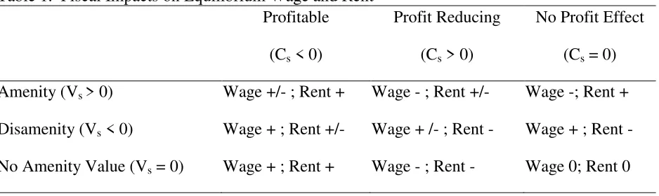
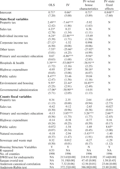
Table 3 contains the results from estimation of the housing rent growth regression
(Equation (7)) for the full sample, while Table 4 contains the corresponding results for earnings
growth (Equation (6)). The sole difference in specification of independent variables is the use of
population characteristic variables in the earnings equation and the use of housing characteristic
variables in the housing rent equation. In each table, the first column displays the results from
ordinary least squares (OLS) estimation. The second column displays the instrumental variable
(IV) estimation results using beginning-period levels of the fiscal variables and political voting
variables as the identifying instruments. IV estimates obtained after dropping the
housing/population characteristic variables appear in the third column. The final column of
results reflects the inclusion of state fixed effects to the IV column (2) model, while dropping all
county-invariant variables.
11
In a spatial hedonic application, Mueller and Loomis (2008) found that the potential inefficiency of OLS in the presence of spatially correlated errors was not economically significant, suggesting that nonspatial estimation was adequate. This may particularly be true in our setting because of the factors discussed above which make it problematic that efficiency can be improved with spatial estimation and may even be reduced.
12
From the first columns of results in Tables 3 and 4, the negative and significant effects
for state individual income taxes and the category of other state taxes for both housing rents and
earnings suggest dominant adverse firm profit effects. While personal income taxes could be
expected to raise the earnings of the employed to reflect household disutility, the negative firm
effect dominated to produce a net negative effect. This may particularly occur as owners of small
establishments pay personal income taxes and CEOs of larger companies may be influenced by
their personal income taxes in deciding where to locate their companies. The positive and
significant signs for state public safety expenditures in both equations suggest dominant positive
firm effects. Increased corporate incomes taxes are associated with significantly lower growth in
housing rents as are increased expenditures on government administration. State expenditures on
healthcare, and environment and housing, increased housing rent growth, which when combined
with insignificant earnings effects suggest household amenity attractiveness. Sales taxes have
unexpected positive signs in both equations. Sales taxes might be expected to increase earnings
as a disamenity but then housing rent growth also should be lower. The county fiscal variables
are generally insignificant, except for the significant negative sales tax effect on earnings growth.
More importantly, the IV estimates in the second column of Table 3 reveal significant
negative effects on housing rent growth from increased state property taxes, state individual
income taxes, and other state taxes. Combined with insignificant earnings effects (Table 4), this
suggests the taxes act as household disamenities. Increased state expenditures on highways, and
environment and housing are found to increase housing price growth, but have insignificant
effects on earnings, suggesting positive household amenity effects. Contrarily, negative housing
rent effects are found for increased expenditures on state education, health care and government
administration. State sales taxes and corporate income taxes are positively related to earnings,
though they are insignificant for housing rents, suggesting household disamenity effects. The
positive value for corporate income taxes is a surprise theoretically but empirically is consistent
with the findings of Gyourko and Tracy (1991). Significant positive effects on both housing rents
effects. Highway expenditures are negatively related to earnings and insignificantly related to
housing rents, suggesting household amenity attractiveness.
The instrument tests at the bottom of column (2) in Tables 3 and 4 suggest that the state
and county fiscal variables are statistically endogenous. Based on the Anderson canonical
correlation likelihood ratio tests the excluded instruments are relevant in both IV regressions and
the models are identified. The Anderson-Rubin likelihood ratio tests also indicate that the
endogenous variables are jointly significant in each equation. However, we reject that the over
identification restrictions hold in each regression.
As shown in column (3) of Tables 3 and 4, dropping the housing characteristic variables
from Equation (6) and the demographic variables from Equation (7) hardly affects the IV results.
A few variables slightly lose statistical significance in the two equations, while a few slightly
gain statistical significance. This suggests that coefficient bias from potential endogeneity of the
housing and population characteristics is not a major concern.
The final columns of results in both tables reflect the addition of state fixed effects and
the omission of all county-invariant variables (using the column 2 base model). State fixed
effects control for unmeasured state level influences on growth in housing rents and earnings.
The advantage of including state growth fixed effects is the reduction in possible omitted
variable bias in estimating the county fiscal policy effects. The disadvantage is the loss of
information on state level fiscal policy effects.
The Durbin-Wu-Hausman test suggests that the county fiscal variables are endogenous.
The tests also indicate that the models are identified and the endogenous variables are
significant. In contrast to the other IV models containing state fiscal variables, the over
identification restrictions hold in each equation at the five percent level.
Consistent with expectations of property taxes being capitalized into land prices (Brown,
Hayes and Taylor, 2003), county property taxes significantly and negatively influence housing
rents but have no significant effect on earnings, suggesting a household disamenity effect.
primary and secondary education and public safety have positive firm profitability effects. This
suggests that counties need to worry more about their provision of public safety and education
services to remain economically competitive in attracting firms than on lower sales taxes. In fact,
the positive effect of public safety on housing rents exceeds the negative effect of property taxes.
Highway expenditures have only a significant negative effect on earnings, and a positive
insignificant effect on housing rents, suggesting a positive household amenity effect ― but not
one that is dominant statistically.
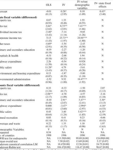
We next examine whether nonmetropolitan counties which are adjacent to metropolitan
areas respond differently to fiscal policy changes than those which are not adjacent (Rainey and
McNamara, 2002), though we continue to include dummy variables for the ERS rural-urban
continuum county categories which pertain to the specific sub-sample. The results for the two
sub-samples for both earnings and housing rents for the base IV model (column 2 model in
Tables 3 and 4) are shown in Table 5.
The base model instrumental variable evidence suggests fewer fiscal policy effects in
nonmetropolitan counties adjacent to metropolitan areas relative to counties not adjacent to
metropolitan areas. For metro-adjacent counties, only other state taxes have dominant negative
firm effects. Corporate income taxes again have the unexpected positive earnings effect (i.e., a
household disamenity effect). Negative expenditure effects on housing rents occur for state
primary and secondary education and government administration, while positive effects on
housing occur for expenditures on environment and housing. No significant county fiscal policy
effects are found.
Contrarily, for nonadjacent counties increased state property, individual income, and other
taxes lower growth in housing rents, as do increased county sales taxes, in which combined with
an absence of significant earnings effects suggests they are household disamenities. Increased
state expenditures on highways and public safety increase housing rent growth, suggesting
household amenity attractiveness, while expenditures on hospitals and health decrease growth.
rents) and highways (through lowering earnings) are revealed as positive household amenities.
The near significance of the earnings effect of county education expenditures suggests a strong
profitability role as well.
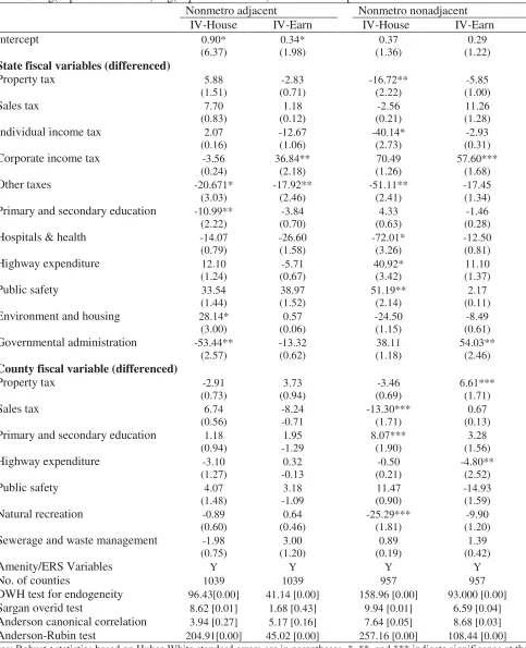
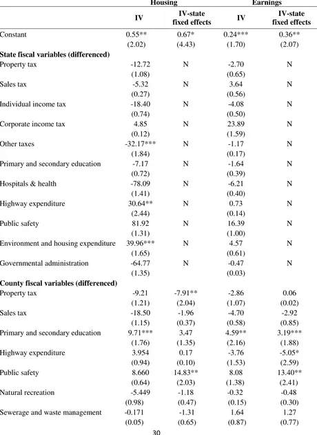
In final sensitivity analysis, Table 6 shows the results of adding variables reflecting
neighboring county fiscal variables and adjusting the standard errors for potential clustering of
the residuals. Neighboring counties are defined according to Bureau of Economic Analysis labor
market regions, which are defined as groups of counties with tight commuting links. Each
county’s fiscal variable is weighted by its share of population in the region minus the county
under study.13 Results for both the IV base model and IV state fixed effects models are presented
in Table 6.
The instrument tests at the bottom of column (2) in Table 6 suggest that the state and
county fiscal variables are statistically endogenous (at the eight percent level in column (2)).
Based on the Anderson canonical correlation likelihood ratio tests the excluded instruments are
relevant in both IV regressions and the models are identified (only at the 12 percent level in
column (4)). The Anderson-Rubin likelihood ratio tests also indicate that the endogenous
variables are jointly significant in each equation. Each equation passes the over identification
restrictions test at the five percent level.
The base model IV results suggest that the category of other state taxes acted as a
household disamenity. State expenditures on highways and on the category of environment and
housing acted as a household amenity. The county level results confirm the results in Tables 3
and 4 for the IV base model and the IV state fixed effects model. The IV state fixed effects
results suggest that county property taxes acted as a household disamenity. County level primary
and secondary education expenditures statistically enhanced county productivity according to the
base model IV results and nearly so according to the IV state fixed effects results. These
productivity effects dominated any possible amenity effects, to increase both earnings and
13
The Cluster Command in STATA is used for estimation. Comparable results are not reported for the adjacent and non-adjacent counties separately because labor market regions contain both types of counties, which make
housing costs. Dominant productivity effects for public safety also are evidenced in the IV state
fixed effects results.
Regarding the neighboring county fiscal variables, neighboring county expenditures on
primary and secondary education statistically reduce county productivity according to the IV
base model. Similar negative effects are found in the IV state fixed effects model, though the
effects are less precisely estimated. Thus, greater education expenditures in nearby counties
appear to draw firms away from the county, creating backwash effects. Higher sales taxes in
nearby counties produce negative productivity effects, possibly through reduced demand
(spread) effects. Higher neighboring county property taxes act as a household amenity,
suggesting that within labor market areas households avoid counties with higher property taxes.
5. Summary and Conclusion
Using a spatial equilibrium framework this study econometrically examined
nonmetropolitan county growth in earnings and housing rents for the 1990s. Consistent evidence
was found to suggest that state and local fiscal characteristics were important firm and household
location determinants. Contributions of the study include the application of the approach to the
study of nonmetropolitan areas and consideration of both household and firm effects. Some
characteristics could be clearly identified as having dominant firm profit effects while numerous
others could be identified as having household amenity effects.
Focusing on the primary instrumental variable evidence for the full sample, state
individual income, property, and other, taxes significantly discouraged growth through negative
effects on household amenity attractiveness. In terms of state government expenditures, those on
highways, and the environment and housing, could be identified as household amenity attractive.
Yet, consistent with the review findings of Fisher (1997) negative household amenity effects
were found for state education expenditures, as well as for expenditures on governmental
administration. The education findings may be attributable to the spatial pattern of education
spending in the state, rather than negative effects of spending in the county. The surprising
and Tracy (1991) for metropolitan areas, though is inconsistent with the negative relationship
often found in the literature (Felix, 2009).
Nevertheless, consistent dominant positive effects on firm profitability were found for
county expenditures on primary and secondary education. Some evidence also was provided
suggesting dominant firm profit effects from county spending on public safety. Consistent
evidence also was found for positive household amenity effects from county highway spending.
There was evidence of negative household amenity effects from increased county property taxes.
The positive effects of expenditures sometimes exceeded the negative property tax effects,
producing a net positive effect. We also found that fiscal characteristics were more important in
nonmetropolitan counties which are not adjacent to metropolitan areas than in those which are
adjacent. Most state and county taxes have negative household amenity effects in nonadjacent
counties, while county expenditures on education and state expenditures on public safety were
household amenity attractive.
Overall, the results suggest that policy makers should be concerned with being
cost-competitive with certain taxes, though they also should be careful to be cost-competitive in providing
local education and other valued government services. Future research should more fully explore
the contexts in which various mixes of fiscal policies promote economic growth. In addition,
after the release of Census 2010 summary file data it can be determined whether the importance
of state and local policies changed during an increasingly globalized economic environment and
national stagnation of employment growth.
References
Bartik, Timothy J. 1991. Who Benefits From State and Local Economic Development Policies? Kalamazoo: W. E. Upjohn Institute.
Bayer, Patrick, Nathaniel Keohane and Christopher Timmins, 2009. “Migration and Hedonic Valuation: The Case of Air Quality,” Journal of Environmental Economics and Management
58(1), 1-14.
_____, 1989. “Identifying Productivity and Amenity Effects in Interurban Wage Differentials,”
The Review of Economics and Statistics 71(3), 443-452.
Blanchard, Olivier, and Lawrence F. Katz, 1992. “Regional Evolutions,” Brookings Papers on Economic Activity 1-75.
Brown, Stephen P.A., and Lori L. Taylor, 2006. “The Private Sector Impact of State and Local Government,” Contemporary Economic Policy 24(4), 548-562.
Brown, Stephen P.A., Kathy J. Hayes, and Lori L. Taylor, 2003. ‘‘State and Local Policy, Factor Markets and Regional Growth,’’ Review of Regional Studies, 33(1), 40–60.
Dalenberg, Douglas R. and Mark D. Partridge, 1995. “The Effects of Taxes, Expenditures, and Public Infrastructure on Metropolitan Area Employment,” Journal of Regional Science 35(4), 617-640.
Davis, Morris A. and Michael G. Palumbo, 2008. “The Price of Residential Land in Large U.S. Cities,” Journal of Urban Economics 63(1), pp. 352-84.
Deskins, John and Brian Hill, 2010. “State Taxes and Economic Growth Revisited: Have Distortions Changed?”Annals of Regional Science 44(2), 331-348.
Dumais, Guy, Glenn Ellison, and Edward L. Glaeser. 2002 “Geographic Concentration as a Dynamic Process,” TheReview of Economics and Statistics 84: 193-204.
Felix, R. Alison, 2009. “Do State Corporate Income Taxes Reduce Wages?” Federal Reserve Bank of Kansas City Economic Review 94(2), 77-102.
Fisher, Ronald C. 1997. “The Effects of State and Local Public Services on Economic Development” New England Economic Review, 53-82.
Gabriel, Stuart A., Joe P. Mattey and William L. Wascher, 2003. “Compensating Differentials and Evolution in the Quality of Life among U.S. States,” Regional Science and Urban
Economics 33, 619-649.
Galster, George C. 1987. Homeowners and Neighborhood Reinvestment. Durham, NC: Duke University Press.
Goetz, Stephan J., 1997. “State- and County-Level Determinants of Food Manufacturing Establishment Growth: 1987-93,” AmericanJournalofAgriculturalEconomics 79(3), 838-50.
Goss, Ernie P., 1995. “The Effect of State and Local Taxes on Economic Development,”
Southern Economic Journal 62(2), 320-333.
Graves, Phillip, 1980. “Migration and Climate,” Journal of Regional Science 20(2), 227-37.
Gyourko, Joseph and Joseph Tracy, 1989. “The Importance of Local Fiscal Conditions in Analyzing Local Labor Markets,” Journal of Political Economy 97(5), 1208-1231.
_____, 1991. The Structure of Local Public Finance and the Quality of Life. Journal of Political Economy 99(4), 774-806.
Metropolitan and Nonmetropolitan Labor Markets,” American Journal of Agricultural Economics 90(3), 517-542.
Helms, L. Jay, 1985. “The Effect of State and Local Taxes on Economic Growth: A Time-Series Cross Section Approach,” The Review of Economics and Statistics 67(4), 574-82.
Henderson, Jason R. and Kevin T. McNamara, 2000. “The Location of Food Manufacturing Plant Investments in Corn Belt States,” Journal of Agricultural and Resource Economics 25(2), 680-97.
Huang, T.-L., P.F. Orazem, and D. Wohlgemuth, 2002. “Rural Population Growth, 1950–1990: The Roles of Human Capital, Industry Structure, and Government Policy.” American Journal of Agricultural Economics 84(3), 615–27.
Lambert, Dayton M. and Kevin T. McNamara, 2009. “Location Determinants of Food
Manufacturers in the United States, 2000-2004: Are Nonmetropolitan Counties Competitive?”
Agricultural Economics 40, 617-630.
Laurent, Héléne, Michel Mignolet and Olivier Meunier, 2009. “Regional Policy: What is the Most Efficient Instrument,” Papers in Regional Science 88(3), 491-507.
McGranahan, David A., 1999. “Natural Amenities Drive Rural Population Change,” Economic Research Service, U.S. Department of Agriculture, Washington, DC, AER 781.
McMillen, Daniel P., 2003. Spatial Autocorrelation or Model Misspecification? International Regional Science Review 26: 208-17.
Monchuk, Daniel C., John A. Miranowski, Dermot J. Hayes and Bruce A. Babcock, 2007. “An Analysis of Regional Economic Growth in the U.S. Midwest,” Review of Agricultural
Economics 29(1), pp. 17-39.
Mueller, Julie M. and John B. Loomis, 2008. “Spatial Dependence in Hedonic Property Models: Do Different Corrections for Spatial Dependence Result in Economically Significant Differences in Estimated Implicit Prices,” Journal of Agricultural and Resource Economics 33(2), 212-31.
Partridge, Mark D., Dan S. Rickman, Kamar Ali, and M. Rose Olfert, 2009. “Agglomeration Spillovers and Wage and Housing Cost Gradients across the Urban Hierarchy,” Journal of International Economics 78(1), 126-140.
_____, 2010. "Recent Spatial Growth Dynamics in Wages and Housing Costs: Proximity to Urban Production Externalities and Consumer Amenities," Regional Science and Urban Economics, 40 (6), 440-452.
_____, 2011. “Dwindling U.S. Internal Migration: Evidence of Spatial Equilibrium?,” unpublished manuscript.
Peiser, Richard B. and Lawrence B. Smith, 1985. “Homeownership Returns, Tenure Choice and Inflation,”American Real Estate and Urban Economics Association Journal 13(4), 343-360. Pinske, Joris and Margaret E. Slade, 2010. “The Future of Spatial Econometrics,” Journal of Regional Science 50(1), 103-117.
_____, 2002. “Tax Incentives: An Effective Development Strategy for Rural Communities?”
Journal of Agricultural and Applied Economics 34(2), 319-25.
Rickman, Dan S. and Shane D. Rickman, forthcoming. "Population Growth in High Amenity Nonmetropolitan Areas: What's the Prognosis," Journal of Regional Science.
Roback, Jennifer 1982. “Wages, Rents, and the Quality of Life,”Journal of Political Economy 90(6), 1257-1278.
Sargan, James 1958. “The Estimation of Economic Relationships Using Instrumental Variables,”
Econometrica 26(3), 393-415.
Tiebout, Charles M., 1956. “A Pure Theory of Local Expenditures,” Journal of Political Economy 64(1), 416-24.
Tullock, Gordon, 1971. “Public Expenditures as Public Goods,” Journal of Political Economy
79(5), 913-8.
Table 1. Fiscal Impacts on Equilibrium Wage and Rent
Profitable Profit Reducing No Profit Effect
(Cs < 0) (Cs > 0) (Cs = 0)
Amenity (Vs > 0) Wage +/- ; Rent + Wage - ; Rent +/- Wage -; Rent +
Disamenity (Vs < 0) Wage + ; Rent +/- Wage + /- ; Rent - Wage + ; Rent -
No Amenity Value (Vs = 0) Wage + ; Rent + Wage - ; Rent - Wage 0; Rent 0
Table 2. Variable Definitions and Descriptive Statistics
Variable Description Source Mean Std.
Dev. Dependent Variables
ln(earning2000) Log of annual earnings (in dollars) in 1999 for the employed
over 16 2000 Census 9.819 0.142
ln(earning1990) Log of annual earnings (in dollars) in 1989 for the employed
over 16 1990 Census 9.647 0.188
ln(housing2000)
Log of weighted average median gross house rent ($/month) of owner and renter occupied housing units in 2000 using shares of owner and renter occupied houses.
2000 Census 6.156 0.316
ln(housing1990)
Log of weighted average median gross house rent ($/month) of owner and renter occupied housing units in 1990 using shares of owner and renter occupied houses.
1990 Census 5.731 0.302
County Fiscal Variables (differences in shares of personal income 2002-1992)
Ctyproperty Revenue from property tax 1992/2002 COG 0.001 0.016
Ctysales Revenue from sales tax 1992/2002 COG 0.001 0.003
Ctyhighway Expend. on highway - charges on highway 1992/2002 COG 0.000 0.007 Ctysafety Expend. on public safety (police + fire protection) 1992/2002 COG 0.001 0.004
Ctynaturalrec Expend. on natural resource and parks recreation -
corresponding charges 1992/2002 COG 0.001 0.005
Ctysewerage Expend. on sewerage and waste management - corresponding
charges 1992/2002 COG 0.000 0.004
Ctyeducation Expend. on first and secondary education 1992/2002 COG 0.009 0.019 State Fiscal Variables (differences in shares of personal income 2002-1992)
Stl_property Revenue from property tax 1992/2002 COG -0.001 0.004
Stl_sales Revenue from sales tax 1992/2002 COG 0.001 0.003
Stl_rest Revenue from selective, license, and other taxes 1992/2002 COG -0.001 0.003 Stl_individual Revenue from individual income tax 1992/2002 COG 0.002 0.003 Stl_corporate Revenue from corporate income tax 1992/2002 COG -0.001 0.001
Stl_firstsecond Expend. on elementary & secondary education 1992/2002 COG 0.003 0.004 Stl_hospitalhealth Expend. on hospitals - corresponding charges 1992/2002 COG 0.000 0.002 Stl_highway Expend. on highway - corresponding charges 1992/2002 COG 0.001 0.002
Stl_publicsafety
Expend. on public safety (police, fire, correction, etc) -
corresponding charges 1992/2002 COG 0.002 0.001
Stl_environhousing
Expend. on natural resources, parks recreation., housing and community development, sewerage, solid waste management - corresponding charges
1992/2002 COG 0.000 0.002
Stl_govtadmin
Expend. on government administration (Financial
administration + Judicial and legal + General public buildings + Other_governmental administration)
1992/2002 COG 0.001 0.001
Demographic Variables (differences 2000-1990)
Married Percent population(15 years over) that are married 1990/2000 Census 0.119 0.029 Female Percent population that are female 1990/2000 Census -0.006 0.015
Disability Percent Civilian non-institutionalized population 16 to 64
Hispanic Percent population Hispanic 1990/2000 Census 0.016 0.028
Highschool Percent population 25 years and over that are high school
graduates 1990/2000 Census 0.133 0.036
Somecollege Percent population 25 years and over that have some college
degree 1990/2000 Census 0.100 0.025
Associate Percent population 25 years and over that have an associate
degree 1990/2000 Census 0.022 0.012
Bachelor Percent population 25 years and over that are 4-year college
graduates 1990/2000 Census 0.046 0.021
Age7_17 Percent population 7-17 years 1990/2000 Census -0.005 0.015
Age18_24 Percent population 18-24 years 1990/2000 Census -0.001 0.014
Age25_54 Percent population 25-54 years 1990/2000 Census 0.015 0.017
Age55_59 Percent population 55-59 years 1990/2000 Census 0.006 0.008
Age60_64 Percent population 60-64 years 1990/2000 Census -0.002 0.008 Age65up Percent population over 65 years 1990/2000 Census -0.002 0.016 Housing Characteristics (differenced 2000-1990)
House age Age of housing unit in (years) 1990/2000 Census 5.812 3.244
Share1bed Share of 1 bedroom house to total rooms 1990/2000 Census 0.003 0.018 Share2bed Share of 2 bedroom house to total rooms 1990/2000 Census -0.020 0.029 Share3bed Share of 3 bedroom house to total rooms 1990/2000 Census 0.008 0.030 Share4bed Share of 4 bedroom house to total rooms 1990/2000 Census 0.006 0.019 Share5bed Share of 5 bedroom house to total rooms 1990/2000 Census 0.001 0.010 Sharemobile Share of mobile units to all housing units 1990/2000 Census 0.014 0.036 Shareplumb Share with complete plumbing facility 1990/2000 Census 0.002 0.023 Sharekitchen Share with complete kitchen facility 1990/2000 Census -0.003 0.022 Amenity Variables
TempJan Mean temperature for January, 1941-71 ERS, USDA 31.476 12.279
SunJan Mean days of sunshine for January, 1941-71 ERS, USDA
153.10
3 33.639
TempJul Mean temperature for July, 1941-70 ERS, USDA 75.560 5.623
HumidJul Mean relative humidity for July, 1941-71 ERS, USDA 54.184 14.873
Topography Topography score ranging from 1-21, where 1 represents flat
plain and 21represents most mountainous land ERS, USDA 9.109 6.634
Waterpct Percent of county area covered by water ERS, USDA 3.466 9.757
Other Dummy Variables
Census_division Census Division Dummy Variables 1-9 ERS, USDA 5.237 1.886
RTW2 Right to work law dummy variable NRTW 0.560 0.497
Table 3. Dependent Variable: log(median house rent 2000)-log(median house rent 1990) for full sample of nonmetropolitan U.S. counties
OLS IV
IV-w/out house characteristics IV-state fixed effects
Intercept 0.71* 0.66* 0.71* 0.848**
(7.20) (5.00) (5.89) (7.60)
State fiscal variables (differenced)
Property tax 2.49** -7.44*** -5.92 N
(2.42) (1.86) (1.63)
Sales tax 4.23* 8.23 6.36 N
(2.78) (1.34) (1.11)
Individual income tax -6.24* -22.86*** -15.69 N
(5.39) (1.71) (1.56)
Corporate income tax -27.12* -1.52 0.998 N
(6.50) (0.08) (0.06)
Other taxes -7.55* -25.66* -27.02* N
(5.01) (4.25) (4.99)
Primary and secondary education 0.67 -6.86*** -9.94* N
(0.63) (1.68) (2.83)
Hospitals & health 3.39*** -53.085** -38.91** N
(1.72) (2.16) (2.25)
Highway expenditure -0.95 27.98* 30.18* N
(0.65) (5.08) (6.07)
Public safety 8.47** 33.46 19.04 N
(2.47) (1.56) (1.16) Environment and housing
expenditure
9.55* 22.44* 16.85** N
(5.25) (2.91) (2.49)
Governmental administration -17.06* -30.90** -14.01 N
(5.71) (2.05) (1.13)
County fiscal variables
(differenced) differences) (in
Property tax 0.34 2.35 2.64 -5.65*
(1.13) (0.68) (0.94) (2.73)
Sales tax -0.42 -9.12 -2.65 -0.027
(0.30) (0.96) (0.38) (0.01)
Primary and secondary education -0.13 3.85*** 3.26*** 2.66**
(0.56) (1.75) (1.77) (2.45)
Highway expenditure -0.14 -0.38 -0.77 0.16
(0.24) (0.25) (0.59) (0.17)
Public safety -0.072 -1.54 -1.69 8.65*
(0.07) (0.34) (0.45) (3.00)
Natural recreation -0.18 -2.94 -3.43*** -1.40
(0.37) (1.47) (1.91) (0.95)
Sewerage and waste mgt 0.32 0.012 -0.27 -1.29
(0.50) (0.01) (0.17) (1.12)
Housing Structure Variables Y Y N Y
R-squared 0.53 NA NA NA
No. of counties 1998 1996 1996 1996
DWH test for endogeneity NA 213.63[0.00]
[0.000]
218.93 [0.00] [0.000]
37.44[0.00] [0.000]
Sargan overid test NA 31.19[0.00]
[0.000]
47.45 [0.00] 1.58 [0.45] Anderson canonical correlation
LM test for relevance
NA 7.32 [0.06] 12.56 [0.01] 23.66 [0.00]
Anderson-Rubin test NA 372.23[0.00]
[0.000]
386.88[0.00] [0.000]
Table 4. Dependent Variable: log(earnings 2000)-log(earnings 1990) for full sample of nonmetropolitan U.S. counties
OLS IV
IV-w/out demographic
variables
IV- state fixed effects
Intercept -0.01 0.28* 0.10 0.43*
(0.13) (2.95) (1.09) (3.40)
State fiscal variable (differenced)
Property tax 0.87 1.33 1.55 N
(0.93) (0.48) (0.55)
Sales tax 3.64* 8.73** 7.41*** N
(2.62) (2.01) (1.66)
Individual income tax -3.48* -7.14 -9.85 N
(3.42) (1.14) (1.26)
Corporate income tax 5.13 23.73** 24.04*** N
(1.43) (1.97) (1.80)
Other taxes -4.69* -1.54 -2.43 N
(2.91) (0.35) (0.58)
Primary and secondary education -0.19 -2.27 -1.20 N
(0.19) (0.88) (0.44)
Hospitals & health -0.31 -2.68 1.94 N
(0.18) (0.22) (0.14)
Highway expenditure 2.26 -0.54 0.928 N
(1.59) (0.14) (0.24)
Public safety 11.28* 4.79 -3.61 N
(3.43) (0.37) (0.28)
Environment and housing expenditure 0.13 -1.87 -5.80 N
(0.07) (0.35) (1.10)
Governmental administration -2.52 9.52 18.47*** N
(0.96) (1.00) (1.92)
County fiscal variable (differenced)
Property tax 0.33 -0.33 -1.50 2.07
(1.24) (0.17) (0.69) (1.12)
Sales tax -2.08** -4.70 -4.57 -2.16
(2.17) (1.09) (0.85) (1.18)
Primary and secondary education -0.10 2.91* 3.47** 3.30*
(0.45) (2.87) (2.41) (3.13)
Highway expenditure 0.000 -3.47* -2.994* -4.18*
(0.01) (3.60) (2.97) (4.53)
Public safety 0.45 3.40 5.42*** 6.35*
(0.64) (1.24) (1.85) (2.19)
Natural recreation 0.05 0.41 0.23 -0.66
(0.14) (0.31) (0.16) (0.43) Sewerage and waste
mgtmgtmanagement
0.22 1.33 1.18 1.97
(0.33) (1.17) (0.98) (1.63)
Demographic Variables Y Y N Y
R-squared 0.54 NA NA NA
No. of counties 1998 1996 1996 1996
DWH test for endogeneity NA 113.39[0.00] 99.89 [0.00] 124.09[0.00]
Sargan overid test NA 7.50 [0.02] 13.69 [0.00] 5.37 [0.07]
Anderson canonical correlation LM test for relevance
NA 18.47[0.00] 12.56 [0.01] 24.75 [0.00]
Anderson-Rubin test NA 104.47[0.00] 116.47 [0.00] 96.67 [0.00]
Table 5. log(dep. variable 2000)-log(dep. variable 1990) for two subsamples
Nonmetro adjacent Nonmetro nonadjacent
IV-House IV-Earn IV-House IV-Earn
Intercept 0.90* 0.34* 0.37 0.29
(6.37) (1.98) (1.36) (1.22)
State fiscal variables (differenced)
Property tax 5.88 -2.83 -16.72** -5.85
(1.51) (0.71) (2.22) (1.00)
Sales tax 7.70 1.18 -2.56 11.26
(0.83) (0.12) (0.21) (1.28)
Individual income tax 2.07 -12.67 -40.14* -2.93
(0.16) (1.06) (2.73) (0.31)
Corporate income tax -3.56 36.84** 70.49 57.60***
(0.24) (2.18) (1.26) (1.68)
Other taxes -20.671* -17.92** -51.11** -17.45
(3.03) (2.46) (2.41) (1.34)
Primary and secondary education -10.99** -3.84 4.33 -1.46
(2.22) (0.70) (0.63) (0.28)
Hospitals & health -14.07 -26.60 -72.01* -12.50
(0.79) (1.58) (3.26) (0.81)
Highway expenditure 12.10 -5.71 40.92* 11.10
(1.24) (0.67) (3.42) (1.37)
Public safety 33.54 38.97 51.19** 2.17
(1.44) (1.52) (2.14) (0.11)
Environment and housing 28.14* 0.57 -24.50 -8.49
(3.00) (0.06) (1.15) (0.61)
Governmental administration -53.44** -13.32 38.11 54.03**
(2.57) (0.62) (1.18) (2.46)
County fiscal variable (differenced)
Property tax -2.91 3.73 -3.46 6.61***
(0.73) (0.94) (0.69) (1.71)
Sales tax 6.74 -8.24 -13.30*** 0.67
(0.56) -0.71 (1.71) (0.13)
Primary and secondary education 1.18 1.95 8.07*** 3.28
(0.94) -1.29 (1.90) (1.56)
Highway expenditure -3.10 0.32 -0.50 -4.80**
(1.27) -0.13 (0.21) (2.52)
Public safety 4.07 3.18 11.47 -14.93
(1.48) -1.09 (0.90) (1.59)
Natural recreation -0.89 0.64 -25.29*** -9.90
(0.60) (0.46) (1.81) (1.20)
Sewerage and waste management -1.98 3.00 0.89 1.39
(0.75) (1.20) (0.19) (0.42)
Amenity/ERS Variables Y Y Y Y
No. of counties 1039 1039 957 957
DWH test for endogeneity 96.43[0.00] 41.14 [0.00] 158.96 [0.00] 93.000 [0.00]
Sargan overid test 8.62 [0.01] 1.68 [0.43] 9.94 [0.01] 6.59 [0.04]
Anderson canonical correlation 3.94 [0.27] 5.17 [0.16] 7.64 [0.05] 8.68 [0.03]
Anderson-Rubin test 204.91[0.00] 45.02 [0.00] 257.16 [0.00] 108.44 [0.00]
Table 6. log(dep. variable 2000)-log(dep. variable 1990)
Housing Earnings
IV IV-state
fixed effects IV
IV-state fixed effects
Constant 0.55** 0.67* 0.24*** 0.36**
(2.02) (4.43) (1.70) (2.07)
State fiscal variables (differenced)
Property tax -12.72 N -2.70 N
(1.08) (0.65)
Sales tax -5.32 N 3.64 N
(0.27) (0.56)
Individual income tax -18.40 N -4.08 N
(0.74) (0.50)
Corporate income tax 4.85 N 23.89 N
(0.12) (1.59)
Other taxes -32.17*** N -1.17 N
(1.84) (0.17)
Primary and secondary education -7.17 N -1.64 N
(0.72) (0.39)
Hospitals & health -78.09 N -6.21 N
(1.41) (0.40)
Highway expenditure 30.64** N 0.73 N
(2.44) (0.14)
Public safety 81.92 N 16.39 N
(1.31) (1.00)
Environment and housing expenditure 39.96*** N 4.57 N
(1.65) (0.61)
Governmental administration -64.77 N -0.47 N
(1.35) (0.03)
County fiscal variables (differenced)
Property tax -9.21 -7.91** -2.86 0.06
(1.21) (2.04) (1.07) (0.02)
Sales tax -18.50 -1.96 -4.70 -2.92
(1.15) (0.37) (0.58) (0.85)
Primary and secondary education 9.71*** 3.47 4.59** 3.19***
(1.76) (1.35) (2.16) (1.88)
Highway expenditure 3.954 0.17 -3.76 -5.05*
(0.94) (0.10) (1.53) (2.59)
Public safety 8.660 14.83** 8.08 13.40**
(0.64) (2.03) (1.38) (2.41)
Natural recreation -5.449 -1.18 -0.32 -0.48
(0.98) (0.47) (0.15) (0.30)
Sewerage and waste management -0.171 -1.31 1.64 1.27
Notes: In parentheses are t statistics adjusted for spatial clustering (within BEA labor market areas) using the Cluster command in STATA 10. *, **, and *** indicate significance at the 1%, 5%, and 10% level. NA denotes not
applicable. p-values reported in brackets for IV tests.
Primary and -9.613*** -3.62 -4.21** -2.24
Secondary Educ-Reg (1.72) (1.49) (2.13) (1.55)
Highway expenditures-Reg -11.520 1.15 2.51 4.73**
(1.38) (0.62) (0.70) (2.31)
Natural recreation-Reg 6.005 2.84 -1.03 0.27
(0.88) (0.72) (0.32) (0.10)
Public Safety-Reg 4.797 0.52 -0.38 0.23
(0.35) (0.10) (0.06) (0.07)
Sewerage and waste -0.067 1.81 0.42 1.19
management-Reg (0.02) (1.04) (0.21) (0.69)
Property tax-Reg 12.24 7.05*** 3.73 0.43
(1.37) (1.89) (1.33) (0.20)
Sales tax-Reg -7.814 -16.50** -8.50 -14.06**
(0.54) (2.49) (1.35) (2.46)
No. of counties 1996 1996 1996 1996
DWH test for endogeneity 69.93[0.03] 88.67 [0.08] 76.33 [0.02] 68.34 [0.00]
Hansen overid test 4.23 [0.12] 1.46 [0.48] 5.31 [0.07] 4.21 [0.12]
Anderson canonical correlation 17.97 [0.00] 23.94 [0.00] 20.86 [0.00] 26.72 [0.12]