Munich Personal RePEc Archive
The Effects of Trade Openness on
Malaysian Exchange Rate
Lee, Chin and Law, Chee-Hong
Faculty of Economics and Management, Universiti Putra Malaysia.,
Faculty of Economics and Management, Universiti Putra Malaysia.
2013
Online at
https://mpra.ub.uni-muenchen.de/45185/
1
The Effects of Trade Openness on Malaysian Exchange Rate
Lee Chin* and Law Chee-Hong
Department of Economics, Faculty of Economics and Management, Universiti Putra Malaysia, 43400 UPM, Serdang, Selangor, Malaysia
Abstract
This study investigates the impact of trade openness on Malaysian exchange rate. The findings show that most of the variables are statistically significant and carried the expected signs. As predicted by the theory, the rise of the income level and stock market index in Malaysia will lead to the appreciation of domestic currency. On the other hand, the increase in trade openness and interest rate can lead to depreciation of Malaysian Ringgit. In addition, the results suggested that a rise in money supply differential caused RM to appreciate. However, increase in trade balance caused the depreciation of RM.
JEL Classification code
F31 (Foreign Exchange), F41 (Open Economy Macroeconomics), G15 (International Financial Markets)
Keywords
Foreign Exchange, Stock Price, Trade Openness
*
2
1. INTRODUCTION
Since the early 1990s, the world started to abandon the protectionism in international
finance and international trade. Due to this reason, the roles of international trade
have become prominent over the last few decades. Most of the countries have
already involved heavily in international trade and the degree of trade openness has
also increased, including Malaysia.
Heavy involvement in the international trade has caused the economic condition of
one country linked closely with the external conditions. Exchange rate movement has
been said to be linked to the level of trade openness too. The changing of trade
openness can influence the currency movement in the sense that, the larger exposure
of a country’s economy to external trade, the more pressure to depreciate the
domestic currency to compete with the international competitors. In spite of the
increasing international trading involvement, Malaysian Ringgit experienced
appreciation during the recent float. During the 1997 – 98 Asian financial crisis,
Malaysian pegged their currencies to US Dollar at the rate of RM3.80 = USD1 on 1
September 1998. The peg system had ended on 20 July 2005 and starting from 21
July 2005, its exchange rate system was back to the managed float system. It can be
observed that the RM/USD was appreciating from the rate of RM3.80/USD in July
2005 to around RM3/USD in November 2011.
Since the early 1990s, Malaysia trade openness has increased following the
increasing demand for Malaysian industrial products. However, the rising of new
emerging market like China, India, and Vietnam after 2000 has exerted great
3 theory suggested by Dornbush (1974) highlighted that the elimination of tariff
(greater trade openness) will cause currency depreciation by reducing the price of
exportable goods and increase the price of importable goods1, the objective of the
study is to access the impact of trade openness on the movement of RM/USD after
Malaysia de-peg RM against USD. Indeed, the historical dataset has unveiled that
the movement of RM/USD was in tandem with the trade openness. This research is
relevant as the changing of international economics landscape has caused changes in
degree of Malaysia trade openness. As desirable as this kind of study is, our
extensive review of the relevant literature revealed that there is only a few studies on
Malaysia that investigated the impact of trade openness on its exchange rate. Besides,
there are only a few of the researches that purely focus on the period after de-peg of
currency.
The presentation of this paper is organized as followed. Part one is the brief
introduction of the research, followed by theoretical background and literature
reviews in part two. Part three, on the other hand, shows the methodology of the
model estimation. Part four discusses the empirical results. Finally, part five is the
conclusions, policy recommendations, limitation and suggestions for improvement.
2. LITERATURE REVIEW
2.1 Theoretical Backgrounds
In this section, two theoretical approaches to exchange rate modelling are briefly
presented. They are monetary exchange rate model and portfolio balance approach.
1
4 The basic purpose is to use the existing economic theory to obtain the determinants
of exchange rate.
The idea of monetary approach is that the exchange rate will be at its equilibrium if
the real money supply is equal to money demand. The simplest form of monetary
model is
∧
e= (
∧
m
-∧
m*) - (
∧
y
-∧
y*) + (
∧
r
-∧
r*) (1)
where e is exchange rate, mand m* are domestic and foreign nominal money stock,
r and r* are domestic and foreign interest rate, y and y* are domestic and foreign
output. According to the theory, an increase in the money supply differential and
interest differential will cause the depreciation of RM against USD whereas a rise in
the output differential will lead to RM appreciation against USD.
Baharumshah et al. (2002) pointed out that prior studies on this subject matter have
mostly ignored the relationship between exchange rate and the stock markets. The
authors had incorporated the stock prices into monetary model. Indeed, the 1997
Asian financial crisis tends to suggest that the equity market and the exchange rate
market are closely interrelated. From 1 July to 30 September 1997, the ringgit
dropped by 37 percent. Over the same period, the stock market plunged by 31
percent. Therefore, we will include stock market index in our modelling. The impact
of stock index differential is ambiguous, depending on the influence of income effect
5 Furthermore, the portfolio balance approach assumes individuals hold their asset in
the form of domestic money, domestic bond and foreign bond. Branson, Haltunen
and Masson (1977) identifies the holdings of foreign assets, measured by current
account balance, as a major determinant of exchange rate in portfolio balance
approach. The appreciation (depreciation) of a currency is associated with the surplus
(deficit) in the current account of the country. We include the trade balance as a
proxy for the current account balance.
Although the monetary and portfolio balance approaches had been the cornerstone
for exchange rate modelling, these approaches had ignored the role of open economy
in exchange rate determination. Globalization and liberalization has allowed the
goods and capital to move across the border of countries more freely, causing more
and more factors that able to cause the changes in the value of currency. The
exchange rate between two currencies is determined by the supply and demand for
those two currencies. The supply and demand for currencies on the international
markets is largely determined by the international trade and investment. The relative
demand for currencies from investors will be affected by the relative interest rates
which had been one of the fundamental variables in monetary model. However, the
impact of international trade is not capture in monetary and portfolio balance
approaches. Therefore, this study tries to fill the gap by adding trade balance and
trade openness in exchange rate modelling besides the usual determinants of
monetary and portfolio balance approaches.
Balance of trade variables are included in the model to proxy for the relative demand
6 balance indicates higher demand for a country exports, subsequently higher demand
for the country’s currency. Hence, an increase in the trade balance differential is
expected to cause the RM to appreciate.
Dornbusch (1974) explained the linkage between trade openness and exchange rate
by taking the assumption that reduction in trade tariff represents larger trade
openness. To make it simple, the tariff change the import and export price as showed
by the following equations.
T P
e m
e
e ˆ
ˆ
θ θ
θ
+ −
= (2)
T P
e m
e
m ˆ
ˆ
θ θ
θ
+
= (3)
wherePmdenotes the domestic relative prices of importables relative to nontradable,
e
P denotes the domestic relative prices of exportables relative to nontradable,
T denotes the tariff, and θm and θe are the excess demand elasticities of
nontradables with respect to the relative price of importables and exportables.
Now, when the nontradable are replaced for both traded goods and the cross-price
elasticity of excess demand for nontradables, θmand θeis positive, then the decrease
in the tariff will cause Pˆ to drop and e Pˆ to increase. Thus, both the domestic price of m
importables and nontradables increase as compared to exportables that the price is
determined by the world market. This resulted in the depreciation in the real
exchange rate. So, the theory expected that increased in trade liberalization leads to
7
2.1 Empirical Tests of the Determinants of Exchange Rate
In terms of literature, there are extensive researches on monetary model of the
exchange rate determination. To name a few, MacDonald and Taylor (1991, 1993,
1994a, b); Kouretas (1997); Diamandis et al. (1998); Tawadros (2001); Husted and
MacDonald (1999); Groen (2000) and Rapach and Wohar (2002). However, there
have been only a few analyses for Malaysia. Those have came to our notice are Lee
et al. (2007); Baharumshah et al. (2009);Lee et al. (2009) for Malaysia, and Husted
and MacDonald (1999), Chinn (2000a, 2000b) and Liew et al. (2011) for a group of
Asian countries including Malaysia. In particular, Lee et al. (2007), Lee et al. (2009),
Baharumshah et al. (2009) used the monetary model to explain the Malaysian
ringgit/US dollar (RM/USD) rate. Generally, their findings tend to suggest that the
fundamental variables in monetary model are capable to explain the movement of
exchange rates.
Few studies have attempted to include stock prices into conventional exchange rate
models (except Sarantis, 1987; Egert (2010); Smith, 1992a, b and Baharumshah et al.,
2002). Sarantis (1987) apply an extended version of the asset market model of
exchange rate determination developed by Branson et al. (1977) to five U.K. bilateral
exchange rates. The study found that equity holdings exert a positive and statistically
significant impact on all exchange rates. Utilizing an augmented monetary model
that includes the effect of stock prices, Baharumshah et al. (2002) tried to identify
the determinants of RM/USD. Their result reveal that the fundamental variables in
monetary model have the expected sign and statistically significant. Beisdes, the
stock price differential is positive and highly significant, implying that an increase in
8 Empirical examinations on the relationship between stock price and exchange rate
during the flexible exchange regime have largely provided mixed evidence. The
studies of Smith (1992a, b), Solnik (1987), Abdalla and Murinde (1997), Aydemir
and Demirhan (2009) shown that a significant relationship exists between equity
prices and exchange rates. On the other hand, Bahmani-Oskooee and Sohrabian,
(1992) as well as Rahman and Uddin (2009) found that the stock market fails to give
any impact on exchange rate. Related studies for Malaysia are Ibrahim (2000),
Azman Saini, Habibullah and Mohamed (2003), Doong, Yang, and Wang (2005) and
Pan, Fok, and Liu (2007). Ibrahim (2000) revealed that there is a uni-directional
causality running from stock market to exchange rate. The results of Azman Saini et
al. (2003) show that there are bi-directional causal relationships between the stock
price indices and exchange rate. Both papers by Doong, Yang, and Wang (2005) and
Pan, Fok, and Liu (2007) focus on the East Asia markets, including Malaysia
conclude that in the long run, there is no cointegration between exchange rate and
stock price.
In order to take account of real shocks, overall trade balances was introduced by
Hooper and Morton (1982) into the traditional monetary model. Parikh (1992)
attempts to model the determinant of the Yen/Pound by Hooper and Morton (1982)
monetary model. Their results indicated that the trade balance is a significant
variable and it carried the expected negative signed for all model. Other studies that
have established a direct link between the exchange rate and the trade balance, in
addition to other determinants of the exchange rate are Jeong (2000); Egert (2010);
9 Basically, the previous researches findings derived difference results about the
relationship between exchange rate and trade openness. Li (2004), Caldelon, Kool,
Raabe and Veen (2007), Carrera and Restout (2008), Broeck and Slok (2001) and
Egert (2005) are among the scholars that conclude there are positive relationship
between exchange rate and trade openness. Put it in other words, increasing in trade
liberalization, will cause the domestic currency to depreciate. However, Meleckly
and Komarek (2007) failed to establish significant relationship between the trade
openness and exchange rate movement. In the case of Malaysia, Sidek and Yusoff
(2009) examine the relationships between the Malaysian real exchange rate and trade
openness in a BEER framework. Employing Johansen cointegration and VECM
methods, the authors found negative and significant coefficient on openness, thus
suggested that openness through increased demand for tradables causes a real
depreciation.
3. DATA AND METHODOLOGY
3.1 Model
To determine the effect of trade openness on exchange rate, this study incorporated a
few prominent exchange rate approaches into a more general framework. In
accordance with the current literature, this study specified the exchange rate model as
a function of output, money supply, interest rate, stock, trade balance and trade
openness:
) ,
, ,
, 2 , (
/
MTO TB INDEX I
M IPI f
EXC =
+ − − + + + −
(4)
An increase in the money supply differential and interest differential will cause the
depreciation of RM against USD whereas a rise in the output differential will lead to
10 depending on the relative strength of income effect and substitution effect from
increasing wealth due to the increase in the stock prices2. An increase in the trade
balance differential is expected to cause the RM/USD to appreciate. As for the
Malaysia degree of openness, the more openness an economy, the domestic currency
will experience real depreciation. Lastly, the existence of financial crisis will also
cause the depreciation as the international capital might pull out from domestic
market during crisis, reducing the demand for domestic currency.
3.2 Methodology
The unit root tests is conducted to check the level of stationarity of a variables. For
this study, Augmented Dickey-Fuller (ADF) and Philip Perron (PP) test are adopted
to achieve that purpose. After that the autoregressive distribured lagged (ARDL)
bounds testing approach proposed by Pesaran, Shin, and Smith (2001) is used to
estimate the long-run and short-run relationship between the exchange rate with its
determinants. Hendry’s general to specific method is utilised to get the most
parsimonious model of estimation. To make sure that the model is well specify and
suitable for inference, several diagnostic tests are conducted. Those tests are
Breusch-Godfrey Serial Correlation LM test, Durbin-Watson-d autocorrelation test,
Jacque-Bera test, Autoregressive Conditional Heteroskedasticity (ARCH) LM test
and Ramsey RESET test.
3.3 Data Description
2
11 The sample of this study is from July 2005 to September 2009. All collected data are
transformed into the logarithm form first. Exchange rates are monthly averages in
terms of RM/USD. The chosen monetary aggregates are broad money stock (M2).
The industrial product indices (IPI) are utilized as proxies for output. The interest
rates (I) are the monthly market rates. Stock market indices (STOCK) are used for
the stock price. The trade balance (TB) is defined as the total exports minus total
imports. All the independent variables, except for the Malaysia trade openness
(MTO), are in form of variable differential against US.
The Malaysia trade openness is calculated as the ratio of sum of monthly export of
import of Malaysia over the monthly Malaysian GDPs as per shown below.
t t t t
GDP M X
MTO = + (5)
where the Xt,Mtand GDPtare the Malaysian monthly exports, Malaysian monthly
imports and Malaysian monthly GDP, respectively. The monthly GDPs for Malaysia
are interpolated from the quarterly Malaysian GDPs by the interpolation formula
suggested by Gandolfo, Matinengo and Padoan (1981) due to unavailability of the
monthly data for the variable. Last but not least, the dummy variable takes the value
of 1 to represent the period when the financial crisis occur and value of 0 to represent
otherwise. Referring to Economy of Malaysia (n.d.), the financial crisis that hit
Malaysia during the period of observation is the subprime mortgage crisis started
from September 2008 and persistent until the end of the study period, which are
September 2009 .
12 The relationships between the exchange rate and its determinants are determined by
using the ARDL method. The following equation shows the unrestricted error
correction model of the ARDL approach in this research.
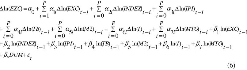
t DUM t MTO t I t M t TB t IPI t INDEX t EXC i t MTO P i i i t I P i i i t M P i i i t TB P i i i t IPI P i i i t INDEX P i i i t EXC P i i EXC ε β β β β β β β β α α α α α α α α + + − + − + − + − + − + − + − + − = ∆ + − = ∆ + − = ∆ + − = ∆ + − = ∆ + − = ∆ + − = ∆ + = ∆ 8 1 ) ln( 7 1 ) ln( 6 1 ) 2 ln( 5 1 ) ln( 4 1 ) ln( 3 1 ) ln( 2 1 ) ln( 1 ) ln( 0 7 ) ln( 0 6 ) 2 ln( 0 5 ) ln( 0 4 ) ln( 0 3 ) ln( 0 2 ) ln( 1 1 0 ) ln( (6)
where α0 is constant. EXC is the exchange rate, INDEX is the stock market index,
IPI is industrial production index, TB is the trade balance, M2 is money supply, I is
the interest rate, MTO is the degree of trade openness of Malaysia and DUM is the
dummy variable that represents the occurance of the financial crisis.
[image:13.612.135.538.146.261.2]4.RESULTS DISCUSSIONS
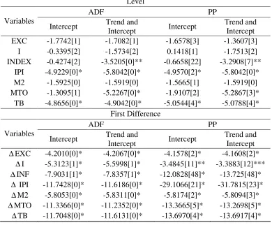
Table 1 shows that IPI, MTO, INDEX and TB are I(0), while the rest of the variables
are I(1). Because of the mixture of I(0) and I(1) data in the model and the dependent
variable, which is nominal RM/USD is I(1), the estimation of RM/USD is conducted
by applying the ARDL test.
Table 1
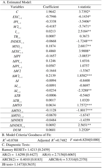
Table 2 demonstrates the most parsimonious ARDL model generated from the
Hendry’ general to specific method. This model has the lowest AIC value and passed
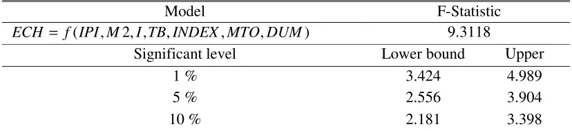
all the diagnostic test. The Wald test of ARDL rejects the null hypothesis if the
13 3, the F-statistic value is 9.5423, well above the critical value at all significant level.
Hence, the results indicate the presence of long-run relationship.
Table 2
Table 3
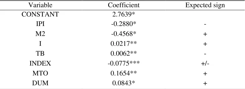
Thus, the long-run elasticities are generated and the coefficient of all variables are
summarized and reported in the Table 4. All the variables are statistically significant
and carried the expected signs, except for money supply and trade balance. The
results suggest that the increase in Malaysian degree of trade openness and interest
rate can lead to depreciation in Malaysian Ringgit. Besides, the rise of the income
level in Malaysia will lead to the appreciation of domestic currency which are in line
with the theory. As per expected, the occurrence of financial crisis in 2008 brought
down the value of RM against USD.
It is worth to discuss about the sign of coefficient of stock market index. As per
discussed in the section of theoretical framework, the impact of the rise in the
exchange rates depend on the relative strength of wealth effect and substitution effect.
The result in Table 4 indicates that there is negative relationship between exchange
rate and stock price. This means, the wealth effect excess the substitution effect in
Malaysia. This is actually in line with the findings of Baharumshah, Masih & Azali
(2002) and Broome and Morley (2003).
14 Although money supply did not carried the expected sign, the negative coefficient
sign of money supply can be explained by neo-classical growth theory and Tobin
effect. Both theory proposes that the increasing money supply will drive up the
inflation rate. This causes a rational individual to switch the asset allocation from
money in hand into another form of asset, like bond and lead to decrease in the
interest rate. Thus, the capital accumulation will increase and cause the increase in
output. As the increasing in output will cause the decrease in the domestic price level
and thus the appreciation in the exchange rate3. The Parikh (1992) also find out the
same conclusion. Nevertheless, this outcome contradicts with Baharumshah, Masih
& Azali (2002) findings. This may due to difference proxy for the money supply
where they adopted the M1 as the proxy for money supply.
Meanwhile, the positive coefficient of trade balance differential might be explained
by the reason that even though Malaysian trade balance increases in relative to the
US trade balance, the international capital might not flow into Malaysia as there are
many more options for the investor to invest in. At the same time, the increasing
trade balance in Malaysia could induce the Malaysian authority to depreciate the
Malaysian Ringgit intentionally in the effort to maintain the trade balance
performance.
In short, the long-run relationship can be expressed in the following equation
ECH = 2.7639 - 0.2880IPI - 0.4568M2 + 0.0217I + 0.0063TB + 0.1654MTO - 0.0775INDEX + 0.0843DUM (7)
3
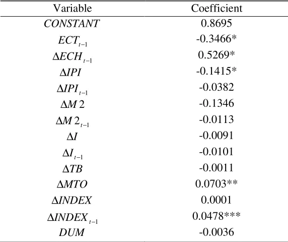
15 In the short-run, the error correction term is significant with negative coefficient.
This indicates that any disequilibrium that deviate the exchange rate from its
long-run equation in the short-long-run will be corrected. Only changes in ECH, IPI, MTO and
INDEX can change the exchange rate in the short-run as per shown in Table 5. The
magnitudes of the impact of the changes of statistically significant variables are also
much lower than the magnitudes in the long-run. The INDEX has the opposite sign,
means that in the short run, people tends to invest in the stock market and reduce the
money demand, hence depreciates Malaysian Ringgit.
Table 5
5. SUMMARY, CONCLUSIONS AND POLICY RECOMMENDATIONS
5.1 Summary and Conclusions
Exchange rate stability has become the external targets of Malaysia, aside of the
internal target, which is the price stability. Since Malaysia is a small and open
economy which involved heavily in international trade and the economic theory
suggested by Dornbush (1974) highlighted that the elimination of tariff (greater trade
openness) will cause currency depreciation by reducing the price of exportable goods
and increase the price of importable goods, this study attempts to examine the impact
of trade openness on Malaysian exchange rate. Variables from monetary and
portfolio balance approach are included beside trade openness in the model of
exchange rate.
The findings from ARDL estimation show that in the long-run, all independent
16 supply and trade balance. As predicted by the theory, the rise of the income level and
stock market index in Malaysia will lead to the appreciation of domestic currency,
increase in trade openness and interest rate lead to depreciation of Malaysian Ringgit.
The negative coefficient of the stock market index also indicates that the wealth
effect surpass the substitution effect when the equity price increase. However, not all
the independent variables behave according to the theories. In this study, rise in
money supply differential caused RM to appreciate. Neo classical growth theory and
Tobin effect have been offered as the explanation of the appreciation of RM/USD
following increase in the domestic money supply. On the other hand, increase in
trade balance caused the depreciation of RM due to country has involved in the
currency manipulation to maintain their surplus position on the trade balance. In the
short-run, only Malaysia trade openness, stock market differential, industrial
production index (income) differential and RM/USD itself influence the RM/USD.
5.2 Policy Recommendations
Several recommendations are suggested from the outcomes of the study. Since the
results showed that open economic policy can cause the depreciation of RM/USD,
Malaysia should maintain the policy of open economic. Open economic policy has
successfully raised Malaysia position in the international trade. Currency
depreciation increases the competitiveness of Malaysia exporters and encourage
domestic producer and importer to venture into cost effective production mode to
save costs. Although increase in Malaysia trade balance tends to depreciate RM, but
the control of Malaysia on the trade balance is limited as the increase in trade balance
depend on the purchasing power of the foreign importers and the competitiveness
17 Results also indicate that increment in domestic interest rate will dampen our
exchange rate and increase in money supply, on the other hand, strength the RM.
This findings shows that monetary policy is a useful tool in controlling the
movement of Malaysian Ringgit. While increase in the interest rate could cause
further capital inflows that might weaken the soundness of Malaysian Financial
market, Malaysian government has done well in sterilizing the excess monetary base.
In order to strength RM, government share increase the productivity in the long run.
High productivity can increase the level of income in Malaysia as Malaysian
products and services become more competitive internationally. This can be done by
encouraging more high technology production and increase the quality of human
capital.
Since the bull stock market strengthen RM, government should encourage more
listing of local and foreign companies with good fundamental in domestic bourse. To
do this, more incentives to companies to list their entities in bourse and better
surveillance on stock exchange trading and operation can stimulate positive
development in the stock market. In the short-run, booming stock market can
depreciate the Malaysian Ringgit. Ensuring the transparent and complete
dissemination of market information and good governance in government and
companies can create vivid stock market and let the value of companies with good
foundation to be fully realized and increase the stock market return. However, the
18
5.3 Limitations and Suggestions
There are several limitations and suggestions that can be issued in this section.
Others measurements of trade openness can be used to replace the measurements
applied in this research. Besides, there could be exist non-linearity among the
dependent variable and independent variables4. Future research can consider adding
in the financial linkage between Malaysia and US in the estimation. Finally, the
rising of China as the ‘world factory’ and increasing trade volume with China makes
it desirable for the future researcher to focus about the determinants of RM/China
Renminbi.
4
19
REFERENCES
Abdalla, I.S.A. and Murinde, V. (1997). Exchange rate and stock price interaction in emerging financial markets: evidence on India, Korea, Pakistan and the Philippines. Applied Financial Economics, 7, 25–35.
Aydemir, O. and Demirhan, E. (2009). The relationship between stock price and exchange rate evidence from Turkey. International Research Journal of Finance and Economics, 23, 207-215.
Azman-Saini, W.N.W., M.S. Habibullah and M. Azali (2003). Stock prices and exchange rate interactions in an emerging market, RISEC: International Review of Economics and Business, 50, 503-519.
Baharumshah, Z. A., Masih, M. M. A. and Azali, M. (2002). The stock market and the ringgit exchange rate: a note. Japan and the World Economy, 14,.471-486.
Baharumshah, Z. A, Mohd, S.H. and Ahn, S.K(2009). On the predictive power of monetary exchange rate model: the case of the Malaysian ringgit/US dollar rate. Applied Economics, 41, 1761-1770.
Bahmani-Oskooee, M. and Sohrabian, A. (1992). Stock prices and the effective exchange rate of the Dollar. Applied Economics, 24, 459-464.
Beckmann, J., Belke, A. and Kuhl, M. (2011). The dollar-euro exchange rate and macroeconomic fundamentals: a time-varying coefficient approach, Review of World Economics, 147, 11–40.
Branson, William H, H. Haltunen and Paul R. Masson (1977). Exchange rate in the short-run: The dollar-dentschemark rate. European Economic Review, 10, 303-324.
Broeck, D. M. and Slok, T. (2001). Interpreting real exchange rate movements in transition countries. Discussion Papers (No.7). Helsinki, Finland: Bank of Finland Institute for Economies in Transition.
Broome, S and Morley, B. (2003). Stock Prices and the Monetary Model of the Exchange Rate: An Empirical Investigation, Unpublished Manuscript. Department of Economics, National University of Ireland Maynooth. Retrieved from http://ideas.repec.org/p/may/mayecw/n1321103.html
Caldelon, B, Kool, C., Raabe, K. and Veen, V. T. (2007). Long-run real exchange rate determinants: Evidence from eight new EU member states, 1993-2003.
Journal of Comparative Economics, 35, 87-107.
Carrera, J. and Resout, R. (2008). Long run Determinants of Real Exchange Rates in Latin America. Working Papers (W.P.08-11). Ecully, France: GATE
Chinn, M. D. (2000a). Three measures of East Asian currency overvaluation.
20 Chinn. M. D. (2000b). Before the fall: were East Asian currencies overvalued?
Emerging Market Review,1, 101-126.
Diamandis, P. F., Georgoutos, D. A. and Kouretas, G. P. (1998). The monetary approach to the exchange rate: long-run relationships, identification and temporal stability, Journal of Macroeconomics,20, 441-466.
Doong, S.C., Yang, S.Y. and Alan Wang, T. (2005). The dynamic relationship and pricing of stocks and exchange rate: Empirical evidence from Asian emerging markets. Journal of America Academy of Business, Cambridge. 7, 118-123.
Dornbusrch, R. (1974). Tariffs and nontraded goods. Journal of International Economics,. 4, 177-185.
Economy of Malaysia. (n.d.) Retrieved January 07, 2010, from Wikipedia: http://en.wikipedia.org/wiki/Economy_of_Malaysia
Egert, B. (2005) Equilibrium exchange rates in South Eastern Europe, Russia, Ukraine and Turkey: Healthy or (Dutch) diseased? Economic Systems, 29, 205-241.
Egert, B. (2010) The Impact of monetary and mommodity fundamentals, macro news and central bank communication on the exchange rate: Evidence from South Africa. Open Economies Review, 21, 655–677.
Gandolfo, G, Martinengo, G. and Padoan, C. P. (1981). Qualitative Analysis and Econometric Estimation of Continuous Time Dynamic Models. Netherland: North-Holland.
Gokal, V. and Hanif, S. (2004). Relationship between Inflation and Economic Growth. (Working Paper 2004/04). Suva, Fiji: Economics Department, Reserve Bank of Fiji. Retrieved from http://www.reservebank.gov.fj/docs/2004_04_wp.pdf
Groen, J. J. J. (2000). The monetary exchange rate model as a long-run phenomenon.
Journal of International Economics, 52, 299-319.
Hooper, P. and Morton, J. (1982). Fluctuations in the dollar: A model of nominal and real exchange rate determination. Journal of International Money and Finance, 1, 39–56.
Husted, S. MacDonald, R. (1999). The Asian currency crash: were badly driven fundamentals to blame? Journal of Asian Economics,10, 537-550.
Ibrahim, H. M. (2000). Cointegration and Granger causality tests of stock price and exchange rate interactions in Malaysia. ASEAN Economic Bulletin, 17, 36-47.
Jeong, J.G. (2000). What Drives Exchange Rates?: The Case of The Yen/Dollar Rate.
21 Kouretas, G. P. (1997). Identifying linear restrictions on the monetary exchange rate model and the uncovered interest parity: cointegration evidence from the Canadian U.S. dollar. Canadian Journal of Economics,30, 875-890.
Lane, P.R. and Milesi-Ferretti, G.M. (2002). External wealth, the trade balance, and the real exchange rate, European Economic Review, 46, 1049 – 1071.
Lee, C., Azali, M. and Masih, A.M.M. (2009). Tests of the different variants of the monetary model in a developing economy: Malaysian experience in the pre- and post-crisis periods. Applied Economics, 41, 1893-1902.
Lee, C., Azali, M. and Matthews, K.G. (2007). The monetary approach to exchange rate determination for Malaysia. Applied Financial Economics Letters, 3, 91-94.
Li, X. M. (2004). Trade liberalization and real exchange rate movement. IMF Staff Papers, 51, 553-584.
Liew, K.S, Baharumshah, A.Z., Habibullah, M.S. and Midi, H. (2011). ASEAN-5 exchange rate determination in the presence of nonlinearity. Journal of International Economic Review, 4, 1-11.
Liew, K.S. (2009). Linear and nonlinear monetary approaches to the exchange rate of the Philippines peso-Japanese yen. Economics Bulletin, 29, 1331 - 1440.
MacDonald, R. and Taylor, M. P. (1991). The monetary approach to the exchange rate: long-run relationships and coefficient restrictions, Economics Letters,37, 179-185.
MacDonald, R. and Taylor, M. P. (1993). The monetary approach to the exchange rate: rational expectations, long-run equilibrium, and forecasting. IMF Staff Papers,40, 89-107.
MacDonald, R. and Taylor, M. P. (1994a). The monetary model of the exchange rate: long-run relationships, short-run dynamics and how to beat a random walk,
Journal of International Money and Finance,13, 276-290.
MacDonald, R. and Taylor, M. P. (1994b). Re-examing the monetary approach to the exchange rate: the Dollar-Franc, 1976-90, Applied Financial Economics, 4, 423-429.
MacKinnon, G. J. (1996). Numerical distribution function for unit root and cointegration tests. Journal of Applied Econometrics, 11, 601-618.
Melecky, M. and Komarek, L. (2007). The behavioral equilibrium exchange rate of the Czech Koruna. Transition Studies Review, 14, 105-121.
22 Pan, M. S., Robert Fok, C. W. and Angela Liu, Y. (2007). Dynamic linkage between exchange rates and stock prices: Evidence from East Asian markets.
International Review of Economics and Finance, 16, 503-520.
Parikh, A. (1992). An econometric study on the Yen-Pound exchange rate.
International Review of Economics and Finance, 1, 219-234.
Pesaran, M.H., Shin, Y.C. and Smith, J. R. (2001). Bound testing approaches to the analysis of level relationship. Journal of Applied Econometrics, 16, 289-326.
Rahman, L. M. and Uddin, J. (2009). Dynamic relationship between stock prices and exchange rates: Evidence from three South Asian countries. International Business Research, 2, 167-174.
Rapach, D. E. and Wohar, M. E. (2002). Testing the monetary model of exchange rate determination: new evidence from a century of data. Journal of International Economics, 58, 359-385.
Sarantis, N. (1987). A dynamic asset market model for the exchange rate of the pound sterling. Weltwirtschaftliches Archiv, 123, 24–38.
Sidek, N.Z and Yusoff, M. (2009). An empirical analysis of Malaysian Ringgit Equilibrium exchange rate and misalignment. Global Economy & Finance Journal, 2, 104-126.
Smith, C. (1992a). Stock markets and the exchange rate: a multicountry approach.
Journal of Macroeconomics, 14, 607–629.
Smith, C. (1992b). Equities and the UK exchange rate. Applied Economics, 24, 327– 335.
Solnik, B. (1987). Using financial price to test exchange rate models: A note. Journal of Finance, 42, 114–119.
Tawadros, G. B. (2001). The predictive power of the monetary model of exchange rate determination. Applied Financial Economics, 11, 279-286.
23 Table 1. Stationary tests
Level
ADF PP
Variables
Intercept Trend and
Intercept Intercept
Trend and Intercept EXC -1.7742[1] -1.7082[1] -1.6578[3] -1.3607[3]
I -0.3395[2] -1.5734[2] 0.1418[1] -1.7513[2] INDEX -0.4274[2] -3.5205[0]** -0.6658[22] -3.2908[7]**
IPI -4.9229[0]* -5.8042[0]* -4.9570[2]* -5.8042[0]* M2 -1.5925[0] -1.5919[0] -1.5665[1] -1.5919[0] MTO -1.3095[1] -5.2267[0]* -1.9107[2] -5.2867[3]*
TB -4.8656[0]* -4.9042[0]* -5.0544[4]* -5.0788[4]* First Difference
ADF PP
Variables
Intercept Trend and
Intercept Intercept
Trend and Intercept
∆EXC -4.2010[0]* -4.2067[0]* -4.1578[2]* -4.1608[2]*
∆I -5.3123[1]* -5.5998[1]* -3.4845[11]** -3.3883[12]***
∆INF -7.9031[1]* -7.8357[1]* -12.0828[48]* -13.725[48]*
∆ IPI -11.7428[0]* -11.6186[0]* -29.1066[21]* -31.7815[23]*
∆M2 -5.8053[0]* -5.8311[0]* -5.8174[2]* -5.8094[3]*
∆MTO -11.3366[0]* -11.2352[0]* -13.3665[5]* -13.2698[5]*
∆TB -11.7048[0]* -11.6131[0]* -13.6970[4]* -13.6917[4]*
24 Table 2. Estimated ARDL model for RM/USD
A. Estimated Model:
Variables Coefficient t-statistic
C 1.9642 3.7392*
1
−
t
EXC -0.7946 -6.1434*
1
−
t
IPI -0.3338 -3.5406*
1
2t−
M -0.4187 -5.7471*
1
−
t
I 0.0213 2.5184**
1
−
t
TB 0.0007 0.3673
1
−
t
INDEX -0.0668 -1.7248***
1
−
t
MTO 0.1874 2.6817**
1
−
∆EXCt 0.4860 3.9008*
IPI
∆ -0.1657 -3.0853*
1
−
∆IPIt 0.1246 1.6516
2
−
∆IPIt 0.0587 1.0757
2
M
∆ -0.1644 -1.5367
1
2−
∆M t 0.2139 1.8582***
I
∆ -0.0094 -0.8400
1
−
∆It -0.0091 -0.8697
2
−
∆It -0.0234 -2.3288**
TB
∆ -0.0006 -0.5465
1
−
∆TBt 0.0017 1.0320
MTO
∆ 0.0634 1.7572***
1
−
∆MTOt -0.1128 -1.8017***
2
−
∆MTOt -0.0670 -1.6747
INDEX
∆ -0.0484 -1.4359
1
−
∆INDEXt 0.0692 2.5651**
DUM 0.0601 3.2520*
B. Model Criteria/ Goodness of Fit:
2
R =0.8768 Adjusted R2=0.7482 Fstat=6.8204[0.000]
C. Diagnostic Tests:
Ramsey RESET= 1.4213 [0.2459]
AR(2) = 1.6298 [0.4427] AR(4) = 2.7156[0.6065]
ARCH(2) = 0.4010 [0.8183] ARCH(4) = 5.5316[0.2370] JB test= 1.1473[0.5635]
25 Table 3. Bound test for exchange rate model cointegration analysis
Model F-Statistic
) , , ,
, , 2 ,
(IPI M I TB INDEX MTO DUM f
ECH = 9.3118
Significant level Lower bound Upper
1 % 3.424 4.989
5 % 2.556 3.904
10 % 2.181 3.398
26 Table 4. The long-run elasticities of exchange rate model for RM/USD
Variable Coefficient Expected sign CONSTANT 2.7639*
IPI -0.2880* -
M2 -0.4568* +
I 0.0217** +
TB 0.0062** -
INDEX -0.0775*** +/-
MTO 0.1654** +
DUM 0.0843* +
27 Table 5. The short-run elasticities of exchange rate model for RM/USD
Variable Coefficient
CONSTANT 0.8695
1
−
t
ECT -0.3466*
1
−
∆ECHt 0.5269*
IPI
∆ -0.1415*
1
−
∆IPIt -0.0382
2
M
∆ -0.1346
1
2−
∆M t -0.0113
I
∆ -0.0091
1
−
∆It -0.0101
TB
∆ -0.0011
MTO
∆ 0.0703**
INDEX
∆ 0.0001
1
−
∆INDEXt 0.0478***
DUM -0.0036