What Is the Difference between Gamma and Gaussian Distributions?

(1)

What Is the Difference between Gamma and

Gaussian Distributions?

Xiao-Li Hu

School of Electrical Engineering and Computer Science, University of Newcastle, Newcastle, Australia Email: xiaoli.hu@newcsatle.edu.au, xlhu@amss.ac.cn

Received November 19, 2012; revised December 25, 2012; accepted January 3, 2013

ABSTRACT

An inequality describing the difference between Gamma and Gaussian distributions is derived. The asymptotic bound is much better than by existing uniform bound from Berry-Esseen inequality.

Keywords: Gamma Distribution; Gaussian Distribution; Berry-Esseen Inequality; Characteristic Function

1. Introduction

1.1. Problem

We first introduce some notations. Denote Gamma distribution function as

 

_{ }

1

0 1

, e d

x

k t

k x t t

k

 

 





(1)

for and , where is the Gamma function, i.e.,

0

k x0 

 

k

 

1

0

e d .

k t

  

 

_

t 0

Assume 

 

k x,  for x0. The density of chi-

square distributed random variable n with n degrees of freedom is

 

1

2 2

2 1

e , for 0,

, 2

2

0, otherwise.

n x

n x x

n f_ x n

 



 

    _{ }   



It is well-known that the random variable n can be in- terpreted by 2

1 n

n k

k

 





with independent and iden- n tically distributed (i.i.d.) random variables _k 

 

0,1 ,

where

1, 2, ,

k  n 



0,1



denotes the standard Gaussian distribution. The mean and variance of n is respectively





2

, 2

n n

E n E  n  n.

Then, by simple change of variable we find

,

2 2 2

2

n n n n n

P x x

n

   

 _ _{ } _ 

  _

   

On the other side, by the Berry-Esseen inequality to







2 ₁ _{2 ,} _{1, ,}



k k

    n , it is easy to find a bound 0

C such that

 

,

2

n n C

P x x

n n

 

 

   

 

  (3)

where 

 

x is the standard Gaussian distribution func-

tion, i.e.,

 

2

1 _e _{d .}

2π

x x

x  x



 

_

(4) Then, by Equations (2) and (3) it follows

 

, ,

2 2 2

n n n C

x x

n

 

_  _  

  (5)

which describes the distance between Gamma and Gau- ssian distributions. The purpose of this paper is to derive asymptotic sharper bound in Equation (5), which much improves the constant by directly using Berry-Esseen inequality. The main framework of analysis is based on Gil-Pelaez formula (essentially equivalent to Levy inversion formula), which represents distribution function of a random variable by its characteristic function.

C C

The main result of this paper is as following.

Theorem 1.1 A relation of the Gamma distribution (1)

and Gaussian distribution (4) is given by

 

sup , ,

2 2 2

x

C n

n n n

x x

n

 

_  _  

  (6)

where

 

1

 

1

, 3 π

C n  C n

.

(2)

 





2 0

1

2

1 0

2 ₆

0 ₀

1 3

3 π 2 2π

e 2

π π e π

n

C n

n n

n n n

n

n n n





 



  

with 1

2 n n  and

1 6 3 0

n n

 

 for any 0,1 2 _{ } _

 .

Clearly, as . Thus, the asymp- totical bound is 1

 

0

C n  n 

 

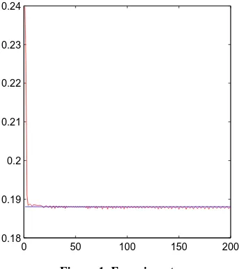
1 0.1881

3 π

C n   

as . To check the tightness of the limit value of , we plot in Figure 1 the multiplication

n 

 

C n

 

2 2

sup ,

2 2 2

n n

x

n n n

n x

  

 

 _  _ 

  x

for n1, 2, , 200 , where the straight line is the limit value 1

3 π. From this experiment it seems that

1 3 π

is the best constant. The tendency of the theoretical formula C n

 

is plotted for n

 

1,10 10 14 in Figure 2, which also shows the tendency to the limit value

1

3 π . The slow trend is due to that some upper bounds

formulated over interval



n n₀, ₁



have been weakly es-

timated, e.g., the third and fourth terms of C n₁

 

. 1.2. Comparison to the Bound Derived by

Berry-Esseen Inequality

Let be a sequence of independent identi- cally distributed random variables with EX1 = 0



X X1, 2,



2

1 1

EX 

0 50 100 150 200

[image:2.595.337.507.82.273.2]

0.18 0.19 0.2 0.21 0.22 0.23 0.24

Figure 1. Experiment.

2 4 6 8 10

x 1014 0.188

0.1881 0.1882 0.1883 0.1884 0.1885 0.1886

Figure 2. Trend of C n .

and finite third absolute moment  3 E X13 . De- note

 

1 n _.

n

X X

F x P x

n

 

 

 _  _

 



By classic Berry-Esseen inequality, there exists a finite positive number C0 such that



_,



_sup

 

0 3_.

n n

x

C

d F F x x

n 

     (7) The best upper bound ₀ is found in [1] in 2009. The bound is improved in [2] at some angle in a slight different form as

0.4785

C 



_,



1

n

C d F

n

  (8) with













1 min 0.33477 3 0.429 ,0.3041 1 .

C    3

The inequality (8) will be sharper than Equation (7) for 3 1.93

  .

Now let us derive the constant C in (5) by applying Berry-Esseen inequality to





2 ₁



_{2 ,} _{1, 2,}



k k

    . It is difficult to calculate the exact value of third absolute moment of the random variable



2



1 1

  2. Thus, it is approximated as

3 2 1 3

1

3.0731 2 2

E

    

by using Matlab to integrate over interval



0,100



di- vided equivalently 100,000 subinterval for its half value.

By Equation (7) with C00.4785 we have 0 3 1.4705

C  

[image:2.595.87.259.532.726.2]

(3)

1 1.1724 .

C  

Hence, the best constant in Equation (5) by applying Berry-Esseen inequality is . Obviously, the limit bound

C

1.1724

 

1

lim 0.1881

3 π

nC n   

found in this paper for chi-square distribution is much better.

The technical reason is that the Berry-Esseen inequality deals with general i.i.d. random sequences with- out exact information of the distribution.

2. Proof of Main Result

Before to prove the main result, we first list a few lemmas and introduce some facts of characteristic function theory.

2.1. Some Lemmas

Lemma 2.1 For a complex number z satisfying z 1,





ez 1 1

z z

   .

Proof First show that

2 ez 1

z z

   .

By Taylor’s expansion and noting z 1, we have

2 2

2

0

e 1

! !

.

2 2

k k

z

k k

k

z z

z

k k

z z

z

 

 





   

     

 



Together with

ez 1 ez 1

z z

     ,

the assertion follows.

Lemma 2.2 For a real number x satisfying x < 1,





1i

 

3 i

1 i exp 1

2

x x ,

x  R x 

  _   _

 

where is the imaginary unit and i

 

2 4 6

3

3 5 7

i .

4 6 8

x x x

R x

x x x

 

 _    _

 

 

 _    _

 



Clearly,

 

2 3

3

1 1 _.

3 4

R x  x  x

Proof. By Taylor expansion for complex function, for

< 1

x we have





     

   

 

2 3 4

2 3

3

i i i

1 1

ln 1 i i

i i 2 3 4

i i

i 1

2 3 4

i

1 ,

2

x x x

x x

x

R x

 

 

     

 

 

    

  



where R3

 

x is shown above. By further noting the two

alternating real series above, it follows the upper bound. We cite below a well-known inequality [3] as a lemma.

Lemma 2.3 The tail probability of the standard nor- mal distribution satisfies

2 2

1 1

2 2

2

1 _e 1 _e _d 1 1

1 2π 2π 2π

2

1 2 e

x t x

x

t x x



 

   







for x0.

2.2. Characteristic Function

Let us recall, see e.g., [4], the definition and some basic facts of characteristic function (CF), which provides another way to describe the distribution function of a random variable. The characteristic function of a random variable X is defined by

 

_{e ,}itX

X t E

 

where is the imaginary unit, and is the argument of the function. Clearly, the CF for random variable

i

X

tR

Y a b with real numbers a and b is

 

_{e .}ibt

Y t X at

 

Another basic quality is

 

  

Z t X t Y

   t



for Z XY with X and Y independent to each

other.

It is well-known that the CF of standard Gaussian

 

0,1

 is

 

_t _e 12t2

   (9) and the CF of chi-square distributed variable n is

  

1 2i



2.

n

t t



 _{ } 

Thus, the CF for

2

n n

S n

 

 is

 

₁ 2i 2_e 2i

n n t

S

t t

n 

 

  _  _

  . (10)

(4)

of density function. Therefore, distribution function can be expressed by CF directly, e.g., Levy inversion formula. We use another slightly simpler formula. For a univariate random variable X, if x is a continuity point of its distribution FX, then

 

i

 

i

 

0

e e

1

d ,

2 2πi

tx tx

X X

X

t t

F x t

t

  

 _{ }

 

_

(11)

which is called Gil-Pelaez formula, see, e.g., page 168 of [4].

2.3. Proof of Main Result

We are now in a position to prove the main result. Proof of Theorem 1.1 First analyze CF of

2

n n

S n

 



given by Equation (10). Denote x 2t n

  . For x < 1,

i.e.,

2 n

t  , by Lemma 2.2,

 

i i 2i 2

2

3 2i

1 e

exp ,

2 n n t

n t t

S

t t

n

t R t



 _ 

 

 _ _

 

 

 _  _

 

(12)

where

 

3 3

2 4

3 5

i 2 i

3 5 2

. 4 6 2

n t

R t R x

n t x x

nt x x



 

  _   _

 

 

 _   _

 



Clearly,

 

2 3

3

3 ₄

1 1

3 4

2 2

. 2 3

n t

R t x x

t t

n n

 

 _  _

 

 

To make sure R t3

 

n



 for some 



0,0.5



, denote

1 6 3 0

n n

 

 . Then, it is easy to see that

 

3 4

3

2 2 3

2 1 1 1 ₁

3 2

t t

R t

n n

n n

 

 

_  _  

 

(13)

for t n0 . Hence, by Equations (12) and (13) and

Lemma 2.1,

   

 



 







 

2

2 2

3 2

2 2

3 3 3

e e 1

e 1 e 1

t R t S

t t

R t R t n R t

  

  _

  

   

(14)

for t n0.

Now let us consider the difference between S

 

t

and 

 

t , i.e., the CF (9) of Gaussian distribution, over the interval



0,n0



. By Equation (14)

   





   

 

0

2

0 0

2 2

0 0

i

0

3 2

0 0

3

2 2 2

0 0

e

d 2πi

1

d e

2π 2π

1 2 _{e d} 1 _{e d .}

2π 3 2

tx n

S

n n t

S

n t n t

t t

R t

t t n

t t

n

t t t t

n n



 



 _

 _ _



 

  d

 

 _ _

 

 

 



Note that

2 2

3

2 2 2

0 0

2π 3 2π

e d , e d ,

2 2

t t

t t t t

 _  _

 



it follows

   





0 i

0 e

d 2πi

1 1 3 _.

6 π 4 2π tx

n

S t t

t t

n

n n



 



 

  

 _  _

 



(15)

Similarly,

   





0 i

0 e

d 2πi

1 1 3

. 6 π 4 2π tx

n

S t t

t t

n

n n



 



  

  

 _  _

 



(16)

Below let us analyze the residual integrals over the interval



n₀,



. By Lemma 2.3,

 

2

0 0

2 2

0

i ₂

2 2

2 0 0

e e

d d

2πi 2π

1 e _d e _.

2π

2π 2π

t tx

n n

n t

n

t

t t

t n n

 



 

 





 



(17)

Similarly,

 

02

0

i ₂

2 0

e _d e

2πi 2π

n tx

n

t t

t n

 

 _



(5)

over for . We divide it into two subin- tervals as following:



0



,

n  _S

 

t

 

2 0 0

i

1 0

6 0

e _d 1 _.

2πi ₂_π _e π

tx S

n n

t n n

t

t _n n





 _

 



(21)

 





0 0 0

1

0 1

2

2 4

i

2 ₄

1 2

2i 2

1 d 1 d

e

d

2πi 2π 2π

2

1 d

, 2π

n n

tx S

n n n

n

n n

t t

t n n

t

t t

t t n

t

I I

t 

 



  





 

 _  _

 

 

      

  



 



Similarly,

 

2 6 0 0

i

1 0

0

e 1

d .

2πi ₂_π _en π

tx S

n

t n n

t

t _n n



 _ _

 



(22)

By Equation (15), Equation (17), Equation (21) and Equation (16), Equation (18), Equation (22)

   

 

i i

0

i

0

i

0

e e

d 2πi

e

d 2πi

e

d ,

2πi

tx tx

S S

tx S

t t t t

t t

t t C n

t

t n

   

 

 



 

    

   

   

  

 

 





 

 

 



where 1

2 n

n  .

Observe that

2 ₄

1 ₁ 2

n

t

t n



    

  decreases on interval



n n0, 1



and

1 1

1 e

x



 _  _

 

  for x1, we have

where

   0

0 2 0

1 0 1

2 4 0 0

1 0 1 0

1 0

2 ₂ 0 0

2π

2 1

, e 2

1

n

n n

I

n n

n

n n n n

n n

 

 

  

 

 

 

      

 

 

      

 





2 0

2 6 0

1

2

1 0 2

0 ₀

1

,

3 π

1 3

3 π 2 2π

e 2

.

π π en π

n

C n C n

C n

n n

n n n

n

n n n





 



  

where

 









2 2

0 0

0 2

0

4 _.

2 2 6

2 2 1

2 n

n n n n n

n

n n n n n

n

    

 



2 0

n

In view of Formula (11) , the formula to be proved follows directly.

REFERENCES

[1] I. S. Tyurin, “On the Accuracy of the Gaussian Approxi- mation,” Doklady Mathematics, Vol. 80, No. 3, 2009, pp.

840-843. doi:10.1134/S1064562409060155 The fact 2 is used in above formula. Thus,

0

n 

2 0

1 0

1 ₆

0 , 2π en

n n

I n



 (19)

For the other interval



n1,



, we proceed as

1 1

1

2

2 4 2 4

1

4 4

2

d d

2π

2 2

1

2 2

d

2 2 2

n n

n

t t

I

t t

n n

n n n

t t

n n

4 .

n

   

 

    

              _{ } _{ }  _{ } 

     



[2] V. Koroleva and I. Shevtsova, “An Improvement of the Berry-Essen in Equality with Application to Possion and Mixed Poison Random Sums,” Scandinavian Actuarial Journal, Vol. 2012, No. 2, 2012, pp. 81-105.

doi:10.1080/03461238.2010.485370

 

[3] R. D. Gordon, “Values of Mills’ Ratio of Area to Bound- ing Ordinate and of the Normal Probability Integral for Large Values of the Argument,” The Annals of Mathe- matical Statistics, Vol. 12, No. 3, 1941, pp. 364-366.

doi:10.1214/aoms/1177731721 (20)

[4] K. L. Chung, “A Course in Probability Theory,” 3rd Edi- tion, Probability and Mathematical Statistics, Academic,