Human activity recognition making use of long short term memory techniques

memory techniques

WAINWRIGHT, Richard and SHENFIELD, Alex <http://orcid.org/0000-0002-2931-8077>

Available from Sheffield Hallam University Research Archive (SHURA) at:

http://shura.shu.ac.uk/24115/

This document is the author deposited version. You are advised to consult the publisher's version if you wish to cite from it.

Published version

WAINWRIGHT, Richard and SHENFIELD, Alex (2019). Human activity recognition making use of long short-term memory techniques. Athens Journal of Sciences, 6 (1), 19-34.

Copyright and re-use policy

Human Activity Recognition Making Use of Long

Short-Term Memory Techniques

By Richard Wainwright

& Alex Shenfield

The optimisation and validation of a classifiers performance when applied to real world problems is not always effectively shown. In much of the literature describing the application of artificial neural network architectures to Human Activity Recognition (HAR) problems, postural transitions are grouped together and treated as a singular class. This paper proposes, investigates and validates the development of an optimised artificial neural network based on Long-Short Term Memory techniques (LSTM), with repeated cross validation used to validate the performance of the classifier. The results of the optimised LSTM classifier are comparable or better to that of previous research making use of the same dataset, achieving 95% accuracy under repeated 10-fold cross validation using grouped postural transitions. The work in this paper also achieves 94% accuracy under repeated 10-fold cross validation whilst treating each common postural transition as a separate class (and thus providing more context to each activity).

Keywords: LSTM, Neural Networks, Postural, Recurrent Neural Network; Human Activities.

Introduction

Human activity recognition (HAR) is an old concept. Similar to ubiquitous computing, a sensor is used to collect data from the user to try and assist a user with a given task. HAR has a vast number of applications, including in the military domain, medical facilities, fitness tracking and in regular daily life. Nike have produced running shoes that contain integrated motion sensors to provide feedback and running statistics for athletes (Johnson 2018).1 Similarly, Apple’s latest watch OS update contains automatic activity/fitness detection to alert a user on their watch that they are working out and should begin to track this information (Hardwick 2018).

It is apparent that HAR is becoming more common in all aspects of daily life and therefore, this topic has become very attractive to researchers. Ongoing work means that basic activities including sitting and walking can be monitored and tracked reliably with a high level of accuracy if the user wears a high number of sensors nodes - unfortunately, it is not realistic to wear a large number of sensors. The introduction and popularity of the smartphone has helped to push research in this field, as these devices are usually equipped with both Gyroscopes and accelerometers; with some high-end devices providing 3 axial velocities from the accelerometer. People carry these devices with them all the time, so it provides an

*

Researcher, Sheffield Hallam University, Sheffield, UK.

obvious non-intrusive way of monitoring activities. Moreover, these devices are generally carried all day, so data can be collected anywhere. This allows us to obtain realistic data from real life situations.

This paper outlines an effective approach of detecting human activities making use of Long-Short Term Memory techniques with the novel aspect of additionally classifying postural transitions. Results presented show that this novel classification method is extremely effective as it provides high accuracy detection with a small number of false positives. 10-Fold repeated cross validation is introduced to validate the results obtained from the model.

The rest of the paper is organised as follows: The next section provides a brief background to existing HAR techniques within the smartphone/smart watch industry and introduces Long-Short-Term Memory recurrent neural network techniques. Section “Human Activity Recognition on Given Dataset”outlines the model setup and describes what validation methods were used and how they were applied to the proposed model. Section “Results” then describes the major milestones of the research completed and some potential developments for further work.

Background and Previous Work

Machine Learning Methods / Related Works

Machine learning techniques have been used for automatic classification of HAR throughout the literature. These ML techniques have been supervised, semi-supervised and unsemi-supervised with all different methods proposed. Standard models such as Frequentist and Bayesian models (for example, binary decision tree and threshold-based classifiers) have been implemented (Ermes et al. 2008, Coley et al. 2005). In addition, geometric models were introduced to detect HAR with papers describing K-Nearest Neighbours, Artificial Neural Networks and also Support Vector Machines (Maurer et al. 2006, Khan et al. 2010). Liu et al. (2016) made use of single frame images from Microsoft Kinects and RNN LSTM classifiers to correctly identify the activities in the images. The results obtained 95% peak accuracy when making gate modifications to the LSTM.

Currently, no obvious model or classifier is the most appropriate for HAR as all the different techniques have established performances that are comparable. In ML, the most effective classification method is generally application specific with additional considerations including computing power, energy consumption and memory requirements all are considered trade-offs for producing a reliable model.

Evaluation Metrics and Performance

types of errors made by the systems (false positives and true negatives) and correctly predicted results. Furthermore, the matrix allows the extrapolation of additional information including model accuracy, precision and F1-score. Confusion matrices, overall confusion matrix accuracy, best loss and best accuracy per fold will described and compared in this paper, they can be reviewed in the results section.

Long Short-Term Memory

Hochreiter and Schmidhuber (1996) proposed Long Shot Term Memory (LSTM) Units in the mid-90s as an alternative method of recurrent neural networks in order to combat the vanishing gradient problem

Unlike other networks, LSTMs preserve and maintain the errors so that they can be easily backpropagated through layers, which also make LSTMs useful for time series problems as this error can also be backpropagated through time. Preserving the error allows the recurrent network to continue to learn and train the model over a vast number of time steps. This solution opens a channel that allows causes and effects to be linked therefore removing the error at the source.

Analog gates are used in LSTMS where information can be stored, written to or read from – similarly to data stored within a computer. This gated cell contains information outside the regular flow of the recurrent neural network (RNN). The use of anlaog gates are implemented with element wise multiplication by varying functions such as sigmoids which are always in the range of 0-1. The implementation of analog over digital functions means that they are easily differentiated, therefore, making them suitable for backpropagation.

Each gate acts on the information/signals once they receive them, information can be blocked or passed on based on its strength and import. These signals are also filtered with each gates weight. These weights behave similarly to normal NN input and hidden states as they are adjusted throughout the RNN learning process. The cells learn when to permit data to: enter, be deleted or leave through the iterative processes found from backpropagating the errors, adjusting the weights and making informed guesses.

Architecture of LSTMs

Figure 1. LSTM Architecture Overview

Forget Gate

A forget gate is designed for eradicating information from the current cell state. The LSTM performance is optimized by the removal of any unnecessary information that is no longer needed by the LSTM to understand things or to remove any information that isn’t important anymore. The forget gate removes this information by the multiplication of a filter. A forget gate will take in two different inputs:

(1)

(2)

Equation (1) is the notation used to describe the hidden state from the previous cell whereas (2) is the input at that given time step. The two inputs are multiplied by the weight matrices at those times with an additional bias added. The resulting value then has a sigmoid function applied to it. Subsequently a vector with values from 0 to 1 is produced. The sigmoid function is responsible for telling the forget gate whether to discard or maintain the values. A resultant ‘0’ means that the values will be forgotten along with the information it contains. Alternatively, a ‘1’ means that the forget gate should retain that entire piece of information. The cell state and the vector output of the sigmoid are multiplied together.

Input Gate

The input gate is used to make sure that the all of information that is added to the cell stated is important and not redundant. The input gate can be described in a three-step process.

should be added to the cell state by multiplying by another sigmoid function.

B) The results are then multiplied by a tanh function which creates another output vector with values from -1 to +1.

C) Lastly, the values from the regulatory filter (A) and the values of the vector produced from tanh (B) are multiplied together with any additional useful information from the cell state added on via an addition operation.

Output Gate

The selection of useful information from the current cell state and presenting it as an output is done with the output gate.

A) A vector is produced by apply the tan function again to the cell state. Therefore, producing another vector with values in the range of -1 to +1.

B) A filter that uses a sigmoid function and that makes use of values from both (1) and (2) is developed so that it can regulate the values from (A) is created.

C) The multiplication of steps (A) and (B) and using them as outputs is required for the final step. The information is also used as the hidden state in the next cell (Srivastava 2017).

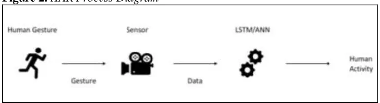
Human Activity Recognition

HAR is a thriving research topic in deep learning. In order to design an effective HAR system each of the steps of data acquisition must be considered. The steps are defined as: data acquisition from the sensor, pre -processing the data, feature extraction and training/classification an overview of the HAR process is shown in Figure 2. The dataset used in this problem was captured by making use of an android smartphone attached to the user’s body at which point they were asked to complete a list of 12 different human activities that make up each of our classes and is available at (Dua and Karra Taniskidou 2017). The performance of any HAR research will be affected by the techniques used at each of the activity recognition process steps. Moreover, in any monitoring system the performance will be greatly affected by the sensor used (Hassan et al. 2017).

The experiments were carried out, using 30 volunteers with ages between 19 and 48. Each volunteer performed the twelve activities that included: walking, standing, sitting, walking upstairs, walking downstairs, laying, standing to sitting, sitting to standing, sitting to laying, laying to sitting, standing to laying and laying to standing whilst the smartphone was attached to their waist. The experiments were all recorded in order to make the process of labelling the activities easier. The chosen smartphone for the experiments was a Samsung Galaxy S2 smartphone as it contains both an accelerometer and a gyroscope that helps capture angular velocity and 3-axial linear acceleration at a constant 50Hz this sampling rate is high enough to accurately capture the change in movements during the human activity. The following sections describe the signal processing of the data and any filtering used on the raw signals. The resulting dataset was divided up in to two different sets 70% was described as the training data set for training the model whereas the remaining 30% was used as the test data in order to validate the trained model (Reyes-Ortiz et al. 2012).

Signal Processing

The incoming gyroscope and accelerometer was put through many stages of pre-processing before it was input in to the training model. Noise was reduced by making use of both a median and third order low pass Butterworth filter. The filter has a cut off frequency of 20Hz. The frequency threshold was selected as literature describes that the energy spectrum of the human body lies in the range between 0 Hz and 15 Hz. Following this pre-processing we obtained a triaxial acceleration signal that was clean. The clean signal can also be conveyed as the summation of two acceleration vectors which can be named as gravitational component G and BA which is the body motion acceleration. These signals were segmented making use of another low pass filter with an optimal cut off of 0.3 Hz (Reyes-Ortiz et al. 2014).

After segmentation, the signals were divided up using fixed-width sliding windows; each window has a span of 2.56s with a 50% overlap (Reyes-Ortiz et al. 2016).

Human Activity Recognition on Given Dataset

Problem Domain

Detecting human activities making use of gyroscope readings poses many challenges due to the inconsistency of the data, therefore introducing interclass variability in to the dataset. For example, the action of sitting to standing and then standing to sitting can be different in different environments and between different users. Moreover, human behaviour changes and multiple tasks can be completed simultaneously therefore making it harder to correctly recognise an activity.

learning techniques to create a reliable and robust model of human activity recognition.

LSTM Design

The data was divided up in to training and validation data in a 70:30 split. Preliminary visualisation of the data showed that there were different general trends and patterns for different activities although there was variability between gyroscope data of the same class.

The LSTM model for the experiments was developed making use of the Keras LSTM (Brownlee 2017) classifier with all of the code written in python. Repeated 10-fold cross validation was used in order to effectively evaluate the classifier. Figure 3 shows how cross validation is applied to a system over each iteration.

Keras

Francois Chollet (a Google engineer) developed and maintains Keras. Keras is a python library for deep learning capable of using multiple backends. It was developed in order to make it fast and easy to develop models and complete research on different techniques. It is designed to run on any version of python later than 2.7 however it is recommended to run on version 3.5. It can run on any GPU with only a small amount of set up required (Keras 2018).2

Tensorflow

A Tensorflow environment in order to make use of Kera’s deep learning classifiers was used for this research. Tensorflow is a ML framework developed by Google. It is the second one they have developed, it is used to build, test and train different deep learning models. Tensorflow can be used to complete complex numerical computations making use of dataflow graphs (Tensorflow 2018).

K Fold Cross Validation

In k-fold cross-validation the original dataset is partitioned randomly into equal sizes, the number of these partitions is defined by the K variable. The data is then further divided so that a single K sample of the data is retained and kept unseen; this is used as the validation data for testing the model. The remaining K-1 subsets are used as the main training data. This cross-validation process can then be repeated K number of times (the folds) with each different K sub sets used once as the validation data. This has many advantages over other validation techniques as all of the observations are made making use of both the training and validation data at the same time. Furthermore, each validation set is used exactly once means that the models are not just trained for the same test and train data sets. Figure 3 shows how the data for each fold is partitioned for each fold.

Stratified K-fold cross validation was introduced to try and combat datasets that are not evenly balanced between the different classes. Each fold is selected so that each fold contains a similar proportion of class labels.

Repeated cross-validation repeated the cross-validation n number of times. With n random portions of the original sample yielded. The n results are then averaged out in order to produce a singular estimation of the model (Brownlee 2018).

Figure 3. Cross Validation Model

Results

Figure 4. Histogram of Activities and Postural Transitions

matrices are used to analyse the results. A fourth test was introduced to combat the imbalanced data by grouping together all of the postural transitions. Figure 4 shows a histogram of the different classes, with classes 1-6 representing standard activities and classes 7-12 are the postural transitions. It can be clearly seen that the data set contains significant class imbalance towards the standard activities. Reyes-Ortiz et al. (2016) balance the data by grouping together all of the postural transitions; however, for the purposes of these experiments we will keep them apart.

Each experiment comprised of a consistent number of epochs with varying number of neurons, the details of which can be read in Table 1.

Table 1.Number of Epochs and Neurons per Experiment

Number of Epochs Number of Neurons Number of Classes

Experiment 1 50 350 12

Experiment 2 50 100 12

Experiment 3 50 10 12

Each experiment was completed by using cross validation methods as described previously. Each test used ten-fold cross validation, with the best loss and accuracy per fold reported below. It is evident that the accuracy and the loss of the model improve as the number of neurons increases, with 350 LSTM neurons providing the best results. The accuracies presented represent the classification accuracies for each of the 12 different classes that were considered. It is important to note that these values will change for each iteration of the test as the NN does not always follow the same path. Tables 2 and 3 present the average performance for each test and the results from each fold. It can be seen that there is a clear trade-off between the time taken to train the model and the number of neurons used. As a direct result, it can be considered that continual training or online training of the model as outlined in Reyes-Ortiz et al. (2014) could be an acceptable way to improve the accuracy.

Table 2. Best Accuracy and Best Loss per Fold in Each Different Test

Experiment 1 Experiment 2 Experiment 3 Fold Accuracy Loss Accuracy Loss Accuracy Loss

1 0.94723 0.19128 0.91892 0.21641 0.82368 0.51748

2 0.93179 0.18562 0.90991 0.22369 0.75933 0.60864

3 0.92921 0.19149 0.90090 0.24912 0.77477 0.57704

4 0.94080 0.18151 0.91763 0.23443 0.72844 0.69128

5 0.95882 0.12116 0.93694 0.21028 0.75289 0.64023

6 0.92798 0.18684 0.93308 0.19595 0.75289 0.64865

7 0.94594 0.16575 0.91634 0.24413 0.79794 0.56883

8 0.91366 0.20554 0.90077 0.26693 0.75902 0.60082

9 0.94459 0.18222 0.90980 0.23877 0.81959 0.50970

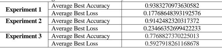
Table 3. The Average Best Loss and Accuracy

Experiment 1 Average Best Accuracy 0.9383270973630582

Average Best Loss 0.17768648393192576

Experiment 2 Average Best Accuracy 0.9142482320317372

Average Best Loss 0.23466352699422233

Experiment 3 Average Best Accuracy 0.7768827370225013

Average Best Loss 0.5927918261168678

Results presented in Reyes-Ortiz et al. (2013b) have shown that they can accurately determine HA with an overall 96% accuracy making use of SVM. These results are comparable to those obtained from the tests completed; however, they have introduced two alternative classes: a class of unknown – where the SVM cannot accurately predict the class - and a class where they have grouped together all of the postural transitions.

Confusion Matrix Experiment 1

Table 4. Confusion Matrix without Normalisation for Experiment 1

T ru e V a lu es

Walking 1211 8 7 0 0 0 0 0 0 0 0 0 Walking

Upstairs 30 1013 25 0 1 0 3 0 1 0 0 0 Walking

Downstairs 16 30 941 0 0 0 0 0 0 0 0 0 Sitting 1 0 1 1150 136 2 1 0 2 0 0 0 Standing 0 1 0 116 1305 0 0 1 0 0 0 0 Laying 0 0 0 0 0 1407 0 0 0 4 1 1 Standing

to sit 0 6 2 1 0 0 31 3 0 0 4 0 Sit to

Stand 1 0 0 1 0 0 3 12 3 1 2 0 Sit to Lie 0 0 0 2 0 1 1 2 42 2 24 1 Lie to Sit 0 0 0 0 0 2 0 0 2 37 4 15

Stand to

Lie 1 4 1 1 1 2 4 1 26 2 46 1 Lie to

Stand 0 0 0 0 0 3 0 0 5 25 1 23

Confusion Matrix Experiment 2

Table 5. Confusion Matrix without Normalisation for Experiment 2

T ru e V a lu es

Walking 1195 21 10 0 0 0 0 0 0 0 0 0

Walking Upstairs

61 959 45 0 2 0 5 0 0 0 1 0

Walking Downstairs

27 45 914 0 0 0 0 0 0 0 1 0

Sitting 0 0 1 1119 165 5 0 0 1 0 2 0

Standing 2 5 0 121 1295 0 0 0 0 0 0 0

Laying 0 0 0 0 0 1406 0 0 0 6 0 1

Standing to sit

3 7 2 0 2 0 26 4 0 0 3 0

Sit to Stand 1 1 0 1 0 0 5 7 5 0 3 0

Sit to Lie 0 0 2 0 0 0 1 2 44 1 23 2

Lie to Sit 0 0 0 1 0 5 0 0 4 26 5 19

Stand to Lie 1 11 5 0 1 1 3 1 28 1 35 3

Lie to Stand 0 0 0 1 0 2 0 0 1 21 4 28

W a lk in g W a lk in g U p st a ir s W a lk in g D o w n st a ir s S it ti n g S ta n d in g L a y in g S ta n d in g t o s it S it t o S ta n d S it t o L ie L ie t o S it S ta n d t o L ie L ie t o S ta n d Predicted Values

Confusion Matrix Experiment 3

Table 6. Confusion Matrix without Normalisation for Experiment 3

T ru e V a lu es

Walking 737 283 206 0 0 0 0 0 0 0 0 0

Walking Upstairs

157 780 118 2 12 0 0 0 2 0 2 0

Walking Downstairs

212 109 666 0 0 0 0 0 0 0 0 0

Sitting 3 1 0 1084 197 8 0 0 0 0 0 0

Standing 8 10 0 137 1268 0 0 0 0 0 0 0

Laying 0 0 0 0 0 1403 0 0 0 7 0 3

Standing to sit

32 11 0 1 3 0 0 0 0 0 0 0

Sit to Stand 12 2 0 1 1 1 0 0 6 0 0 0

Sit to Lie 20 4 2 12 0 0 0 0 33 2 0 2

Lie to Sit 0 1 0 2 0 17 0 0 7 14 0 19

Stand to Lie 38 15 9 2 1 1 0 0 20 3 0 1

Lie to Stand 0 0 0 1 0 16 0 0 8 15 0 17

Tables 4, 5 and 6 represent the confusion matrices of each the LSTM model for different experiment respectively. Because of the significant class imbalance (as shown in Figure 4) there is lots of confusion around the postural transitions. This is because there is not enough data to accurately train the model to identify these classes. In order to combat this and see if the results could be further improved, the postural activities were grouped together as done in Reyes-Ortiz et al. (2016) - giving only 7 classes in total.

Grouping Postural Transitions

Using the same parameters as the most accurate model (experiment 1, all of the postural transitions were grouped into a singular class. Therefore, seeing the effects of an LSTM model comparing it directly with those completed in literature under similar conditions. Table 7 shows the LSTM parameters used and the number of training epochs and number of classes.

Table 7. Number of Epochs and Neurons for Grouped Experiment

Number of Epochs Number of Neurons Number of Classes

Experiment 4 50 350 7

The classification results on the HAR dataset when postural transitions are grouped together are shown in Table 8 and Table 9. They show an average best loss of 0.1430 and an average accuracy of 0.95% using 10-fold cross validation. This is comparable to the work completed by Reyes-Ortiz et al. (2013a).

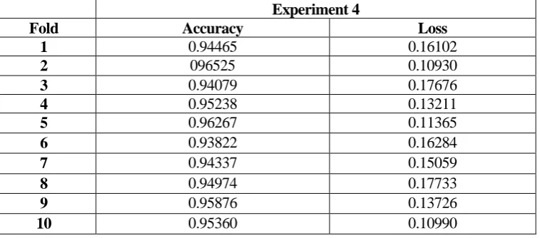
Table 8. Best Accuracy and Best Loss per Fold in during Group Postural Transition Training

Experiment 4

Fold Accuracy Loss

1 0.94465 0.16102

2 096525 0.10930

3 0.94079 0.17676

4 0.95238 0.13211

5 0.96267 0.11365

6 0.93822 0.16284

7 0.94337 0.15059

8 0.94974 0.17733

9 0.95876 0.13726

10 0.95360 0.10990

Table 9. Average Best Accuracy & Average Best Loss for Experiment 4 over the 10 Folds

Experiment 4 Average Best Accuracy 0.9509475049500213

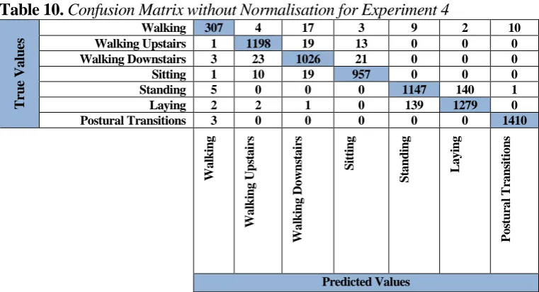
Comparing the confusion matrix for grouped postural transitions (Table 10) to those shown in Tables 4, 5, and 6 demonstrates that the grouping of postural transitions reduces the misclassifications shown in the confusion matrices. It is clear that the number of false positives and true positives has been greatly reduced.

The results obtained and detailed in Table 9 and Table 10 have been shown to outperform Karantonis et al. (2006) as their work which makes use of special purpose sensors has produced accuracies in the range of 90%-96%. Our work has shown accuracy in the range 93%-96%, and moreover it is more convenient to carry a smartphone that have bespoke sensors than sensors attached to different parts of the body. Similarly the work completed by Hanai et al. (2009) where a chest mounted accelerometer was used to record the HA has achieved an accuracy of 90.8% which is not as good as our results obtained using smartphone data. The argument for use of smartphones to for HAR is greatly increased as a direct result of these tests as on all occasions we have either outperformed or produced comparable results to those with bespoke sensors worn on the body.

Table 10. Confusion Matrix without Normalisation for Experiment 4

T ru e V a lu es

Walking 307 4 17 3 9 2 10

Walking Upstairs 1 1198 19 13 0 0 0

Walking Downstairs 3 23 1026 21 0 0 0

Sitting 1 10 19 957 0 0 0

Standing 5 0 0 0 1147 140 1

Laying 2 2 1 0 139 1279 0

Postural Transitions 3 0 0 0 0 0 1410

W a lk in g W a lk in g U p st a ir s W a lk in g D o w n st a ir s S it ti n g S ta n d in g L a y in g P o st u ra l T ra n si ti o n s Predicted Values Device Utilisation

Table 11. Device Utilisation Table

Device Utilisation

Epochs Used 350

Time Per Epoch (s) 14

Times Repeated Cross Validation: 10

NVIDIA INFORMATION GeForce GTX1050

Conclusions & Further Work

techniques to classify both standard activities and postural transitions. The final model proposed considers the trade-offs of the time needed to train the model against the performance of the classifier. This paper then also compares the proposed model with existing literature.

The scope of the work is to apply existing technology to real world situations whilst still maintaining comparable results but improving processing times and use of the systems resources. The continual development of this research could then be applied to a wide range of industries including: the military, assisted living facilities and health & fitness tracking.

The results of the experiments confirm that is possible to make use of LSTM classifiers to correctly identify human activities, although further experimentation should be completed to evaluate the model with more representative conditions (such as a smartphone held by a user under real-world conditions throughout the day). These tests would allow further refinement of the model.

Acknowledgments

This study has been carried out with the help and support of the ACES and C3RI faculties within Sheffield Hallam University who have allowed the use of their equipment and space.

References

Brownlee J (2017) How to Tune LSTM Hyperparameters with Keras for Time Series Forecasting. [Online]. [Accessed 12/4/2017]. https://bit.ly/2LpXIH2.

Brownlee J (2018) A Gentle Introduction to K-Fold Cross Validation. [Online]. [Accessed 23/5/2018]. https://bit.ly/2BxuR0k.

Coley B, Najafi B, Aminian K (2005) Stair Climbing Detection during Daily Physical Activity using a Miniature Gyroscope. Gait & Posture 22(4):287-294.

Dua D, Karra Taniskidou E (2017) UCI Machine Learning Repository. [Online]. http://archive.ics.uci.edu/ml/index.php.

Ermes M, Parkka J, Cluitmans M (2008) Advancing from Offline to Online Activity Recognition with Wearable Sensors. IEEE Engineering in Medicine and Biology Society Conference (Feb): 4451-4.

Hanai Y, Nishimura J, Kuroda T (2009) Haar-Like Filtering for Human Activity Recognition using 3D Accelerometer. Digital Signal Processing Workshop and 5th IEEE Signal Processing Education Workshop. DSP/SPE 2009. 13th IEEE.

Hardwick T (2018) Apple Watch Owners can Compete in WatchOS 5, Auto-Detection of Workouts Coming Too. [Online]. [Accessed 4/6/2018]. https://bit.ly/2UYw5JA. Hassan M, Uddin M, Mohamed A, Almogren A (2017) A Robust Human Activity

Recognition System using Smartphone Sensors and Deep Learning. Future Generation Computer Systems 81(Apr): 307-313.

Karantonis DM, Narayanan MR, Mathie M, et al. (2006) Implementation of a Real-Time Human Movement Classifier using a Triaxial Accelerometer for Ambulatory Monitoring. IEEE Transactions on Information Technology in Biomedicine10(1). Khan A, et al. (2010) Human Activity Recognition via an Accelerometer-Enabled

Smartphone using Kernal Discriminant Analysis. International Conference on Future Information Technology.

Liu J, Shahroudy A, Xu D, Wang G (2016) Spatio-Temporal LSTM with Trust Gates for 3D Human Action Recognition. In Computer Vision – ECCV 2016.Lecture Notes in Computer Science 9907. Edited by Leibe B, Matas J, Sebe N, Welling M. Springer. Maurer U, et al. (2006) Activity Recognition and Monitoring Multiple Sensors on

Different Body Positions. IEEE International Workshop on Wearable and Implantable Body Sensor Networks 4.

Reyes-Ortiz J, et al. (2012) Human Activity Recognition on Smartphones using a Multiclass Hardware-Friendly Support Vector Machine. 4th International Workshop of Ambient Assisted Living 216.

Reyes-Ortiz J, et al. (2013a) Energy Efficient Smartphone-Based Activity Recognition using Fixed-Point Arithmetic. Journal of Universal Computer Science 19(9).

Reyes-Ortiz J, et al. (2013b)A Public Domain Dataset for Human Activity Recognition Using Smartphones. In ESANN.

Reyes-Ortiz J, et al. (2014) Human Activity Recognition on Smartphones with Awareness of Basic Activities and Postural Transitions. In ICANN.

Reyes-Ortiz J, et al. (2016) Transition-Aware Human Activity Recognition using Smartphones. Neurocomputing 171(Jan): 754-767.

Srivastava P (2017) Introduction to Long Short-Term Memory. [Online]. [Accessed 10/12/2017]. https://www.analyticsvidhya.com/blog/2017/12/fundamentals-of-deep-learning-introduction-to-lstm/.

Staudemeyer R, Omlin C. (2016) Evaluating Performances of Long Short-Term Memory Recurrent Neural Network on Intrusion Detection Data. SAICSIT '13 Proceedings of the South African Institute for Computer Scientists and Information Technologists Conference. East London, South Africa.