Efficiently measuring a quantum device using machine learning

Efficiently measuring a quantum device using machine

learning

D. T. Lennon†1, H. Moon†1, L. C. Camenzind2, Liuqi Yu2, D. M. Zumb¨uhl2, G. A .D. Briggs1, M. 1

A. Osborne3_{, E. A. Laird}4 _{& N. Ares}1 2

1_{Department of Materials, University of Oxford, Parks Road, Oxford OX1 3PH, United Kingdom} 3

2_{Department of Physics, University of Basel, 4056 Basel, Switzerland} 4

3_{Department of Engineering, University of Oxford, Parks Road, Oxford OX1 3PJ, United Kingdom} 5

4_{Department of Physics, Lancaster University, Lancaster, LA1 4YB, United Kingdom} 6

Scalable quantum technologies such as quantum computers will require very large num-7

bers of quantum devices to be characterised and tuned. As the number of devices on chip 8

increases, this task becomes ever more time-consuming, and will be intractable on a large 9

scale without efficient automation. We present measurements on a quantum dot device per-10

formed by a machine learning algorithm in real time. The algorithm selects the most infor-11

mative measurements to perform next by combining information theory with a probabilis-12

tic deep-generative model that can generate full-resolution reconstructions from scattered 13

partial measurements. We demonstrate, for two different current map configurations that 14

the algorithm outperforms standard grid scan techniques, reducing the number of measure-15

ments required by up to 4 times and the measurement time by 3.7 times. Our contribution 16

goes beyond the use of machine learning for data search and analysis, and instead demon-17

learning-based automated measurement of quantum devices. 19

Introduction 20

Semiconductor quantum devices hold great promise for scalable quantum computation. In par-21

ticular, individual electron spins in quantum dot devices have already shown long spin coherence 22

times with respect to typical gate operation times, high fidelities, all-electrical control, and good 23

prospects for scalability and integration with classical electronics1. 24

A crucial challenge of scaling spin qubits in quantum dots is that electrostatic confinement 25

potentials vary strongly between devices and even in time, due to randomly fluctuating charge traps 26

in the host material. Characterising such devices, which requires measurements of current or con-27

ductance at different applied biases and gate voltages, can be very time consuming. It is normally 28

carried out following simple scripts such as grid scans, which are sequential measurements taken 29

from a 2D grid for a pair of voltages. We call a set of voltages that defines the state of a quantum 30

dot a configuration. Measurement of some configurations is more informative for characterising a 31

quantum dot than the other configurations; measuring uncertain signals is more informative than 32

measuring predictable signals. However, grid scans do not prioritise measurement of informative 33

signals, instead just acquiring measurements according to simple rules (e.g. following a raster pat-34

tern). Current efforts in the field of automation of quantum dot are focused on tuning2–9_{, a large} 35

portion of these relying on grid scanning techniques for measurement. An optimised measurement 36

method that can prioritise and select important configurations is thus key for fast characterisation 37

and holds the potential to increase the efficiency of these approaches when combined. 39

In this paper, we present an algorithm that performs efficient real-time data acquisition for 40

a quantum dot device (Fig. 1a). It starts from a low-resolution uniform grid of measurements, 41

creates a set of full-resolution reconstructions, calculates the predicted information gain (i.e. the 42

acquisition map), selects the most informative measurements to perform next, and repeats this 43

process until the information gain from new measurements is marginal. 44

In order to select measurements based on information theory, we require a corresponding 45

uncertainty measure (of random variables)10–12, and hence a probabilistic model of unobserved 46

variables. One typical approach is to use a Gaussian process13_{. Here, we use a conditional} vari-47

ational auto-encoder (CVAE) 14, which is capable of generating high-resolution reconstructions 48

given partial information and is fast enough for real-time decisions. Deep generative models such 49

as adversarial networks (GAN)15_{, the variational auto-encoder (VAE)}16 _{and its extensions, such} 50

as CVAE, have shown great success in multi-modal distributions and complex non-stationary pat-51

terns of data17, 18_{, similar to those of observed in quantum device measurements. These are the} 52

main advantages of CVAE over a basic Gaussian process. Also, CVAE is more computationally 53

efficient at generating multiple full-resolution reconstructions. Although progress has been made 54

addressing the limitations of Gaussian processes, deep generative models are overall a better fit to 55

the requirements for efficient quantum device measurements. Deep generative models have been 56

used for: speech synthesis19; generating images of digits and human faces20, 21; transferring image 57

scientific research to optimise molecular structures25–28. In spite of their suitability, these models 59

have not previously been applied to efficient data acquisition. An advantage of deep generative 60

models over simple interpolation techniques, such as nearest-neighbour and bilinear interpolation, 61

is that deep generative models can learn likely patterns from training data and incorporate them 62

into its reconstructions. Our method, as it is data-driven, it is generalizable to different transport 63

regimes, measurement configurations, and more complex device architectures if an appropriate 64

training set is available. 65

Results 66

The device Our device is a laterally defined quantum dot fabricated by patterning Ti/Au gates 67

over a GaAs/AlGaAs heterostructure containing a two-dimensional electron gas (Fig. 1b). In this 68

device, electrons are subject to the confinement potential created electrostatically by gate voltages. 69

Gate voltagesV1toV4tune the tunneling rates whileVGmainly shifts the electrical potential inside 70

the quantum dot. The current through the device is determined both by these gate voltages and by 71

the bias voltageVbias. Measurements were performed at30mK. 72

The quantum dot is characterised by acquiring maps of the electrical current as a function of a 73

pair of varied voltages, which we call a current map configuration. We first focus on varyingVGand 74

Vbias for fixed values ofV1 toV4. Figure 1c) shows a typical example. Diamond-shaped regions or 75

‘Coulomb diamonds’ indicate Coulomb blockade, where electron tunnelling is suppressed29. Most 76

ments in these regions slow down informative data acquisition. Our algorithm must therefore give 78

measurement priority to the informative regions of the map. An overview of an algorithm-assisted 79

measurement of a current map is shown in Fig. 1d. 80

Training the reconstruction model The role of the reconstruction model is to characterise likely 81

patterns in a training data set, given by a mixture of measured and simulated current maps. We can 82

utilise these likely patterns to predict the unmeasured signals from partial measurements. 83

Deep generative models represent this pattern characterisation in a low-dimensional real-84

valued latent vector z, which can be decoded to produce a full-resolution reconstruction. The 85

latent space representation and the decoding are learned during training. Our CVAE consists of 86

two convolutional neural networks, an encoder and a decoder. The encoder is trained to map full-87

resolution training examples of current mapsY to the latent space representationz. The encoder 88

also enforces that the distributionp(z)of training examples in latent space is Gaussian. 89

The decoder is trained to reconstruct Y, from the representationzcombined with an8×8

90

subsample ofY. As a result,zattempts to represent all the information that is missing from the 91

subsampled data. In a plain VAE, the input of a decoder is onlyz. If a decoder takes additional 92

input exceptz, then it is called CVAE, and we found that CVAE generates better reconstructions 93

than VAE for the considered measurements. The chosen loss function, which the CVAE tries to 94

minimise, is a measure of the difference between the training data and the corresponding recon-95

struction. To avoid blurry reconstructions, we define a contextual loss function that incorporates 96

descrip-(i)

(ii)

(iii)

(iv) a

c

Vbias

VG

b

d

V2

VG

V1

Vbias

V3

V4

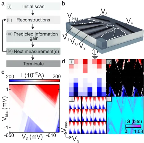
Figure 1: Overview of the algorithm and the quantum dot device. a, Schematic of the

al-gorithm’s operation. Low-resolution measurements (i) are used to produce reconstructions (ii),

which are used to infer the predicted information gain acquisition map (iii). Based on this map,

the algorithm chooses the location of the next measurement (iv). The process is repeated until a

stopping criterion is met.b, Schematic of the device. A bias voltageVbiasis applied between ohmic

contacts to the two-dimensional electron gas. We apply gate voltages labelledV1toV4andVG. c, A

measured current map as a function ofVbiasandVG. The Coulomb diamonds are the white regions

where electron transport is suppressed, and most of the information necessary to characterise a

device is contained just outside these diamonds. d, Sequential decision algorithm inaillustrated

with an example of a specific current map. In panel (iv), unmeasured pixels are plotted in black;

however, initial measurements (i) are represented so as to fill the entire panel (that is, the sparse

tion of these networks and their training can be found in the Supplementary sections Training and 98

loss function, and Network specification. 99

The model is trained using both simulated and measured current maps. We choose to work 100

with current maps of resolution128×128. The simulation is based on a constant-interaction model 101

(see Methods). To measure the current maps for training, we set the bias and gate voltage ranges 102

randomly from a uniform distribution. The training data set consists of 25,000 simulations and 103

25,000 real examples generated by randomly cropping 750 measured current maps. The current 104

maps were subjected to random offsets, rescaling, and added noise to increase the variability of the 105

training set. 106

Generating reconstructions from partial data After training, only the trained decoder network 107

is used in the algorithm of Fig. 1a to reconstruct full-resolution current maps from partial data. 108

At each stage, the known partial current map is denoted Yn, where n ≤ 1282 = 16,384 is the

109

number of pixels to be measured. To generate a reconstruction, the decoder takes as input the 110

initial8×8grid scanY64, together with a latent vectorzsampled from the posterior distribution 111

p(z|Yn)(see Methods for detail equations and Fig. S1 for the decoder diagram). Note that the

pos-112

terior density is calculated by the prior densityp(z)and a likelihood function, which is comparing 113

reconstructions and the partial data. Multiple posterior samples are drawn from p(z|Yn) by the

114

Metropolis-Hastings (MH) method to approximatep(z|Yn). From these multiple sampleszm,

cor-115

responding reconstructions are then generated, denotedYˆm. In this paper we setm = 1, . . . ,100.

116

The continuous posteriorp(z|Yn)is then approximated by a discrete posterior of samplesPn(m),

which denotes how probableYˆm is. We refer toPn(m)as the posterior distribution of

reconstruc-118

tions. 119

Making measurement decisions With each iteration of the decision algorithm, an acquisition 120

map is computed from the accumulated partial measurements and the resulting reconstructions. 121

This acquisition map assigns to each potential measurement location (i.e. to each pixel location 122

in the current map) an information value for the posterior distribution of reconstructions (Fig. 2). 123

The(n+ 1)th measurement, whose result isyn+1, is one pixel taken from the true current map and 124

changes our posterior distribution from Pn(m) to Pn+1(m), rendering different reconstructions 125

more or less probable. 126

The acquisition map is the expected information gain IG(x)at each potential measurement 127

locationx. Our algorithm calculates it by a weighted sum over reconstructions: 128

IG(x)≡X m

Pn(m)×IGm x

, (1)

whereIGm(x) is the Kullback-Leibler divergence between the distributionsPn and Pn+1, calcu-129

lated such thatyn+1 at locationxis taken from reconstruction Ymˆ . The most informative point is 130

x∗_n+1 ≡ argmax_xIG(x). This criterion is equivalent both to minimising the expected information 131

entropy of the posterior distribution and to Bayesian active learning by disagreement (BALD10, 132

see Methods). The difference of the proposed method and BALD is that the proposed method uses 133

random reconstructions of data, which can be multi-modal, whereas BALD assumes that data is 134

I(pA)

IG (bits)

V (mV)G

x

x

b

V (mV)G

x

x

a

c d

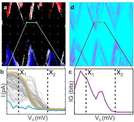
Figure 2: Computing the acquisition map. a, Partial current map. To illustrate the first step in

the computation of the acquisition map, we consider a trace (green) through an unmeasured region

of the map. b, For the unmeasured trace in a, reconstructions provide 100 different predictions.

Blue and yellow traces highlight two of these predictions. The objective is to determine the most

informative measurement location. Atx2, all predictions are similar, so measuring here will have

little impact on the posterior distribution of reconstructions. Atx1, predictions are dissimilar and

therefore x1 is a more informative measurement location, with a larger effect on the posterior

distribution of reconstructions. c, Information gain computed for the unmeasured trace in a. d,

Acquisition map of information gain computed from the partial measurements in a, and plotted

We devised two methods to make decisions based on the acquisition map; a pixel-wise 136

method, and a batch method. The pixel-wise method selects the single best location in the ac-137

quisition map. In practice, this is often not optimal in terms of measurement time, because it 138

does not take account of the time needed to ramp the gate voltage between measurement locations 139

(which is limited by details of the measurement electronics and the device settling time). To take 140

account of this limitation, we also devised a batch method, which selects multiple locations from 141

the acquisition map, and then acquires measurements by taking a fast route between them. This 142

reduces the measurement time compared with the pixel-wise method. 143

Experiments To test the algorithm, it was used to acquire a series of current maps in real time. 144

First, the device was thermally cycled, to randomise the charge traps and therefore present the 145

algorithm with a configuration not represented in its training data. Gate voltagesV1-V4 were set 146

to a combination of values, and the algorithm was tasked to measure the corresponding current 147

map using both the batch and the pixel-wise methods. This step was repeated for ten different 148

combinations of bias and gate voltages. Fig. 3 presents data acquired by the algorithm at selected 149

acquisition stages, together with selected reconstructions. As expected, reconstructions become 150

less diverse as more measurements are acquired. The reconstructions do not necessarily replicate 151

the measured current map for large n. This is because reconstructions have a limited variability 152

given by the training data. Decisions are made based on the learned patterns from the training 153

data, which implies that this training data should contain at least general patterns which are to be 154

n=64

n=512

n=2,048

n=4,096

n=8,192

n=16,384

n=64

n=512

n=2,048

n=8,192

n=16,384

Ŷ Yn

Figure 3: Updating reconstructions using information from new measurements. In each

row, the first column shows the algorithm-assisted measurements, using the batch method, for a

givenn. The remaining three columns contain example reconstructions given the correspondingn

measurements. As nincreases, the diversity of the reconstructions is reduced and their accuracy

increased. As expected, the uncertainty is almost eliminated in the last row. The residual remaining

As seen, the algorithm gives high priority to regions of the map where the current is rapidly 156

varying, and avoids regions of nearly constant current, such as the interiors of Coulomb diamonds. 157

This strategy is an emergent property of the algorithm and is wise; little information about the 158

device characteristics can be found in low-current gradient regions of the current map. This pref-159

erence derives from the comparison between reconstructions, which exhibit the greatest disagree-160

ment outside Coulomb diamonds. This is also seen in Fig. 4a, which shows two representative 161

measurement sequences using the batch method. The batch method collects grouped measure-162

ments while the pixel-wise method distributes measurements more uniformly, given that in this 163

case, the acquisition map is more frequently updated to take account for recently acquired infor-164

mation. Results for other current maps, including for the pixel-wise method, are shown in the 165

Supplementary Figures 2 to 6. 166

We compared the performance of the algorithm with an alternating grid scan method. This 167

type of grid scan starts with 8×8 measurements and alternately increases the vertical and the hori-168

zontal grid size by 2 (i.e. 16×8, 16×16, 32×16, etc.), without performing the same measurement 169

twice. Over the ten different current maps, the average time for full-resolution data acquisition 170

with the alternating grid scan method is 554 seconds. This time is limited by our bias and gate 171

voltage ramp rate and chosen settling time. The batch method can be implemented with any batch 172

size however for direct comparison with the alternating grid scan we selected increasing batches 173

of 32×2b_{, wherebis the batch number starting from 1.}

174

structions using the MH method, and constructing the acquisition map. One MH sampling iteration 176

takes 63 ms. For experiments, multiple sampling iterations are performed after each batch decision 177

and measurement while acquisition is suspended. Since sampling can be performed simultaneously 178

with measurement acquisition, from now on our measurement times exclude the time for sampling. 179

To compute a single acquisition map takes approximately 50 ms using a NVIDIA GTX 1080 Ti 180

graphics card and Tensorflow30_{implementation. The acquisition map must be computed for every} 181

batch or every pixel measurement, except for the initial8×8 grid scan and the final acquisition 182

step (which has no choice of which pixel(s) to measure). To acquire a full resolution current map 183

thus requires 7 computations (350 ms) for the batch method, and 16,319 computations (816 s) for 184

the pixel-wise method. For the batch method, the computation time is negligible compared to the 185

measurement time, but for the pixel-wise method it is a limiting factor in the measurement rate. 186

To quantify the algorithm’s performance, we have devised a measure based on the observa-187

tion that the most informative regions of the current map are those where the current varies strongly 188

withVGandVbias. We therefore define the local gradient of the current map at each locationxas 189

v(x)≡ k∇Y(x)k2 =

s

∂I(x) ∂VG

2 +

∂I(x)

∂Vbias

2

, (2)

whereI(x)is current measurement atx, and the derivatives are calculated numerically. The error 190

measurer(n)of a partial current map is the fraction of the total gradient that remains uncaptured, 191

i.e. 192

r(n)≡1− V(n)

V(N) (3)

whereV(n) ≡Pn

n=512 n=1,024 n=2,048 n=4,096 n=8,192 n=256

a

Grid Optimal Batch Batch (est) c

b Vbias

VG

e d

0

v(x)

0 0.0021 v(x) 0.0007

0.0 1.0

r(n)

Measurement number n

4,096 8,192 16,384

64 0.0

1.0

r(n)

4,096 8,192 16,384

64

(a.u.)

(a.u.) Measurement number n

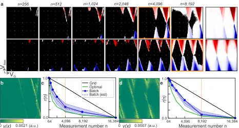
Figure 4: Measurements of Coulomb diamonds performed by the algorithm. a, Sequential

batch measurement in two different experiments. Each row displays algorithm assisted

measure-ments of the current map as a function ofVbias and VG for different values of n. The last plot in

each row is the full-resolution current map. b, d, Current gradient map (defined by Eq. (2)) for

each example ina. c, e, Measure of the algorithm’s performancer(n), real-time estimate ofr(n)

across reconstructions (with 90% credible interval shaded), and optimalr(n)for both examples in

a. The black line is the value ofr(n)corresponding to the alternating grid scan method. The

ver-tical orange line indicates the value ofndetermined by the stopping criterion. The corresponding

ment. This error can only be calculated after all measurements have been performed. However, 194

we can utilise the mth reconstruction to generate an estimate r˜m(n) in real time by replacing

195

k∇Y(x)k2withk∇Yˆm(x)k2. The estimates from multiple reconstructions yield a credibility inter-196

val forr(n). For an optimal algorithm, the error would ber(n) = 1.0¯ − V_V∗₍(_Nn₎), whereV∗(n)is the 197

sum of the largestn values of v(x). This would be achieved if each measurement location were 198

chosen knowing the full-resolution current map, and thus the location of the the highest unmea-199

sured current gradient. No decision method can exceed this bound. For the real time estimates of 200

r(n), we have increased the number of reconstructions to 3,000 by adding different noise patterns 201

that are present in typical measured current maps (see Supplementary section Noisy reconstruc-202

tion). This increase in the variability of the reconstructions is needed to avoid an overconfident 203

estimation ofr(n). 204

Performances for two experiments are shown in Fig. 4c, e. Grid scans reducer(n)linearly 205

with increasingn. The decision algorithm outperforms a simple grid scan and is nearly optimal. 206

When most of the current gradient is localised, the grid scan is far from optimal and even the 207

decision algorithm has room for improvement. In this case, the performance of the algorithm is 208

determined by how representative the training data is. Quantitative analysis of all 10 experiments 209

is in Supplementary Figures 5 and 6. 210

We propose a simple stopping criterion that uses the estimated reduction of the errorr(n)to 211

determine when to stop measuring a given current map, in a scenario where more experiments are 212

next measurement batch is estimated for reconstructionmto ber˜m(n+ ∆), where∆is the size of

214

the batch. Thus the estimated rate at which the error decreases isβm ≡

r˜_m(n+ ∆)−r˜_m(n)|/∆.

215

In the worst case among the candidate reconstructions, this rate is β ≡ minmβm. However, if

216

the algorithm begins to measure a new map, for which no reconstructions yet exist, the error of 217

that map will decrease at a rate of at least α ≡ 1/N; this is the slope achieved by a grid scan 218

and the worst case of the decision algorithm (black lines in Fig. 4c, e). Hence whenβ < α, it is 219

beneficial to halt measurement and move onto a new current map that is awaiting measurement. 220

Sinceαandβare the worst-case estimates for each case, the criterion is conservative. The stopping 221

points by this criterion are shown in Fig. 4c, e, with orange dashed lines. The total average time 222

(measurement time plus decision time) to reach the stopping criterion was 237 s, compared with 223

554 s to measure the complete current map by grid scan, reducing the time needed by a factor 224

between 1.84 and 3.70 across all 10 test cases. A more sophisticated stopping criterion utilising 225

the number of remaining unmeasured current maps and a total measurement budget is presented in 226

Methods. 227

Generalising the algorithm The algorithm described here does not require assumptions about 228

the physics of the acquired data, such as requiring that it show Coulomb diamonds. Provided that 229

training data are available, it should also work for other kinds of measurements. To test this, we 230

applied it to a different current map configuration also encountered in quantum dot tuning. In this 231

case the current flowing through the device is measured as a function of two gate voltages (V1 232

andV2), while keeping other voltages fixed (VG,Vbias,V3 andV4). In these current maps, Coulomb 233

current. For the training set, we measured 382 current maps with a resolution of251×251which 235

we randomly cropped to a resolution of128×128 and subjected to simple image augmentation 236

techniques (as for the previous training set). 237

We tested the performance of the algorithm in this new scenario by taking two different 238

combinations of VG, Vbias, V3 and V4 and measuring the corresponding current maps in real time 239

(Fig. 5). The device was thermally cycled after the training set was acquired and also between the 240

acquisition of the two current maps in Fig. 5. The algorithm focuses on measuring regions of high 241

current gradient, the corner edges and, in particular, the Coulomb peaks close to these. 242

In the top row of Fig. 5a,n= 4,096was chosen by the stopping criterion. In the bottom row, 243

the corners edges extended further in the current map and the stopping criterion chosen = 8,192. 244

This reduced the time needed to measure the current maps by 3.36 and 1.50, respectively, for the 245

two test cases when compared with the alternating grid scans. 246

Discussion 247

The proposed measurement algorithm makes real-time informed decisions on which measurements 248

to perform next on a single quantum dot device. Decisions are based on the disagreement of 249

competing reconstructions built from sparse measurements. The algorithm outperforms grid scan 250

in all cases, and in the majority of cases shows nearly optimum performance. The algorithm 251

reduced the time required to observe the regions of finite current gradient by factors ranging from 252

16,384 Measurements

64 4,096 8,192 0.0

1.0

Grid Optimal Batch Batch (est)

r(n)

Measurements

64 4,096 8,192 16,384 0.0

1.0

r(n)

n=512 n=1,024 n=2,048 n=4,096 n=8,192 n=256

a

c b

V2 V1

e d

0 0.0010

0v(x) 0.0015(a.u.) _v(x) (a.u.)

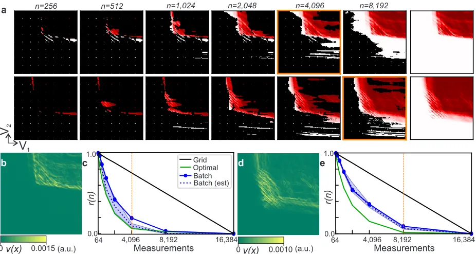
Figure 5: Measuring a different current map. a, Sequential batch measurement. Each row

displays the algorithm-assisted measurements of a current map as a function of V1 and V2 for

different values of n. The last plot in each row is the full-resolution current map. b, d, Current

gradient map for both examples ina. c, e, Measure of the algorithm’s performancer(n), average

real-time estimate ofr(n)with 90% credible interval, and optimalr(n)for both current maps ina.

The black line is the value ofr(n)corresponding to the alternating grid scan method. The dashed

orange line indicates the value of n determined by the stopping criterion. The corresponding

current map in ais highlighted in orange. The alternating grid scan took 2,267 s and 2,333 s to

acquire all measurements in the two cases. The batch method took 673 s and 1,552 s to reach the

further, however, the performance gain is limited by the spread of the information gain over the 254

scan range. This is evidenced in both Figs 4c,e and Fig 5c,e, where we show that even an optimal 255

algorithm does not significantly outperform the algorithm. 256

Our algorithm with no modifications can be re-trained to measure different current maps. It 257

simply requires a diverse data set of training examples from which to learn. The decision algorithm 258

performed well even when trained on a small data set of only 382 current maps (at a resolution of 259

251×251), implying that it is robust to limited training data sets. Our algorithm focused on observ-260

ing all informative regions present in the current map, making it generalisable to different types 261

of measurements and devices. The acquisition function can still be specifically designed to focus 262

on specific transport features such as Coulomb peaks or Coulomb diamond edges. In additional 263

experiments we demonstrate how this can be achieved by applying additional transformations to 264

the reconstructions (see Supplementary Section Context-aware decision for stability diagrams). 265

We believe that our algorithm represents a significant first step in automating what to measure 266

next in quantum devices. For a single quantum dot it provides a means of accelerating what can 267

currently be achieved by human experimenters and other automation methods. When provided 268

with an appropriate training data set our algorithm can be applied to a large variety of experiments. 269

In particular, in any conventional qubit tuning method for which time-consuming grid scans are 270

performed, our algorithm would allow for an improvement in measurement efficiency. It will not 271

be long before this kind of approach enables experiments to be performed, and technology to be 272

Methods 274

Distribution of reconstructions and sampling Since it is known that deep generative models 275

work well when the data range is from -1 to 1, all measurements are rescaled so that the maximum 276

value of the absolute value of the initial measurement is 1. LetY be a random vector containing 277

all pixel values. ObservationYn, wheren ≥ 1, is the set of pairs of locationxj and measurement

278

yj: Yn ={(xj, yj)|j = 1, . . . , n}. Also, a subset of measurements is defined:Yn:n0 ={(xj, yj)|

279

j =n, . . . , n0}. The likelihood of observations givenY is defined by 280

p(Yn|Y)∝exp −λΣ(x,y)∈Yn|y−Y(x)|

, (4)

whereY(x)is the pixel value ofY at x, andλis a free parameter that determines the sensitivity 281

to the distance metric and is set to 1.0 for all experiments in this paper. The posterior probability 282

distribution is defined by Bayes’ rule: 283

p(Y |Yn)∝p(Yn |Y)p(Y). (5)

Likewise, we can find the posterior distribution of z given measurements instead of Y. Let z0 284

denote another input of the decoder, which is set to Y64 in the experiments. Then the posterior 285

distribution ofzcan be expressed withz0whenn≥64: 286

p(z|Yn,z0)∝p(z|z0)p(Yn |p(z,z0)

∝p(z) Z

Y

p(Yn |Y)p(Y |p(z,z0)dY

∝p(z)p(Yn |Y = ˆYz),

where Yˆz is the reconstruction produced by the decoder given z and z0. Since all inputs of the

287

aszandz0 are assumed independent. Proposal distribution for MH is set to a multivariate normal 289

distribution having centered mean and a covariance matrix equal to one quarter of the identity 290

matrix. For the experiments in this paper, 400 iterations of MCMC steps are conducted when 291

n = 32×2b_{, whereb is any integer larger than or equal to 1. We found that 400 iterations result}

292

in good posterior samples. If (xn+1, yn+1) is newly observed, then the posterior can be updated 293

incrementally: 294

p(z|Yn+1,z0) =

p(xn+1, yy+1 |z,z0)

p(xn+1, yn+1|Yn,z0)

p(z|Yn,z0)

= p(xn+1, yy+1 | ˆ Yz)

p(xn+1, yn+1|Yn,z0)

p(z|Yn,z0),

because each term in (4) can be separated. 295

Decision algorithm In this section, we derive a computationally simple form of the information 296

gain and the fact that maximising the information gain is equal to minimising the entropy. Let 297

pn(·) = p(·|Yn,z0), and any probabilistic quantity of yn+1 has the conditionxn+1, but omitted for 298

brevity. 299

The continuous version of the information gain equation is

Eyn+1 h

KL pn(z|yn+1)kpn(z) i

= Z

yn+1

pn(yn+1)KL pn(z|yn+1)kpn(z)

dyn+1

= Z

yn+1

pn(yn+1)

Z

z

pn(z|yn+1) log

pn(z|yn+1)

pn(z)

dzdyn+1 (6)

= Z

yn+1 Z 0

z

pn(z, yn+1) log

pn(z, yn+1)

pn(z)pn(yn+1)

dzdyn+1

where KL is Kullback-Leibler divergence, I(·;·) is mutual information. Since I(z | Yn; yn+1 | 300

Yn) = H(z | Yn)−H(z | Yn, yn+1), maximising the expected KL divergence is equivalent to 301

minimisingH(z|Yn, yn+1), which is the entropy ofzafter observingyn+1. 302

Since this integral is hard to compute, we approximate probability density functions (PDFs) 303

with samples and substitute them into (6). Letnsdenote the number of measurements that are used

304

for sampling reconstructionszˆ1, . . . ,ˆzM (the samples are converted toYˆ1, . . . ,YˆM). Thenpns(z)≈

305

1

M P

mδˆzm(z), or with the sample indexm, Pns(m) = 1/M. For any n ≥ ns, the probability is

306

updated with the new measurements afterns: Pn(m;ns) =

p(Yns+1:n|Yˆm)

Σmp(Yns+1:n|Yˆm), which can be derived

307

from importance sampling. For brevity, the sampling distribution information ns is omitted for

308

the remaining section. Likewise,pn(yn+1) =

R

zpn(yn+1 | z)pn(z) ≈

P

mPn(m)pn(yn+1 | zm).

309

Lastly, we use the value of Yˆm at xn+1 for a sample of pn(yn+1 | zm) for simple and efficient

310

computation. As a result, the information gain is approximated by: 311

Eyn+1 h

KL pn(z|yn+1)kpn(z) i

≈X

m

Pn(m)KL(Pn+1kPn).

Simulator for Training data To aid the training of the model simulated training data was used to 312

prevent over-fitting. Simulated data produced via a simple implementation of the constant inter-313

action model29 _{was used along with basic data augmentation techniques. These techniques were} 314

not intended to be physically accurate but instead to produce quickly a diverse set of examples that 315

electrons within the dot can be captured by a simple constant capacitance CΣ which is given by 318

CΣ = CS +CD +CG where CS, CD and CG are capacitances to the source, drain and gate re-319

spectively. Making this assumption the total energy of the dot U(N)where N is the number of 320

electrons occupying the dot, isU(N) = (−|e|(N−N0)+CSVS+CDVD+CGVG)2

2CΣ +

N P

n=1

EnwhereN0 compen-321

sates for the background charge andEn is a term that represents occupied single electron energy

322

levels that is characterised by the confinement potential. 323

Using this we derive the electrochemical potential µ(N) = U(N)−U(N −1) = e2 CΣ(N −

324

N0− 1₂)−

|e|

CΣ(VSCS+VDCD+VGCG) +En.

325

To produce a training example random values are generated forCS,CDandCG. The energy 326

levels within a randomly generated gate voltage window and source drain bias window are then 327

counted. To aid generalisation to real data we randomly generated energy level transitions (which 328

are also counted) as well as slightly linearly scaledCΣ,CS,CD, andCGwithN. This linear scaling 329

was also randomly generated and results in produced diamonds that vary in size with respect toVG. 330

Examples of the training data produced by this simulator can be seen in Supplementary Figure 1. 331

Stopping criterion Utility, denoted byu, is the ratio of total measured gradient to the total gra-332

dient of a stability diagram: u(n) = 1.0−r(n). Here, we assume that we haveK more stability 333

diagrams to be measured. The location of each diagram is defined by a different voltage range, and 334

k = 0, . . . , K is the index of the diagrams, wherek = 0 is the index of the diagram that we are 335

currently measuring. 336

In this paper we assume that a unit budget for measuring one pixel is 1.0. The total utility is 338

utot=

K X

k=0

uk(tk)

=u0(t0) +unxt(T −t0),

where uk(·) is the utility from measuring kth diagram, tk is the planned budget for kth diagram

339

satisfyingPK

k=0tk =T, andunxt(T −t0) =PK_k=1uk(tk). 340

Lettdenote the already spent budget on the current diagram,t ≤t0. If we stop the measure-341

ment thent0 =t, ort0 =t+ ∆if we decide to continue the measurement, where∆is a predefined 342

batch size. For the decision, the utilities of two cases are compared: whent0 =t, 343

utot=u0(t) +unxt(T −t). (7)

Otherwise,t0 =t+ ∆and 344

utot=u0(t+ ∆) +unxt T −(t+ ∆)

. (8)

If (8)<(7), it is better to stop and move to the next voltage range. Rearranging the inequality leads 345

to 346

u0(t+ ∆)−u0(t)< unxt(T −t)−unxt T −(t+ ∆)

. (9)

The left-hand-side (lhs) of (9) means the difference of utility if we invest ∆budget more on the 347

current diagram, and the right-hand-side the difference when∆more budget is used for remaining 348

diagrams. As we discussed in Results section, we can calculate multiple slope estimates βm for

349

spending∆to the current diagram: u0(t+ ∆)−u0(t)≈βm∆.

The right-hand-side (rhs) of (9) can be approximated byα∆ifK =∞, whereα= 1/16,384

351

is the slope of grid scan measuring a new stability diagram. Note thatα can be considered as the 352

empirical worst case performance of the decision algorithm measuring a new diagram as it holds 353

for all the experiments we have conducted. If∆ =N, this approximation is the exact quantity for 354

any algorithms as all algorithms satisfyr(0) = 1.0andr(N) = 0.0. Sinceαcan be interpreted as 355

the worst case estimate, we also approximate lhs of (9) with the worst case estimateβ = minmβm.

356

IfK <∞, and the remaining budgetT−tis more than the budget to measure all of remain-357

ing diagrams, there is no utility after all measurements are finished. Hence, the approximation is 358

capped: 359

unxt(T −t) =αmin(T −t, N ×K), (10)

whereK is the number of remaining diagrams to be measured. 360

As a result, the stopping criterion whenK =∞is 361

β < α . (11)

The stopping criterion whenK <∞is 362

β < α(min(T −t, N ×K)−min(T −(t+ ∆), N ×K))

∆ . (12)

The rhs of (12) is always less than or equal toα, and more total budgetT makes it low, which leads 363

to late stopping or no stopping. 364

Data Availability The data sets used for the training of the model are available from the corre-367

sponding author upon reasonable request. 368

Acknowledgements We acknowledge discussions with J.A. Mol and S.C. Benjamin. This work was

sup-369

ported by the EPSRC National Quantum Technology Hub in Networked Quantum Information Technology 370

(EP/M013243/1), Quantum Technology Capital (EP/N014995/1), Nokia, Lockheed Martin, the Swiss NSF 371

Project 179024, the Swiss Nanoscience Institute and the NCCR QSIT. This publication was also made pos-372

sible through support from Templeton World Charity Foundation and John Templeton Foundation. The 373

opinions expressed in this publication are those of the authors and do not necessarily reflect the views of 374

the Templeton Foundations. We acknowledge J. Zimmerman and A. C. Gossard for the growth of the Al-375

GaAs/GaAs heterostructure. 376

Author Contributions D.T.L. and N.A. and the machine performed the experiment. H.M. developed the

377

algorithm under the supervision of M.A.O. The sample was fabricated by L.C.C., L.Y., and D.M.Z. The 378

project was conceived by G.A.D.B., E.A.L., M.A.O., and N.A. All authors contributed to the manuscript 379

and commented and discussed results. 380

Competing Interests The authors declare that there are no competing interests.

381

Correspondence Correspondence and requests for materials should be addressed to Natalia Ares (email:

382

384 1. Vandersypen, L. M. K. et al. Interfacing spin qubits in quantum dots and donors-hot, dense, 385

and coherent. npj Quantum Information3, 34 (2017). 386

2. Baart, T. A., Eendebak, P. T., Reichl, C., Wegscheider, W. & Vandersypen, L. M. K. Computer-387

automated tuning of semiconductor double quantum dots into the single-electron regime. Ap-388

plied Physics Letters108, 213104 (2016). 389

3. Ito, T. et al. Detection and control of charge states in a quintuple quantum dot. Scientific 390

Reports6, 4–6 (2016). 391

4. Van Diepen, C. J. et al. Automated tuning of inter-dot tunnel coupling in double quantum 392

dots. Applied Physics Letters113(2018). 393

5. Volk, C. et al. Loading a quantum-dot based ”Qubyte” register 1–12 (2019). Preprint at 394

http://arxiv.org/abs/1901.00426. 395

6. Stehlik, J.et al.Fast charge sensing of a cavity-coupled double quantum dot using a Josephson 396

parametric amplifier. Physical Review Applied4, 1–10 (2015). 397

7. Kalantre, S. S.et al. Machine Learning techniques for state recognition and auto-tuning in 398

quantum dots 1–15 (2017). Preprint at https://arxiv.org/abs/1712.04914. 399

8. Frees, A.et al. Compressed optimization of device architectures for semiconductor quantum 400

devices. Physical Review Applied11, 1 (2019). 401

9. Teske, J. D.et al. A machine learning approach for automated fine-tuning of semiconductor 402

10. Houlsby, N., Husz´ar, F., Ghahramani, Z. & Lengyel, M. Bayesian Active Learning for Classi-404

fication and Preference Learning (2011). Preprint at https://arxiv.org/abs/1112.5745. 405

11. Ankenman, B., Nelson, B. L. & Staum, J. Stochastic Kriging for Simulation Metamodeling. 406

Operations Research58, 371–382 (2010). 407

12. Sacks, J., Welch, W. J., Mitchell, T. J. & Wynn, H. P. Design and Analysis of Computer 408

Experiments. Statistical Science4, 409–423 (1989). 409

13. Rasmussen, C. E. & Williams, C. K. I. Gaussian Processes for Machine Learning (Adaptive 410

Computation and Machine Learning)(The MIT Press, 2005). 411

14. Sohn, K., Lee, H. & Yan, X. Learning structured output representation us-412

ing deep conditional generative models. In Advances in Neural Informa-413

tion Processing Systems (2015). URL http://papers.nips.cc/paper/

414

5775-learning-structured-output-representation-using-deep-conditional-generative-models.

415

pdf. 416

15. Goodfellow, I. et al. Generative adversarial nets. In Advances in Neural In-417

formation Processing Systems (2014). URL http://papers.nips.cc/paper/

418

5423-generative-adversarial-nets.pdf.

419

16. Kingma, D. P. & Welling, M. Auto-encoding variational bayes. InInternational Conference 420

17. Mescheder, L., Nowozin, S. & Geiger, A. Adversarial variational bayes: Unify-422

ing variational autoencoders and generative adversarial networks (2017). Preprint at 423

http://arxiv.org/abs/1701.04722. 424

18. Srivastava, A., Valkov, L., Russell, C., Gutmann, M. & Sutton, C. VEEGAN: Reducing mode 425

collapse in GANs using implicit variational learning. In Advances in Neural Information 426

Processing Systems(2017). 427

19. van den Oord, A. et al. WaveNet: A generative model for raw audio (2016). Preprint at 428

http://arxiv.org/abs/1609.03499. 429

20. Makhzani, A., Shlens, J., Jaitly, N., Goodfellow, I. & Frey, B. Adversarial autoencoders 430

(2015). Preprint at http://arxiv.org/abs/1511.05644. 431

21. Huang. Huaibo, H. R. S. Z. T. T., Li. Zhihang. IntroVAE: Introspective Vari-432

ational Autoencoders for Photographic Image Synthesis 1–20 (2018). Preprint at 433

http://arxiv.org/abs/1807.06358. 434

22. Zhu, J.-Y., Park, T., Isola, P. & Efros, A. A. Unpaired image-to-image translation using cycle-435

consistent adversarial networks. InInternational Conference on Computer Vision(2017). 436

23. Taigman, Y., Polyak, A. & Wolf, L. Unsupervised cross-domain image generation. In Inter-437

national Conference on Learning Representations(2017). 438

24. Iizuka, S., Simo-Serra, E. & Ishikawa, H. Globally and locally consistent image completion. 439

25. Sanchez-Lengeling, B. & Aspuru-Guzik, A. Inverse molecular design using machine learning: 441

Generative models for matter engineering. Science361, 360–365 (2018). 442

26. G´omez-Bombarelli, R.et al. Automatic chemical design using a data-driven continuous rep-443

resentation of molecules. ACS Central Science4, 268–276 (2018). 444

27. Kusner, M. J., Paige, B. & Hern´andez-Lobato, J. M. Grammar variational autoencoder. In 445

International Conference on Machine Learning(2017). 446

28. Dai, H., Tian, Y., Dai, B., Skiena, S. & Song, L. Syntax-directed variational autoencoder for 447

structured data. InInternational Conference on Learning Representations(2018). 448

29. Hanson, R., Kouwenhoven, L. P., Petta, J. R., Tarucha, S. & Vandersypen, L. M. Spins in 449

few-electron quantum dots. Reviews of Modern Physics79, 1217–1265 (2007). 450

30. Abadi, M.et al. Tensorflow: A system for large-scale machine learning. InUSENIX Sympo-451