A Hybrid Filter/Wrapper Method for Feature Selection for
Computer Worm Detection using Darknet Traffic
Ochieng Nelson O.
Strathmore University
P.O Box 59857-00200 Nairobi,
Kenya
Waweru Mwangi R.
Jomo Kenyatta University of
Agriculture and Technology
P.O. Box 62, 000-00200,
Nairobi, Kenya
Ismail Ateya L.
Strathmore University P.O Box 59857-00200
Nairobi, Kenya
ABSTRACT
Malicious software and especially computer worms cause significant damage to organizations and individuals alike. The detection of computer worms faces a number of challenges that include incomplete approximations, code morphing (polymorphism and metamorphism), packing, obfuscation, tool detection and even obtaining datasets for training and validation. The challenge of incomplete approximations can partially be solved by feature selection.
Generally, only a small number of attributes of binary or network packet headers show a strong correlation with attributes of computer worms. The goal of feature selection is to identify the subset of differentially expressed fields of network packet headers that are potentially relevant for distinguishing the sample classes and is the subject of this study. The datasets used for the experiments were obtained from the University of San Diego California Center for Applied Data Analysis (USCD CAIDA). Two sets of datasets were requested and obtained from this telescope. The first is the Three days of Conficker Dataset ([2]) containing data for three days between November 2008 and January 2009 during which Conficker worm attack ([4]) was active. It was found out that is well known dstport, ip l en, value, ttl and China were the most instructive features.
General Terms
Feature selection, computer worm detection, hybrid feature selection
Keywords
Computer worm detection - feature selection - machine learning - variable selection - hybrid filter wrapper feature selection – comparison of feature selection methods.
1.
INTRODUCTION
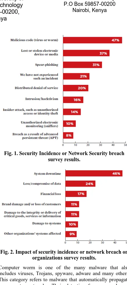
[image:1.595.318.536.158.645.2]The scope of this study is feature selection as a step in computer worm detection using machine learning approaches. Malware is any malicious software. According to [1], on average, a malware event occurs at a single organization once every three minutes. The nature of these incidents has changed from broad, scattershot assaults to very targeted attacks, with persistent adversaries causing significant damage to organizations and individuals alike. Figure 1 and Figure 2 show types of security incidents experienced by organizations and what their impact has been in the year 2013. It is evident that computer viruses and worms present a huge problem.
Fig. 1. Security Incidence or Network Security breach survey results.
Fig. 2. Impact of security incidence or network breach on organizations survey results.
Computer worm is one of the many malware that also includes viruses, Trojans, spyware, adware and many others. This category refers to malware that automatically propagate in computer networks. Their detection faces a number of challenges that include
The goal of feature selection is to identify the subset of differentially expressed fields of network packet headers that are potentially relevant for distinguishing the sample classes.
Feature selection is defined as a process that selects a subset of original features [13] [7] with the optimality of a feature being measured by an evaluation criterion [13]. [12], [5] add that the process selects relevant features while removing irrelevant, redundant and noisy features from data. For the section of the discussion that follows, the definition adopted is that feature selection is a process that selects a subset of original features while removing irrelevant, redundant and noisy features from data with the optimality of a feature measured by an evaluation function.
Feature selection has a number of benefits. These include facilitating data visualization and understanding, reducing measurement and storage requirements, reducing training and utilization times, defying the curse of dimensionality and improving prediction performance and avoiding overfitting. ([10, 12, 16]). [6] explain overfitting as using irrelevant variables for new data leading to poor generalization.
Feature selection methods can be categorized into filter methods, wrapper methods and embedded methods. These methods are discussed as follows:
[image:2.595.316.553.319.515.2]Filter methods select features using a preprocessing step. They totally ignore the effects of the selected feature subset on the performance of the induction algorithm. Figure 3 shows filter method.
Fig. 3. Filter Approach
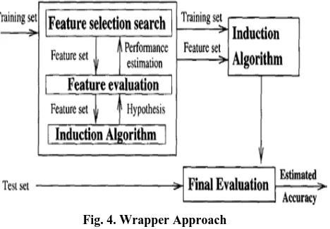
Another category of methods used for feature selection is wrappers method. These use the predictive performance of a given learning machine to assess the relative usefulness of subsets of variables [15, 10]. The induction algorithm is run on the dataset with different sets of features removed from the data. The feature subset with the highest evaluation is chosen as the final set on which to run the induction algorithm. Figure 4 shows wrapper approach.
Fig. 4. Wrapper Approach
[image:2.595.54.277.379.422.2]The last category of methods for feature selection are embedded. These incorporate feature selection as part of the training process
[10, 15].
2.
RELATED LITERATURE
A number of particular implementations for the methods discussed above are here reviewed.
A tree regularization framework which enables many tree models to perform feature selection efficiently has been proposed by [8]. The key idea is to penalize selecting a new feature for splitting when its gain is similar to the features used in previous splits. If gain(xj) is the evaluation measure calculated for feature xj. If the split feature at a tree node is selected by maximizing gain(xj) and F is the feature set used in previous splits in a tree model, the idea of the tree regularization framework is to avoid selecting a new feature xi, unless gain(xi) is substantially larger than maxi(gain(xi)) for xi C F. To achieve this goal, a penalty to gain(xj) is considered for xi C F. A new measure is calculated as
[image:2.595.57.291.517.680.2]Where ϒ C [0,1] and is the coefficient. The F from a built regularized tree model is expected to contain a set of informative but non redundant features.
Figure 5 shows tree based feature selection
Fig. 5. Regularized tree feature selection
[17] propose a two-stage method to implement feature selection. In the first stage, Information Gain (IG), a filter method was used to select informative genes. Features were sorted in accordance with their information gain values. A threshold for the results was established and features filtered out. In the second stage, Genetic Algorithm (GA), a wrapper method, was implemented. [9] presents a filter approach. The feature selection picks features which maximize their mutual information with the class to predict, conditionally to the response of any features already picked. A feature X0 is good only if I(Y ;X ̍ X) is large for every X already picked. This means that X is good only if it carries information about Y and if this information has not been caught by any of the X already picked.
worm behaviors that are useful for their classification and can be found in the packet headers.
3.
METHODS
3.1 Data set and tools.
The datasets used for the experiments were obtained from the University of San Diego California Center for Applied Data Analysis (USCD CAIDA). The center operates a network telescope that consists of a globally rooted /8 network that monitors large segmentsof lightly used address space. There is little legitimate traffic in this address space hence it provides a monitoring point for anomalous traffic that represents almost 1/256th of all IPv4 destinationaddresses on the Internet.
Two sets of datasets were requested and obtained from this telescope. The first is the Three days of Conficker Dataset ([2])containing data for three days between November2008 and January 2009 during which Conficker worm attack ([4]) was active. This dataset contains 68 compressed packet capture(pcap) files each containing one hour of traces. The pcap files only contain packet headers with the payload having been removed to preserve privacy. The destination IP addresses have also beenmasked for the same reason.
The other dataset is the Two Daysin November 2008 dataset ([3]) with traces for 12 and 19 November 2008, containing two typical days of background radiation just prior to the detection of Conficker which has been used to differentiate between Conficker-infected traffic and clean traffic.
The datasets were processed using the CAIDA Corsaro software suite ([11]), a software suite for performing large-scale analysis of trace data. The raw pcap datasets were aggregated into the Flow- Tuple format. This format retains only selected fields from captured packets instead of the whole packet, enabling a more efficient data storage, processing, and analysis. The 8 fields are source IP address, destination IP address, source port, destination port, protocol, Time To Live (TTL), TCP flags, IP length. An additional field, value, indicates the number of packets in the interval whose header fields match this FlowTuple key.
[image:3.595.310.548.78.312.2]The instances in the Three Days of Conficker dataset have been further filtered to retain only instances that have a high likelihood of being attributable to Conficker worm attack of the year 2008. [4] focuses on Confickers TCP scanning behavior (searching for victims to exploit) and indicates that it engages in three types of observable network scanning via TCP port 445 or 139 (where the vulnerable Microsoft software Windows Server Service runs) for additional victims. The vulnerability allowed attackers to execute arbitrary code via a crafted RPC request that triggers a buffer overflow. These are local network scanning where Conficker determines the broadcast domain from network interface settings, scans hosts nearby other infected hosts and random scanning. Other distinguishing characteristics of this worm included TTL within reasonable distance from Windows default TTL of 128, incremental source port, incremental source port in the Windows default range of 1024-5000, 2 or 1 TCP SYN packets per connection attempt instead of the usual 3 TCP SYN packets per connection attempt due to TCPs retransmit behavior. 100 instances of the Confiker dataset flowtuples were chosen randomly. These were then filtered out into 294 flowtuples using the distinguishing characteristics of Confiker worm attacks. Table 1 shows 5 instances of the Confiker dataset after this processing.
Table 1. Instances of confiker after processing
src_ip dst_ip sr cp d st p pr ot tt l tc pf i p l v a l cls 119.95.1 19.105 0.26.2 2.11 27 89 4 4 5
6 1 0 9 0x 02 4 8
2 mali ciou s 1190.55. 158.216 0.121. 102.55 46 95 4 4 5
6 1 0 9 0x 02 4 8
2 mali ciou s 231.39.2 38.24 0.126. 9.63 25 56 4 4 5
6 1 0 5 0x 02 4 8
2 mali ciou s 201.98.1 .3 0.98.8 0.118 45 86 4 4 5
6 1 0 4 0x 02 4 8
2 mali ciou s 190.51.7 8.219 0.128. 5.64 40 72 4 4 5
6 1 0 6 0x 02 4 8
2 mali ciou s
The datasets were then marked malicious adding another
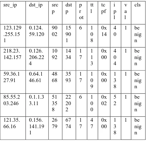
column to the dataframe. Similarly, random instances were chosen from the Two Days in November 2008 dataset. These represented, as indicated in Chapter 3 background traffic before the onset of the confiker worm. An equal number of instances were picked at random, hence 294 instances. These were then marked benign. Table 2 shows a sample of these.Table 2. Instances of benign traffic
src_ip dst_ip src p dst p p r ot tt l tc pf i p l v a l cls 123.129 .255.15 1 0.124. 59.120 90 02 15 90 1
6 1 0 8 0x 14 4 0
1 be nig n 218.23. 142.157 0.126. 206.22 4 10 92 14 34 1 7 1 1 3 0x 00 4 0 4
1 be nig n 59.36.1 27.91 0.64.1 46.61 48 68 35 93 1 7 1 0 9 0x 00 1 3 8
1 be nig n 85.55.2 03.246 0.1.1.3 3.11 51 35 8 22 20 2
6 1 0 0 0x 02 5 2
1 be nig n 121.35. 66.16 0.156. 141.19 1 26 79 67 74 1 7 4 7 0x 00 1 3 8
1 be nig n
[image:3.595.310.549.415.646.2]Table 3. Worms and Benign traffic
src_ip Src_ port
dst p
p or t
tt l
tc pf
ip l
v a l
cls ipc
82.230. 81.157
628 26
35 26 8
6 1 0 3
0x 14
4 0
2 ben ign
Fran ce
91.42.8 7.117
555 69
49 00 0
6 4 1
0x 00
4 0 4
3 ben ign
Ger man y
219.23. 56.163
494 3
13 5
6 9 6
0x 00
1 3 8
1 ben ign
Japa n
218.75. 199.50
199 1
14 34
1 7
1 1 1
0x 02
5 2
1 ben ign
Chin a
200.112 .144.28
430 1
44 5
6 1 0 4
0x 00
1 3 8
2 ben ign
Arge ntina
An additional column to hold a value 1 if the source port was similar to the destination port and a value 0 otherwise was created. Same source and destination ports may be indicative of worm activity since worms attack similar services in machines that are vulnerable. Worms attack most commonly used services. Ports in the range 0 to 1024, otherwise known as well-known ports, are more likely to be candidate for worm traffic. A column was further added to take care of this. This was done for both source port and destination port. Worm attacks are also likely to originate from hosts that are rarely initiate traffic in usual communications. A column was added to capture this situation. Categorical columns were then encoded using dummy variables. The total number of columns after the transformations is then 91 while the number of instances (rows) is 588. These is what is then used for the feature selection experiments. Python and the library scikit learn [14] has been used for the feature selection experiments.
3.2 Support Vector Machine(SVM)
SVM theory has been developed gradually from Linear SVCs to hyperplane classifiers, that is, SVMs can efficiently perform nonlinear classification by using a kernel function, implicitly wrapping their inputs into high-dimensional feature spaces by selecting an appropriate kernel function. Furthermore, a favorable classification result is achieved using a hyperplane that has the largest distance from the nearest training data point of any class. Given a training dataset D(xi; yi), where xi denotes n observations of malware signatures, xi Є R
N
, i = 1,…,N; and yi is the corresponding class label whose value is either 1 or -1, that is, malicious or benign, indicating the class to which the point xi belongs, yi Є 1,-1, assigned to each observation xi. Each behavioral signature xi is of dimension d corresponding to the number of proportional variables.
A typical clustering problem is identifying the maximum margin of a hyperplane that divides the points exhibiting yi = 1 from those exhibiting yi = -1. Any hyperplane can be written as the set of points, x, satisfying the following formula: w:xi+b = 0
∀
i where . denotes the dot product and wdenotes the normal vector of the hyperplane. The parameter
𝑏
𝐼𝐼𝑤𝐼𝐼etermines the offset of a hyperplane from the origin along
the normal vector w. Generally, a decision function D(x) is defined for clustering as D(x) = w:x + b A traditional linear SVM has a key drawback, that is, assuming that the training data are linearly separable, a [?] suggested a novel approach to generate nonlinear classifiers by applying a kernel function to maximum-margin hyperplanes. The nonlinear algorithm is formally similar to the linear SVM, except that each dot product is replace by a kernel function. The effectiveness of the SVM depends on the selection of a kernel and the parameters of the kernel. Kernels include linear, polynomial, radial basis function, sigmoid among others.
4.
EXPERIMENTAL RESULTS
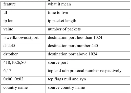
The meaning of the above identified feature set items are as presented in Table 4.
Table 4. Feature Meaning
feature what it mean
ttl time to live
ip len ip packet length
value number of packets
iswellknowndstport destination port less than 1024
dst445 destination port number 445
dstother destination port above 1024
418,1026,80 source port
6,17 tcp and udp protocal number respectively
0x00, 0x02 tcp flags null and syn
country name source country name
All low-variance features were removed by variance threshold technique. These are features which had similar values in 80 percent of the instances. These would not be useful for the classification experiments. The remaining features included time to live, ip packet lengths,the number of packets in the interval whose header fields matched a FlowTuple key, well known ports, the destination port 445 and port 1026, TCP and UDP protocol numbers, null and syn tcp flags and packet country of origin China.
[image:4.595.314.579.266.454.2]Fig. 6. Feature Correlation Heat Map
[image:5.595.316.543.120.314.2]Feature selection using these features and Linear SVC classifier yielded the confusion matrix shown in Figure 7.
Fig. 7. Feature Selection with Correlation Confusion Matrix
There were a number of misclassifications especially the False Negatives (instances that were malicious but were classified as benign). An accuracy of 0.91 was registered. The False Negatives were very few (Instances that were were not worms but were classified as worms). This is very encouraging. Univariate feature selection and Linear SVC gave a classification accuracy of 0.91 as well. The feature set was
[image:5.595.312.563.396.580.2]however slightly different with iplen scoring much higher than the rest. It is followed by ttl, iswellknowndstport,China and lastly value. The corresponding confusion matrix was as shown in Figure 8.
Fig. 8. Univariate Feature Selection Confusion Matrix
Again, a few misclassifications. Recursive Feature Elimination wrapper method picked the best features as iplen, value, iswellknowndstport and China. Classification accuracy improved to 0.92. The corresponding confusion matrix was as seen in Figure 9.
Fig. 9. Recursive Feature Selection Confusion Matrix
[image:5.595.54.286.429.662.2]Fig. 10. Feature Importance
As can be seen, iswellknowndstport, iplen, value, ttl and China were ranked in that order.
5.
DISCUSSIONS
The fields of network packet headers useful for the detection of computer worms included Time to Live, IP packet length, Wellknown ports and Source Country. It is instructive that computer worms target well known ports where popular services run for maximum impact and this explains why this feature is of importance for the classification. Conficker worm, for example, targets port 445 or 139 citepemile2009. The country likely to be the origin of the worm traffic was China. This is in line with the study by citefachkha2012, citefachkha2013 that also indicated Russia and China as the countries most likely to originate malicious darknet traffic. Packets coming from this country could be rated suspicious with a higher confidence value than those from other countries. IP packet length was also another useful feature for the detection. It is worth noting that worm packets are within particular ranges. The proposed two-stage method also improved feature selection. Other wrapper methods combined with Univariate feature selection methods could be investigated in future to improve the detection even further.
6.
CONCLUSIONS
This work investigated the features of computer worms useful for their classification using a number of feature selection methods. It was found out that iswellknowndstport, iplen, value, ttl and China were the most instructive features. This was in line with what literature has reported. These features of packet headers could be further investigated. The proposed feature selection methodology performed slightly better than univariate feature selection. The feature set used is small and so this methodology should be fast in implementation. Future work could investigate exploring other univariate feature selection schemes and other wrapper and embedded schemes. Also, the feature set could be expanded.
7.
REFERENCES
[1] The need for speed: 2013 incident response survey. Technical report.
[2] The caida ucsd network telescope ”three days of conficker”,1995(accessed February 3, 2014).
[3] The caida ucsd network telescope ’two days in november2008’ dataset, 1995(accessed February 3, 2014).
[4] Emile Aben. Conficker/conflicker/downadup as seenfrom the ucsd network telescope. Technical report,https://www.caida.org/research/security/ms08067c onficker.xml, 2009.
[5] Veronica Bolon, Noelia Sanchez, and Amparo Alonso. A reviewof feature selection methods on synthetic data. KnowledgeInformation Systems, 2013.
[6] Girish Chandrashekar and Ferat Sahin. A survey on featur selection methods. Computers and Electrical Engineering, 40(1):16–28, 2014.
[7] M Dash and H Liu. Feature selection for classification. Intelligent data analysis, 1997.
[8] Houtao Deng and G. Runger. Feature selection via regularized trees. In The 2012 International Joint Conference on Neural Networks (IJCNN), pages 1–8, June 2012.
[9] Franc¸ois Fleuret. Fast binary feature selection with conditional mutual information. Journal of Machine Learning Research, 5(Nov):1531–1555, 2004.
[10]Isabelle Guyon and Andre Elisseeff. An introduction to variable and feature selection. Journal of Machine Learning Research, pages 1157–1182, 2003.
[11]Alistair King. Corsaro, 2012
[12].Vipin Kumar and Sonajharia Minz. Feature selection a literature review. Smart Computing Review, 4(3), 2014.
[13]Huan Liu and Lei Yu. Toward integrating feature selection algorithms for classification and clustering. IEEE Transactions on Knowledge and Data Engineering, 17(4):491–502, April 2005
[14]F. Pedregosa, G. Varoquaux, A. Gramfort, V. Michel, B. Thirion, O. Grisel, M. Blondel, P. Prettenhofer, R. Weiss, V. Dubourg, J. Vanderplas, A. Passos, D. Cournapeau, M. Brucher, M. Perrot, and E. Duchesnay. Scikit-learn: Machine learning in Python. Journal of Machine Learning Research, 12:2825–2830, 2011. [15]Kohavi Ron and George John. Wrappers for feature
selection. Elsevier Artificial Intelligence, 97(1-2):273324, 1997.
[16]Vanaja S and Kumar Ramesh. Analysis of feature selection algorithms on classification a survey.
International Journal of Computer Applications, 90(17):29–35, 2014.