Robust H∞ Controller Design for the Nuclear Reactor Systems

15

Robust H∞ Controller Design for the Nuclear Reactor

Systems

Rehab M. Saeed

Nuclear Research Center

Egyptian Atomic Energy

Authority

Gamal M. El Bayoumi

Aerospace Engineering Dept.

Cairo University

Ibrahim E. Zeidan

Computers and Systems

Engineering Dept.

Zagazig University

ABSTRACT

As it is important to improve the response of the nuclear reactor power system, many approaches tried to find the best way to design the suitable robust controller .This paper introduces the solution of H∞ control problem of the nuclear

reactor systems as a robust controller that achieves both the robustness and performance improvement.

Keywords

H∞, Robust control, nuclear reactor systems, robustness

1.

INTRODUCTION

The first mission of the design of the H∞controller is to make the system insensitive towards the externals disturbances .this means that it is important to make the output independent of the external disturbance as possible [1].

The solution of the H∞ problem can be formulated in many

ways [2], one is the Glover-Doyle algorithm which is the classic formulation as it achieves the basic mixed performance and robustness objectives through solving a family of stabilizing controllers such that 𝐹𝑙(𝑃, 𝐾) ≤ 𝛾

Where

P(s) represents the plant nominal transfer function, K(s) represents feedback controller and 𝛾 is the H∞ norm.

Another techniques are used for the design of the H∞

controllers such as two transfer function method and three transfer function method [2].

The properties of designing a controller using H∞ method can

be summarized as that the stabilizing feedback low u(s) =K(s) y(s) minimizes the norm of the closed loop transfer function, and it is suitable for the weighted mixed sensitivity problem where H∞ controller always cancels the stable poles

of the plant with its transmission zeroes so the unstable poles of the plant inside the specified bandwidth will be shifted to its mirror image once a H∞ feedback loop is closed, another

property is that using suitable weighting functions will allow very precise frequency domain loop shaping [3].

Mixed weight H-infinity controllers [4] will provide a closed loop response of the system according to the design specifications such as model uncertainty, disturbance attenuation at high frequencies,….etc. The H∞ controllers are

of high order this may lead to large control requirements, also additional frequency dependent weights are augmented to the system.

The selection of the additional frequency dependent weights depends on what stability and performance design specifications are required to be shown [5].

Conventionally, H∞ controller employs two transfer functions

which divide a complex control problem into two separate sections, one deals with stability and the other deals with the performance. So the objective of designing H∞ controller is to

find a controller K, which based on the information v, generates a control signal u, which compensates the influence of w on z and minimizes the closed loop norm w to z.

The paper is organized as follow, section 2 represents the nuclear reactor model (actual and nominal plants).Section3 introduce the H∞ optimal control while the simulation results

are represented in section 4 and the conclusion is introduced in section 5.

2.

NUCLEAR REACTOR MODELING

The model used in this paper is the nominal Pressurized Water Reactor model (PWR-type) TMI nuclear power plant reactor and its kinetic equation with one delayed neutron group and temperature feedback.

The actual system equations can be summarized in the following equations [6]:

dn dt =

δρ−β

∧ n −λc (1) dc

dt=

β

∧n −λc (2)

Where,

n ≡ neutron density (n

cm 3

)

c ≡ neutron precursor density atom

cm3

λ≡ effective precursor radioactive decay constant s−1

∧≡ effective prompt neutron lifetime(s) β≡ fraction of delayed fission neutrons

k ≡ keff≡ effective neutron multiplication factor

δρ≡k−1_k ≡ reactivity (Since k≈1.000,δρ ≈k-1 ; at steady state k=1 , δρ= 0)

For computational purposes the normalized versions of equations (1) and (2) will be used so the normalized equations will be as follow:

dnr

dt =

δρ−β

∧ nr+

β

∧cr (3) dcr

dt =λnr−λcr (4)

n0≡ initial equilibrium steady − state neutron density,

16

𝑛𝑟≡ 𝑛/𝑛0, neutron density relative to equilibrium density

𝑐𝑟≡ 𝑐/𝑐0, precursor density relative to initial equilibrium

density

As the reactor temperatures vary as a function of power generated and heat transfer and it affects the reaction chain so it has to be included in the normalized point-kinetic equations for accurate calculation of the output power ( nr).

Reactor temperatures can be expressed as following,

dTf

dt = ff P0a

μc

nr−

Ω μf

Tf+

Ω

2μf

Tl+

Ω

2μf

Te (5) dTl

dt = (1−ff)P0a

μ_c nr+

Ω μ_cTf−

2M+Ω

2μ_c Tl+ 2M−Ω

2μ_c Te, (6) dδρr

dt = GrZr (7)

δρ=δρ_r+αf Tf− Tf0 +

αc(Tl−Tl0)

2 +

αc(Te−Te 0)

2 (8)

The described model has five states which appear in the nominal model. These Five states are the relative reactor power (nr), the relative precursor density (cr), the average fuel

temperature Tf, the average coolant temperature leaving the

reactor Tl and the reactivity 𝛿𝜌𝑟 respectively. The model is

nonlinear because total reactivity 𝛿𝜌 which is composed of the rod reactivity 𝛿𝜌r and temperature feedback reactivity

from equation (8) multiplies the reactor power state to determine the reactor power rate change [6].

The linearized system can be represented by the following state space equations,

x = Ax + Bu ,y = Cx + Du (9)

Where,

x =

δnr

δcr

δTf

δTc

δρ_r

, y = δnr , and u = zr

And

A =

−βν β ν nr0

αf

ν nr0 αc

2ν

nr 0

ν

λ –λ 0 0 0

ffP0a

μf

0 −_μΩ

f

₂Ω_μ

f

0

1−ff P0a

μc

0 _μΩ

c

− (2M +Ω)/2μ_c 0 0 0 0 0 0

B = 0 0 0 0 Gr

, C = 1 0 0 0 0 and D = 0

δρ_r≡ Control rod reactivity,

δρ ≡𝛿𝜌𝑟 for a system without temperature feedback,

zr ≡ Control rod speed in units of fraction of core length per

second,

Gr≡ The reactivity worth of the control rod per unit length.

With zr in units of fraction of core length per second and Gr is

the total worth of the rod.

The simulation has been done by applying the controller to the nonlinear system while the linearized reactor model is used to design the suitable controller.

3.

H

CONTROLLER DESIGN

Figure 1 Design of H infinity controller

The model in figure (1) consists of P(s) and K(s), where P(s)

has the multi inputs of disturbances vector w that contains the system uncertainty and the measurement noise plus the control input u while the output is y and z.

As H∞ controller design depends on solving two Riccati

equations one for the state feedback control and the second for the estimation problem so the problem can be similar to Linear Quadratic Gaussian control (LQG). However there is a difference between H∞ control and LQG control as the

standard H∞ optimal control problem is concerned with

constructing a dynamic feedback controller u=K(s)y to minimize the H∞ norm of the transfer function from w to z,

[8].

Assume the state space equations of the system are in the following form

x = Ax + B1w + B2u (10)

z = C1x + D11w + D12u (11)

y = C2x + D21w + D22u (12)

And can be packed in G(s) as one matrix represents the system parameters where,

G s =

A B1 B2

C1 D11 D12

C2 D21 D22

(13)

Some important assumptions have to be done as [8]:

 The pair (A, B2) are stabilizable and the pair (C2,A) are

detectable.

 D11=0 and D22=0 in order to simplify the solution.

 Dimension (x), dimension (w)=m1 while dimension

(u)=m2, also dimension (z)=p1 and dimension (y)=p2,

then the rank of D12=m2 and the rank of D21=p2. These

assumptions will ensure that the controllers are proper

 RankA − jwI B2

C1 D12 = n + m2 for all frequencies.

 Rank A − jwI B1

17 Now the new system will be describes as:

G s =

A B1 B2

C1 0 D12

C2 D21 0

(14)

The solution of this equation (equ 14) requires solving two Riccati equations one for the controller and the other for the observer and the control law is given by

u = −Kcx (15)

And the state estimator equation is

x = Ax + B2u + B1w + Z∞Ke(y − y ) (16)

Where

w =γ−2_B 1TX∞x

y = C2x +γ−2D21B1TX∞x

And the controller gain Kc is

Kc= D12(B2TX∞+ D12T C1

Where,

D12= (D12TD12)−1

And the estimator gain is Z∞Ke instead of Ke where,

Ke= y∞C2T+ B1D21T )D21, D21= (D21D21T )−1 , Z∞=

(I −γ−2_Y

∞X∞)−1 and the terms X∞ and

Y∞ are the solution of the controller and estimator Riccati

equations,

X∞= Ric A − B2D12D12

T _C

1 −γ−2B1B1T− B2D12

−C 1TC 1 −(A − B2D12D12T)C1

(17)

Y∞= Ric (A − B1D21

T _D

21C2)T −γ−2C1TC1− C2TD21C2

−B1B1T −(A − B1D21T D21)C2

(18)

With

B1= B1(I − D21D21D21T )and C 1= B1(I − D12D12D12T)

The above calculations are not easy to be done by hand but it is done using the Matlab subroutines.

When the H∞ optimal control technique is applied to a plant

an additional frequency dependent weights are to be augmented in the plant and these weights are selected to show particular stability and performance specifications.

The problem now becomes a mixed weight H-infinity controller design which provides a closed loop response of the system.

The added weight functions are Ws and Wt, and they have to

be specified to meet the system specifications, where Ws is the

performance weighting function which limits the magnitude of S the sensitivity function and Wt is the robustness

weighting function to limit the magnitude of T the complementary sensitivity function.

4.

SIMULATION AND RESULTS

The following values represent the parameters of the TMI pressurized water Reactor [6]

According to the assumptions taken into account the following parameters are used for the simulation using Matlab Toolbox [10].

D11= 0 0_{0 0} and D22= 0,

D12= 0₁ and D21= 0 −1 ,

B1= 0₀0₀0₀0₀1₀ T

, which represents the disturbance acts on

the system,

C1= 1₀0₀₀00₀0₀ and C2= −1 0 0 0 0

The normalized system transfer function is:

Gs = 100s3+173.6s2+52.82s+4.085

s5_+66.74s4_+151.8s3_+90.17s2_+7.8845s

And the designed controller K has the following form

1:Ks =-369.3s

4_-5.395e04s3_-9.278e04s2_{-2.824e04s-2185}

s5_+66.75s4_+152.5s3_+91.83s2_{+8.845s+0.08435}

2:Ks =-2.789e04s4-1.861e06s3-4.161e06s2-2.411e06s-2.116e05

s5_+66.75s4_+152.5s3_+91.83s2_{+8.845s+0.08435}

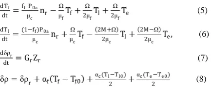
And by applying the designed controller to the augmented plant the following results are obtained

Figure 2 Relative reactor power

0 10 20 30 40 50 60 70 80 90 100

0.1 0.2 0.3 0.4 0.5 0.6 0.7 0.8 0.9 1

relative reactor power

Time in seconds

re

la

ti

ve

r

e

a

c

tor

pow

e

r

nr

β =0.0065 λ= 0.125 s-1

∧=0.0001 s ff =0.98

Gr=0.01 total rod reactivity Te =290 C

P0a=2500 MW μc =70.5 MW s/C

μf =26.3 MWs/c M=92.8 MW/C

Ω =6.53 MW/C αf =-0.00005 reactivity /C

18

Figure 3 Relative precursor density

Figure 4 Fuel temperature

Figure 5 Coolant temperature

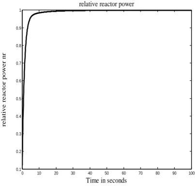
Figure 6 Relative reactivity

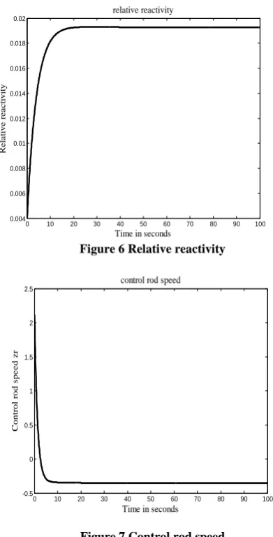
Figure 7 Control rod speed

5.

CONCLUSION

Simulation results show that the time response of the output power and the control input as well. From these results it is observable that the system reaches its steady state in about 60 seconds and the maximum control rod speed does not exceed 2cm/sec which is a constraint for the control rod speed [9]. Also it is noticeable from the results that H-infinity controller achieves both robustness and good performance as it rejects the disturbances effectively.

Also the results show that the suggested control technique improves the fuel and temperature responses and the responses do not suffer from any overshoots.

Comparing the obtained results in this paper by the results obtained in H2 controller of the nuclear reactor [11] paper one can find that both of the techniques satisfy sufficient control requirements of the nuclear reactor.

It is recommended to apply the same technique to the reactor in the case of changing the power level by increasing or decreasing and also in case of low power (10%) to achieve a good control of the system in these cases.

0 10 20 30 40 50 60 70 80 90 100

0.65 0.7 0.75 0.8 0.85 0.9 0.95 1

relative precursor denisty

Time in seconds

R

e

la

ti

ve

pr

e

c

ur

sor

de

ns

it

y

0 10 20 30 40 50 60 70 80 90 100

400 450 500 550 600 650 700

Fuel temperature

Time in seconds

F

ue

l

te

m

pe

ra

tur

e

T

f

0 10 20 30 40 50 60 70 80 90 100

302 304 306 308 310 312 314 316 318

coolant temperature

Time in seconds

C

ool

a

nt

T

e

m

pe

ra

tur

e

T

l

0 10 20 30 40 50 60 70 80 90 100

0.004 0.006 0.008 0.01 0.012 0.014 0.016 0.018 0.02

relative reactivity

Time in seconds

R

e

la

ti

ve

r

e

a

c

ti

vi

ty

0 10 20 30 40 50 60 70 80 90 100

-0.5 0 0.5 1 1.5 2 2.5

control rod speed

Time in seconds

C

ont

rol

r

od

s

pe

e

d

z

19

6.

REFERENCES

[1] J. Treunicht, May 15,2007, “H∞ control”

[2] Ian R.Petersen,Valery A.Ugrinovski and Andrey v.Savkin,2000, “Robust Control design using H∞

methods”.

[3] Gerald a.Hartley,master thesis 1990,”Robust control design using H2 and H∞ methods”

[4] Ankit Bansal,Veena Sharma,”Design and Analysis of Robust H-infinity Controller”.

[5] Zames G,1981, “feedback of optimal sensitivity Model reference transformation ,Multiplicative semi-norms and approximate Inverse”, IEEE Trans, Ac vol Ac-26.

[6] Robert M.Edwards, Kwange Y.Lee and Asok Ray ,1991 .Robust optimal control of nuclear reactors and power plants, University Park, Pennsylvania.

[7] Doyle J. C., Glover K., Khargonekar P. P and Francis B. A., 1988, “state space solution to standard H2 and H∞

control problems”, American control conference, Atlanta.

[8] Zhou K. and Khargonerkar P. P , 1988, “An algebraic Riccati Equation Approach to H∞ optimization” systems

and control letters.

[9] Yoon-Joon lee and Jung-In Choi, 1997, “Robust Controller Design for the Nuclear Reactor Power Control System”, Journal of the Korean Nuclear Society.

[10] Richard Y. Chiang and Michael G. Safono, 1997,”Matlab Robust Control Toolbox”.

[11] Rehab M.Saeed and Gamal.M. El-bayoumi, 2017, “Robust H2 control of the nuclear reactor”,IJCA.