An Experimental Method to Determine the Cut Off Frequency of an Acoustical Free Field in a Non Ideal Environment

ISSN Online: 2162-5794 ISSN Print: 2162-5786

DOI: 10.4236/oja.2018.81001 Mar. 31, 2018 1 Open Journal of Acoustics

An Experimental Method to Determine the

Cut-Off Frequency of an Acoustical Free

Field in a Non-Ideal Environment

Mohammad Al Zubi

Mechanical Engineering Department, Tafila Technical University, Tafilah, Jordan

Abstract

The availability of ideal conditions like anechoic chamber to characterize some sound parameters, like sound intensity and sound power necessities the determination of free field and cut off frequency measurements. In this article, full experiment was executed at Wayne State University (Detroit-Michigan), to determine the cut off frequency in all directions; the obtained results showed that the free field can be determined for a specified space. So other tests can take place in this space avoiding regions where reflections and consequently noise can be found. Upon these results tests related to noise abatement in ve-hicles can be done in such environment.

Keywords

Acoustics, Cut-Off Frequency, Sound Fields, Noise

1. Introduction

Sound can be defined as any pressure variation which can be detected by human ear. It is an important part of our life. It provides enjoy such as listening to a singing bird. It enables us to communicate with other people [1]. On the other hand, sound may be unwanted, in the case it is called noise, either because of its effect on humans or malfunction of physical equipment, or its interference with the perception or detection of other sounds so abatement of this phenomena becomes necessary [2][3].

Sound propagates at different speeds depending upon media, for example the speed of sound in air is about 340 m/s, whereas in water it reaches around 1500 m/s [4].

The sound field is a region where there is sound. It is classified according to

How to cite this paper: Al Zubi, M. (2018) An Experimental Method to Determine the Cut-Off Frequency of an Acoustical Free Field in a Non-Ideal Environment. Open Journal of Acoustics, 8, 1-11.

https://doi.org/10.4236/oja.2018.81001

Received: March 7, 2018 Accepted: March 28, 2018 Published: March 31, 2018

Copyright © 2018 by author and Scientific Research Publishing Inc. This work is licensed under the Creative Commons Attribution International License (CC BY 4.0).

DOI: 10.4236/oja.2018.81001 2 Open Journal of Acoustics

the manner and the environment in which the sound waves travel.

1) Free field describes sound propagation in idealized free space where there is no reflections [5]. This condition holds in an anechoic room where all the sound striking the walls is absorbed. Free field is characterized by a 6 dB drop in sound pressure level and intensity level each time the distance from the source is doubled [6].

2) Near field of a source is the region close to a source [7]. In this region, the sound field does not decrease by 6 dB each time the distance from the source is increased [8]. The near field is limited to a distance from the source equal to about a wavelength of sound or equal to three times the largest dimension of the sound source (whichever is the larger) [9].

3) Far field of a source begins where the near field ends and extends to infin-ity [10].

So it is important to find an experimental method to find the different fields of sound in non-ideal conditions depending upon cut off frequency, when this is achieved, it is easy to implement testing of vehicles related to NVH issues.

2. Basic Theory

Sound waves are characterized by the amplitude of pressure changes, which

can be described by the root-mean-square (RMS) amplitude, prms, and is

ex-pressed in Pascal (Pa). Root-mean-square means that the instantaneous sound pressures (which can be positive or negative) are squared, averaged and the square root of the average is taken as shown in Equation (1) [11], and Figure 1

respectively.

rms 0.707 max

p = p (1)

Noise is usually composed of many frequencies combined together, the wave-length (λ), which is the distance travelled by the pressure wave during one cycle, the frequency (f), which is the number of cycles per second, and is expressed in Hertz (Hz) are related togother through the following equation [12]:

c= fλ (2)

DOI: 10.4236/oja.2018.81001 3 Open Journal of Acoustics

where (c) is the speed of sound, in air it is 343 m/s, at 20˚C and 1 atmosphere pressure [13].

The range of sound pressures that can be heard by the human ear is very large. The minimum acoustic pressure audible to the young human ear in good health, is approximately 20 × 10−6 _{Pa, the minimum audible level occurs at about 4000}

Hz [14]. A linear scale based on the square of the sound pressure would require 1013 _{unit divisions to cover the range of human experience [15]; a scale suitable}

for expressing the square of the sound pressure in units best matched to subjec-tive response is logarithmic rather than linear. Thus the Bel [16], was introduced which is the logarithm of the ratio of two quantities, one of which is a reference quantity. The level of sound pressure p is then said to be Lp decibels (dB) greater

or less than a reference sound pressure pref (20 μPa) according to the following

equation [3]:

2

rms rms

10 2 10 10 rms 10 ref

ref ref

10 log P 20 log P 20 log 20 log

Lp P P

P P

= = = − ₍₃₎

3. Experiment Objectives, Setup and Procedure

The main objective of the experiment is to characterize a sound field, to find the cut off frequency for the free field of the source in each direction, so the suitable regions to take measurements in the space for future work will be known, like a case where the anechoic chamber is not available.

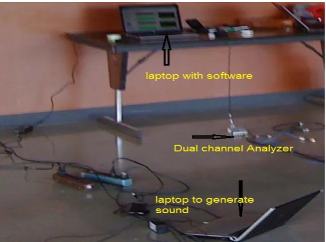
The major components used to execute the experiment are Bruel and Kjaer (B&K) dual channel signal analyzer Type 2032 [17], speaker, power amplifier, and signal generator, the detailed equipment are:

1) Sound source generated from a laptop then emitted through a loud speaker, it should be mentioned here that the speaker cover was removed to get sound free on any obstacles.

2) A space to characterize the free field for that space, a large room in the en-gineering building at Wayne State University was chosen, this room is near Warren road (noise source) and have two glass walls from the west and the south.

3) Two Bruel & Kjaer microphones, to measure the sound pressure level at many consecutive points drawn on the base of the room, those two microphones are connected to two channel analyzer for amplification, then the signal is sent to another laptop in which the software (LabVIEW) from national instruments was installed to do the calculations and get the results.

4) Different connections to connect the hardware parts

5) A calibrator to calibrate the microphones before stating the measurements according to standards, this calibrator is a piston phone B&K type 4220, Serial No. 704798.

Figure 2 shows the sound source, points drawn on the ground, and the mi-crophones, mic2 was near the source (leads mic1).

DOI: 10.4236/oja.2018.81001 4 Open Journal of Acoustics Figure 2. Experimental setup including, sound source, microphones, and points on ground.

Figure 3. Other part of the experimental setup including the sound generator laptop, the sound analyzer and the data acquisition system.

data, also the dual channel analyzer appears.

Figure 4 shows a picture for the room under test in which chairs, air conditioning unit, glass walls, can be seen, all these things contribute in adding noise to the measurements, this is why the environment is not ideal.

DOI: 10.4236/oja.2018.81001 5 Open Journal of Acoustics Figure 4. Noise sources in the room under test including the street, and the air conditioning unit.

that reference point, 9 points were marked in each direction (N, S, E, W), the distances from the source are (4, 8, 12, 16, 24, 32, 48, 64, 80, 96) inch, these points were selected because the experiment should be executed as far from glass walls as possible to avoid reflection. 2 stands were used to mark the same points in the 45˚ for each direction, finally a direction upward was selected with the same distances, so a hemisphere space shape was obtained for the measure-ments.

DOI: 10.4236/oja.2018.81001 6 Open Journal of Acoustics

exported to an excel sheet in which SPL in each direction for the mentioned dis-tances is analyzed for the selected frequency range.

4. Results and Discussion

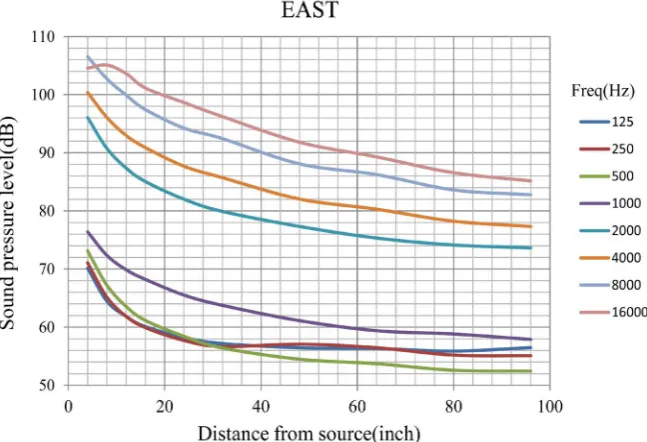
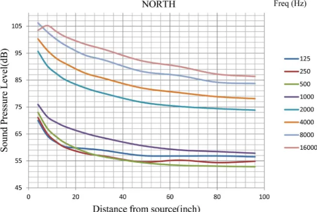
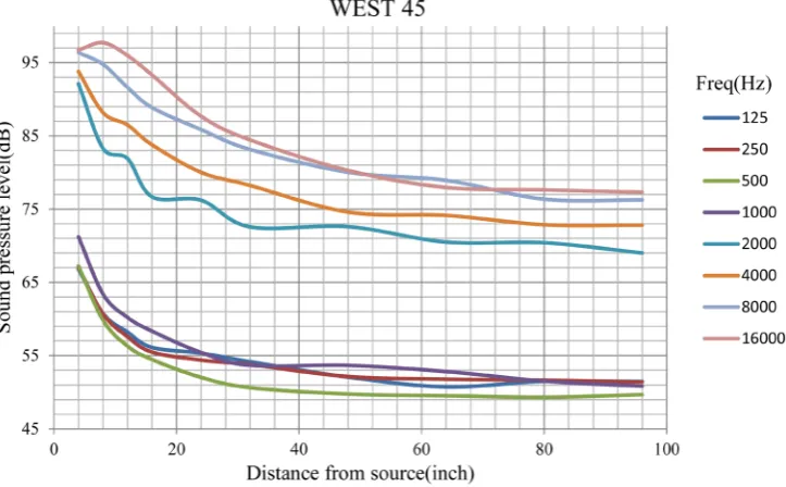
The excel files exported from the software have three readings, the frequency, the sound pressure level (SPL) for microphone 1, SPL for microphone 2, the data were taken for each direction and frequency, then the SPL versus the distance was drawn, from which a logarithmic curve fit was drawn to be able to see the dB drop which guide to a free field (5 - 6 dB drop between doubled distances). The charts show the SPL versus distance for each direction and for the frequency band from (125 Hz - 16 kHz).

It should be noticed here that the cut-off frequency is when the difference in SPL values between two spectra is less than 6 dB, in all figures the graphs show the relationship between sound pressure level versus distance from the source for a specified frequency rang.

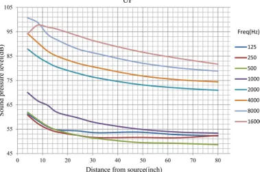
From the experimental results, the following was noticed for each direction: 1) In the east direction (Figure 5), the cut-off frequency was 2 kHz, on the other hand the free field covers the entire distance (4 - 96 inch) for the frequn-cies (8, 16) kHz, for the frequency 2 kHz, the ranges (8 - 16, 32 - 64 inch), and for the frequency 4 kHz, the ranges (16 - 32, 48 - 96 inch) are not a free field re-gions.

2) In the west direction (Figure 6) the cut-off frequency was 2 kHz, on the other hand the free field covers the entire distance (4 - 96 inch) for the entire frequncy band (2 - 16) kHz.

In this direction it was found that the cut-off frequency is 2 kHz, on the other

DOI: 10.4236/oja.2018.81001 7 Open Journal of Acoustics Figure 6. SPL as function of distance from source in the west direction at different fre-quncies.

Figure 7. SPL as function of distance from source in the north direction at different fre-quncies.

hand the free field covers the entire distance (4 - 96 inch) for the frequncies (2 - kHz, for the frequency 16 kHz, there is no free field regions.

3) In the north direction (Figure 7), the cut-off frequency was 2 kHz, on the other hand the free field covers the entire distance (4 - 96 inch) for the frequn-cies (2 - 8) kHz, for the frequency 16 kHz, there is no free field regions.

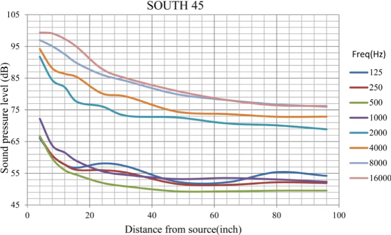
4) In the south direction (Figure 8), the cut-off frequency was 2 kHz, on the other hand the free field covers the entire distance (4 - 96 inch) for the entire frequncy band (2 - 16) kHz.

DOI: 10.4236/oja.2018.81001 8 Open Journal of Acoustics Figure 8. SPL as function of distance from source in the south direction at different frequncies.

Figure 9. SPL as function of distance from source in the west 45˚ direction at different frequncies.

frequency band frequncies (2 - 16) kHz.

6) In the north 45˚ direction (Figure 10), it was found that the cut-off fre-quency to be 2 kHz, on the other hand the free field covers the entire distance (4 - 96 inch) for the frequncies (2, 8, 16) kHz, for the frequency 4 kHz, the range (16 - 32 inch) is not a free field regions.

DOI: 10.4236/oja.2018.81001 9 Open Journal of Acoustics Figure 10. SPL as function of distance from source in the north 45˚ direction at different frequncies.

Figure 11. SPL as function of distance from source in the south 45˚ direction at different frequncies.

- 96 inch) for the frequncies (2 - 8) kHz, for the frequency 16 kHz, the ranges (16 - 32) is not a free field region.

DOI: 10.4236/oja.2018.81001 10 Open Journal of Acoustics Figure 12. SPL as function of distance from source in the up direction at different frequncies.

5. Conclusions

In this experiment, it was observed that the space where the experiment took place is a good acoustic space, this is clear from the SPL decay with distance; the reflections from the other sources affect the measurements with a low percen-tage. In this experiment, a human error may affect the measurements like speaking or walking while the mics capture the source sound, also the inclination of the source and the mics for 45˚ was not so accurate, the glass walls and the air con-ditioning unit add a noise to the measurements.

It was observed that the free field regions for the selected directions spread over a large area in the space which gives flexibility to do measurements.

In this experiment, characterization of a free field for a room in the real life was executed, how to determine the cutoff frequency in each direction, and the distances in space where the free field is found were clarified, this will give a guide to characterize other characteristics of this room like sound intensity and sound power. The determination of free field is an important issue in acoustics as it tells where the regions to avoid reflections are. Such an acoustical environ-ment can be used to test vehicles for noise abateenviron-ment aims in case the conditions for ideal test are not available.

References

[1] (1984) McGraw Hill Dictionary of Scientific Terms. 3rd Edition.

[2] Noise and Hearing Loss. NIH Consensus Development Conference Statement On-line 1990. 8, 1-24.

Engi-DOI: 10.4236/oja.2018.81001 11 Open Journal of Acoustics neering, University of Adelaide, Australia.

[4] Filippi, P. (Ed.) (1998) Acoustics: Basic Physics, Theory and Methods. [5] Smith, B.J., et al. (1996) Acoustics and Noise Control. 2nd Edition. [6] Microphone Handbook, PCB Piezotronics. www.pcb.com

[7] Onofrei, D. and Platt, E. (2018) On the Synthesis of Acoustic Sources with Control-lable near Fields. Wave Motion, 12-27.

[8] Spagnol, S., Tavazzi, E. and Avanzini, F. (2017) Distance Rendering and Perception of Nearby Virtual Sound Sources with a Near-Field Filter Model. Applied Acoustics, 115, 61-73. https://doi.org/10.1016/j.apacoust.2016.08.015

[9] Singh, A., Singh, R. and Lehana, P. (2016) Investigation of the Frequency Response of Shankha. IJAREEIE, 5.

[10] Bjørnø, L. (2017) Applied Underwater Acoustics. 85-184.

[11] Boashash, B. (2016) Time-Frequency Signal Analysis and Processing. 2nd Edition, Qatar University, Doha, 31-63.

[12] Alves, M. and Wav, E.C. (2016) Numerical Modelling of Wave Energy Converters, State-of-the-Art Techniques for Single Devices and Arrays, 11-30.

[13] Outcalt, S.L., Laesecke, A. and Fortin, T.J. (2010) Density and Speed of Sound Mea-surements of 1- and 2-Butanol. Journal of Molecular Liquids, 151, 50-59.

https://doi.org/10.1016/j.molliq.2009.11.002

[14] Hughes, P. and Ferrett, E. (2008) Introduction to Health and Safety in Construc-tion. 3rd Edition, 349-376. https://doi.org/10.1016/B978-1-85617-521-0.50024-9 [15] Kayode, A. and Ludwig, C. (2007) Applied Process Design for Chemical and

Petro-chemical Plants. 4th Edition, Process Safety and Pressure-Relieving Devices, 1, 575-770.

[16] Long, M. (2014) Architectural Acoustics. 2nd Edition, 39-79.