Lancaster University Management School
Working Paper 2018:3
Non-parametric dynamic pricing: a
non-adversarial robust optimization approach
Trivikram Dokka, Peter Jacko and Waseem Aslam
The Department of Management Science
Lancaster University Management School
Lancaster LA1 4YX
UK
© Trivikram Dokka, Peter Jacko and Waseem Aslam All rights reserved. Short sections of text, not to exceed two paragraphs, may be quoted without explicit permission,
provided that full acknowledgment is given.
Non-parametric dynamic pricing: a
non-adversarial robust optimization approach
∗
Trivikram Dokka
†Peter Jacko
Waseem Aslam
April 17, 2018
Abstract
We consider a single-product finite-horizon dynamic pricing problem where a seller seeks to maximize the expected revenue while learning how to dynamically ad-just the product price, without assuming a shape of the demand function. In this work we propose a non-adversarial robust optimization approach to the non-parametric dynamic pricing, where after the seller announces her price, and for a given level of her conservatism (captured by the statistical confidence level used for estimating the demand function), nature chooses a price distribution for the alternative product which minimizes the expected cost of the customer during that period. Our approach is thus different from the traditional robust optimization approach which assumes an adversarial setting, where nature chooses a price distribution for the alternative prod-uct which minimizes the expected revenue of the seller. We show that our algorithm is competitive, using simulated and real data, even without optimizing its parameters compared to the optimized version of the algorithm proposed in Besbes & Zeevi [Dy-namic pricing without knowing the demand function: Risk bounds and near-optimal algorithms. Operations Research, 57(6):1407–1420 (2009)]. We present a sensitivity analysis to show that further improvement in the performance is possible depending on the problem setting and on the decision maker’s level of conservatism.
Keywords: dynamic pricing; learning algorithm; robust optimization ∗Working paper
†Corresponding author, Department of Management Science, Lancaster University, UK,
1
Introduction
1.1
Motivation
Setting a price which generates highest revenue is an important problem faced by a seller of a product or service in many industries. The revenue maximizing price is generally not known to the seller and good (near-optimal) prices can often be learned by experi-menting with a number of different prices. However, it is important that the seller finds a good balance between revenue maximization and price experimentation, for two main reasons: (1) setting a sub-optimal price means a loss of potential revenue and (2) changing the price too frequently or too dramatically affects the customers’ perception of the prod-uct/service and/or may not even be feasible due to strategic or contractual constraints. As a result, sometimes it is better for the seller to settle, at least for a certain period of time, at a sub-optimal price instead of continuing price experimentation.
While this problem has been extensively studied in academic literature, the modelling assumptions are often unrealistic for practical use of the results. For instance, some els assume that the demand is deterministic and known as a function of price, other mod-els assume that the demand is stochastic and a distributional form of the demand function is known. In these cases, typically, no experimentation is needed as the optimal price can be derived theoretically or computed numerically using optimization and/or simulation techniques.
Price experimentation (leading to dynamic pricing) becomes important in more ad-vanced models, in which the demand is assumed to be stochastic, but the parameters of the distributional form of the demand function are not known. The seller learns these parameters by price experimentation and eventually fits the model at a sufficiently high precision to find an optimal price. However, in many situations such distributional as-sumptions may not be correct and both price experimentation and settling at an optimal price under wrong assumptions can be damaging to the seller’s revenue. In practice, the distributional form may not be known at all and it is desirable to address this prob-lem without making any assumptions on the distributional form of the demand function, which is the objective of this paper.
In [6], it is shown that a pricing policy like this is asymptotically optimal. Such a policy, however, is often not practical. Moreover, for many classes of products and services, the seller often faces restrictions such as price caps imposed by regulatory authorities, supply chains contracts, and/or seller’s marketing strategy. The reason this simple policy may not be feasible for such products is that seller is not free to change the price whenever she finds it desirable and to whatever price she finds it appropriate. For instance, if there is a cap on the price increase, the seller can end up in a situation with a very low price experimented at the end of the learning phase, being unable to set a higher price which she knows yields a significantly higher revenue. Another drawback of this policy is that it waits for price experimentation to finish with no attempt to use the information collected so far to adapt to in the rest of the learning phase.
In this paper, we propose anon-parametric dynamic pricingpolicy, which balances price experimentation with revenue maximization. It is non-parametric, because we do not assume a particular distributional form of the demand function; we only require the range of allowable prices to be known. We deploy a novel, non-adversarial robust optimization approach, which we extend and significantly generalize to a multi-period setting from the recently proposed static formulation in [9]. The approach is robust in two ways. First, in the sense that instead of using means, we use lower confidence bounds, which can be seen as having a risk-averse seller or a seller that takes a conservative stand when facing uncertainty in making estimations from data. It is also robust due to the formulation of a subroutine using a bilevel optimization problem, where the upper objective maximizes the expected revenue. The lower objective minimizes the expected cost of customer(s), which differentiates our approach from the traditional robust optimization approach in which the lower objective is adversarial (i.e., where nature chooses a price distribution for the alternative product which minimizes the expected revenue of the seller).
is also aforced exploration phase, which is designed to get out of the range of uninteresing prices (with very small demand) as quickly as possible.
There are several advantages of our proposed pricing policy with respect to the simple policy described above:
1. we allow the price to be adaptively changed whenever there is sufficient evidence from past data that a change is beneficial, i.e. without formally splitting the horizon into learning and earning phases;
2. we can incorporate price caps;
3. we can take into account seller’s level of risk-aversion.
1.2
Price Caps and Toll Roads
There is a long history of regulatory price controls used by governments in regulating the prices and usage of various important goods and products. Price controls were used by governments as early as the years following the French Revolution. Historically, there are numerous cases where governments around the world used some sort of price control in regulating markets for products ranging from oil, drugs, toll roads and property rents. One important reason for this is price control is seen by many as an easy political instru-ment to gain popularity. In many of these instances the private companies involved in selling products with price control have seen heavy losses. Naturally, many economists over the years reasoned against the use of price controls. Despite this, there are many instances where governments impose price controls.[1] notes that rate of return regula-tion is widely used in sectors like energy, telecommunicaregula-tions and transport. Under such regulation, firms selling products are not allowed to earn above a certain rate of return and price rises are capped. Authors also note that capped increase is usually linked to inflation index.
increase. A small or a capped increase on price should be promoted as it can be easier for customers to incorporate it in their spending patterns and gives the toll operators op-portunities to better manage their revenues. We quote from [7], “Careful contract negoti-ations can constrain maximum toll increases. The recent National Surface Transportation Policy and Revenue Commission report recommended capping toll rate increases at the level of the CPI, adjusted by productivity. Tolls on the Indiana Toll Road are scheduled by the Indiana legislature through June 2010. Thereafter, maximum annual increases for all vehicles are capped at the greater of2%, CPI, or per capita nominal growth in gross domestic product (GDP). Tolls on the Chicago Skyway are scheduled in the lease agree-ment until 2017, with maximum annual increases capped at the greater of2%, CPI, or per capita nominal GDP growth beyond 2017. Tolls on the Pocahontas Parkway in Richmond, Virginia, are specified until 2016, and annual increases are capped at the greater of2.8%, CPI, or per capita real GDP growth thereafter”. Our motivation for considering price control in such problems comes from the public sector, where a third party authority (like the government or a governmental regulation agency) can introduce price controls on the product provided by a revenue-maximizer involved in a public-private partnership or a similar scheme.
With restrictions like price caps seller is very constrained in price experimentation. Price caps require to set the tolls as robustly as possible to avoid any need for a price hike.
1.3
Related Literature on Dynamic Pricing
The dynamic pricing problem (DPP), in which a seller dynamically varies the price of a product with the objective of maximizing the expected revenue over a finite time hori-zon, is a fundamental problem in revenue management. Such modeling framework has seen useful applications in the study of pricing problems which occur in many real world situations, such as for example, in the airline and retail industries (see [16]). In the tradi-tional models, dynamic pricing arises as a consequence of having a time-varying demand. In our case, however, dynamic pricing arises as a consequence of the need to learn about the problem, and in the following discussion we focus on models related to our case.
distribution of the alternative products is unknown and prices of the alternative products are difficult to observe at any particular time, the seller needs to learn/estimate it in the form of customers’ willingness-to-pay by observing the customers’ purchasing decisions over time.
Within the existing literature on the dynamic pricing problems (see [17] for a more ex-haustive survey), the most popular studies can be categorized as parametric approaches. In these studies, the unknown willingness-to-pay function is in a parameterized family of distributions with possibly unknown parameters. The algorithms using this framework learn these parameters using price experimentation. See, e.g., [2], [12] and [15].
More recently, an increasing number of studies employ a non-parametric approach, that is, they do not assume a parametric functional form for willingness-to-pay function. These approaches generally fall into the robust decision making framework and aim to maximize the worst case revenue. For example, [4] and [5] study robust static pricing problems formulated as minmax regret problems. [14] formulates the robust dynamic pricing problem by modeling an adversarial nature choosing a point distribution char-acterizing the demand. However, this robust approach suffers from a disadvantage that prices can end up stuck to very low values, which may yield revenue that is far from op-timal. [6] observed that such conservativeness precludes real-time learning, and does not lend itself to prescriptive solutions. Instead, [6] established the asymptotic optimality of a simple algorithm, which splits the horizon into a learning and earning phase. See also [19,13,18] for similar approaches.
While there is some literature that studies dynamic pricing and learning-vs.-earning problems, to the best of our knowledge, none addresses the case when the seller has limited price revising opportunity due to price caps imposed. Existing dynamic pricing algorithms unfortunately do not extend easily to such a setting.
1.4
Related Literature on Learning vs. Earning
Our work also have close ties with the multi-armed bandit (MAB) problem, which is a fundamental model for resolving the learning vs. earning trade-off (see, e.g. [11] for an operations research approach and [?] for a machine learning approach). There are several variants of MAB problems, including reward-maximizing and adversarial. The analogy is that in every period, one arm needs to be pulled to observe a random reward from that arm (one price needs to be set to observe a random revenue under that price).
literature to the dynamic pricing; for example, [3] gives an algorithm similar to the well-known UCB1 algorithm for solving MABs. These algorithms typically require all prices to be used at least once, and calculate a priority index value for each price at the beginning of every period, when a price with the highest priority index value is chosen to be used for that period.
In summary, there are fundamental differences between the MAB and dynamic pric-ing problems. In MAB problems, there are usually few arms and (infinitely) many peri-ods, while in our problem there are many allowable prices and relatively few periperi-ods, so it may not be possible to try all the allowable prices. Another distinctive feature is that revenues under different prices in our case are not independent, while MAB considers that arms are independent. Finally, we consider existence of restrictions on choosing a price (e.g., caps), while MAB usually do not restrict availability of the arms.
1.5
Our Contributions and Paper Structure
We consider two generic variants of the above described problem, which both lead to the same model, only with a different interpretation of one of the parameters.
Variant 1. Consider a product whose price can be changed occasionally, e.g., monthly or annually, and a single customer that may purchase this product, or an alternative one (including none), on a daily basis. Note that the consideration of a single customer is not restrictive, as she can be taken as a representative, or average, customer.
Variant 2. Consider a product whose price can be changed frequently, e.g., daily, and a known number of customers that may purchase this product, or an alternative one (including none), on a daily basis.
In both variants, the product can be sold at most N(i) times while the price is
main-tained during thei-th pricing period, whereN(i)is interpreted as the number of days per
month or year in Variant 1, and as the number of customers per day in Variant 2. Variant 1 is motivated by toll road pricing, which is described in more detail inSection 2, where we formulate the problem mathematically, and to which we refer throughout the paper.
further establish a convergence rate of our proposed algorithm. Section 4describes an ex-tensive numerical experiments, in which the performance of our proposed algorithm is compared to an algorithm proposed in [6], which is asymptotically optimal, and to which we refer to as the BZ algorithm. We illustrate the performance on both real and simulated data, and show that our proposed algorithm with default parameters performs compet-itively, even when compared to an optimized version of the BZ algorithm. A sensitivity analysis of a number of parameters is performed in Section 5, based on which we con-clude that an optimized version of our algorithm typically dramatically outperforms the BZ algorithm. Section 6 concludes the paper and outlines possible avenues for further research.
2
Problem
In this section we formulate the finite-horizon dynamic pricing problem as considered in this paper. For the sake of concreteness, we use the setting of our motivating example of a road toll pricing. Nevertheless, both the model described in this section and our solution approach described inSection 3are general and may be applied to many other dynamic pricing contexts.
We further remark that our problem corresponds to the finite-horizon dynamic pricing of a perishable product with no inventory constraints, though the formulation can be extended to the case with limited inventory in a straightforward way.
2.1
Problem Formulation
We consider a parallel road network with two parallel roads connecting the origin and destination. There is a toll road that needs to be dynamically priced and an alternative public (no-toll) road. Besides thetoll priceon the toll road, these two roads are distinguish-able by customers, for example in construction quality, weather conditions, speed limits, driving comfort, congestion levels, accidents intensity and severity, obstructive works in-tensity, services offered, etc. We will include all these parameters in a single (relative)cost
Timing. We take a day as a base time unit. The time horizon considered by the toll-setter isT days, labelled byt∈ T :={0,1, . . . , T−1}. The horizon is split intoIpricing periods. Thei-th pricing period, fori ∈ I :={0,1, . . . , I−1}, starts on dayt(i)and has a duration
ofN(i) ≥1days. A pricing period is a time interval during which the toll price cannot be
changed. The beginnings of the pricing period starting days are called thedecision epochs
and allow the toll price to be changed. That is, the initial toll price decision is taken at the beginning of day0, which is decision epoch0. We assume that toll price changes are instantaneous.
Demand. We assume that there is one customer traveling between origin and destina-tion each day, i.e., demand every day is constant. However, our model is not constrained by this assumption since non-constant demand in each pricing period is captured in the model by the (possibly) variable period duration.
Unobserved Variables. On every day there is a cost on the public road, possibly varying from day to day, observed by the customer and kept as a private information of the cus-tomer, i.e., it is unobserved by the toll-setter. We assume that the customer’s willingness-to-pay is the minimum between the toll price and the public road cost, and thus every day she chooses to use the cheaper road (ties are resolved in favor of the toll road).
Observed Variables. At the end of i-th pricing period, for every i, the toll-setter ob-serves thepricing period usageu(i) ∈ {0,1, . . . , N(i)}, i.e., the number of days on which the customer chose the toll road during this pricing period.
Decision Variables. Based on the past observations of the pricing period usage and past toll prices, the toll-setter decides at every time epoch ithe toll pricep(i), which must be paid by the customer every day she chooses the toll road during thei-th pricing period. We allow for setting the toll prices from a discrete set Ω := {ωj : j ∈ J }, where J := {1,2, . . . , J}is the allowed price index set and the allowed prices satisfy 0 < ω1 < ω2 <
· · ·< ωJ. Moreover, we denote byq:=ω1and byQ:=ωJ.
Price Caps. The toll pricep(i), fori≥1, cannot be set higher than
where ξ ≥ 0is a givenprice cap percentage, though note that it is possible to round up to the next allowed price in order to avoid getting stuck at the previous price. The price cap percentageξis set to+∞when there is no cap on the price increase.
Objective. For a given sequence of toll prices (p(i))
i∈I, thetotal revenue collected from
toll prices over the time horizon is
X
i∈I
u(i)·p(i). (2.2)
The objective of the toll-setter is to find a non-anticipating sequence of toll prices that maximise (or come close to maximising) the expected total revenue over the time horizon.
2.2
Stochastic Model of Unobserved Variables
The public road cost, possibly varying from day to day, can be modelled by a random variable, which we denote byC and which follows an unknown distributionF. Without loss of generality we assume thatF belongs to a setDof distributions with discrete sup-port given byΩ. The actual cost on dayt∈ T,ct, can be seen as an identically distributed
random draw from distributionF.
The variations in the public road cost from day to day are in practice likely to be limited, so they may not be independent. In our model we capture this by assuming that the variability of the distributionF is constrained, in the way that the variance-to-mean ratio is bounded by an unknown constantκ. This is reasonable, especially given the fact that we have a bounded supportΩ.
Note that we thus view the pricing period usage u(i) in every pricing period i as a
random variable, as it depends on the toll price p(i) and on the day-to-day public road
costs drawn from distributionF.
3
Non-parametric Dynamic Pricing
3.1
Non-adversarial Robust Optimization Approach
only set the toll price once, that is, I = 1, which we call the static pricing problem. To simplify the notation in this subsection, we drop the dependence of all the variables on the pricing period. In this setting it is assumed that the toll setter has access to historical information about costs on the public road from which toll setter forms her estimateµof the mean of the public road costCand about the variability boundκ. She then calculates an optimal toll price by solving the following bilevel program:
max
p∈Ω
X
j:ωj≥p
xjp (3.1)
min
X∈D
X
j:ωj≥p
xjp+ X
j:ωj<p
xjωj (3.2)
s.t. X
j∈J
xj = 1 (3.3)
X
j∈J
xjωj =µ (3.4)
X
j∈J
xjωj2 ≤κµ+µ
2
(3.5)
0≤xj ≤1 ∀j ∈ J (3.6)
The lower level optimization is over all the distributions inDwherexjcorresponds to the
probability mass put on the price indexed byj ∈ J. The upper level decision variable is the toll price p. The upper level objective (3.1) is to maximize the expected daily toll revenue, which is obtained by earningpwhenever the public road cost is at least as high asp. The lower level objective (3.2) corresponds to nature’s problem which acts to favor the customer (minimizing the expected cost of the customer) rather than acting as an adversary to the toll setter (in which case it would minimize the expected revenue of the toll setter).
Nature will choose a distribution over Ω(cf. (3.3) and (3.6)) with the specified mean via (3.4) and its variance-to-mean ratio bounded byκvia (3.5).
A natural way of interpreting the non-adversarial nature (i.e., the lower level objective (3.2)) is by seeing it as an extension of the deterministic case, in which the public road cost is constant and known, and where in the lower level the customer acts to minimize her costs. As argued in [9] the approach is closely connected to worse-case conditional value-at-risk and the principle of maximum entropy.
Since the lower level problem is LP with three constraints, the number of basic variables in the optimal solution is at most equal to three. In other words, the optimal solution to the lower level problem is always a distribution with support of at most three points (allowed prices). Note that in [9] it is shown that the optimal solution to the lower level problem is a two-point distribution providedΩhas sufficient granularity.
3.2
Our Algorithm
In this section we introduce an algorithm which extends the non-adversarial robust opti-mization approach described insubsection 3.1to the dynamic, multi-period setting. Our proposed algorithm, which we call theDokka-Jacko-Aslam (DJA) algorithm, should be run at every decision epoch. It has two main steps: in the first step (estimation), it estimates the distribution ofC; in the second step (pricing), it calculates an optimal price, using the mean and the variance of the estimated distribution. In the initial few periods, these are overridden so that a minimal exploration in the price set is achieved. We describe the algorithm formally inAlgorithm 3. Next we explain each of these steps in detail.
At the i-th decision epoch, wherei ≥ 1, let K(i) be the discriminative price index set
of all the past prices p(0), p(1), . . . , p(i−1)
(excluding the lowest price ω1 if used), and let Ω(i) :={ω
k ∈ Ω :k ∈ K(i)}be the corresponding discriminative past price set. For every k ∈ K(i), letu(i)
k be the average daily usage observed at priceωkso far,
u(ki) := u (i)
k
Nk(i), (3.7)
where
u(ki):= X
0≤m≤i−1:p(m)=ω
k
u(m), Nk(i) := X
0≤m≤i−1:p(m)=ω
k
N(m), (3.8)
i.e., if the same price has been used multiple times, then we take the average usage ob-served at that price over all the pricing periods.
We will make use of Γ(ki), for allk ∈ K(i), which is the lower confidence bound of the
we calculate using the normal approximation to the binomial distribution, as
Γ(ki) := max
u(ki)−zα/2·
v u u t
u(ki)1−u(ki)
Nk(i) ; 0 . (3.9)
Note that usually it is agreed that the normal approximation is a good approximation to the binomial distribution when Nk(i)u(ki) ≥ 5 and Nk(i)1−u(ki) ≥ 5. Finally, note that the extreme case α = 1 corresponds to the liberal toll setter with Γk(i) = u(ki), whereas the extreme caseα= 0corresponds to thearchconservative toll setterwithΓ(ki) = 0.
3.2.1 Estimation
To estimate the distribution function of the public road cost we adopt an approach anal-ogous to that described in subsection 3.1, assuming that nature chooses a distribution which minimizes the expected cost of the customer. However, instead of fitting a distri-bution to a given mean and variability bound, we use a more conservative approach, in which nature finds a distribution using lower confidence bounds by solving the following linear program
minx(1i)ω1+
X
k∈K(i)
x(ki)ωk (3.10)
s.t. x(1i)+ X
k∈K(i)
x(ki)= 1 (3.11)
X
k∈K(i):ω
k≥ω`
xk(i)≥Γ`(i) ∀`∈ K(i)
(3.12)
0≤x(ki) ≤1 ∀k∈ K(i)∪ {1}
(3.13)
Note thatx(ki) corresponds to the probability mass put on the price indexed byk ∈ K(i).
Note also that (3.10)–(3.13) is written by defining variables only on prices inΩ(i). Finally,
Algorithm 1Estimation
INPUT: Lower confidence bounds for the average daily usage under all used prices:
Γ(ki)∀k ∈ K(i)
Initializex(ki) := 0for allk ∈ K(i)
SetK := maxK(i)
Setx(Ki):= Γ(Ki)
Set`+:=K
for` :=K−1downto2do if` ∈ K(i)andΓ(i)
` −Γ
(i)
`+ ≥0then
Setx(`i) := Γ`(i)−Γ(`i+)
Set`+ :=`
end if end for
Setx(1i):= 1−P
k∈K(i)x
(i)
k
OUTPUT: Probability massx(ki)∀k∈ K(i)andx(i) 1
variance
µ(i) :=x(1i)ω1+
X
k∈K(i)
x(ki)ωk, (3.14)
Var(i) :=x(1i)(ω1)2+ X
k∈K(i)
x(ki)(ωk)2−(µ(i))2. (3.15)
The interpretation of the key constraint (3.12) is as follows. When the toll price is set to
ω`, then the proportion of days when public road cost was at least as high asω`is equal to
the average daily usageu(`i). Thus, the average daily usageu(`i)gives us an estimate of the cumulative probability of the cost being ω` or higher. In line with the nature’s objective
of finding a distribution that minimizes the expected cost of the customer, we put all the probability mass of the cost being between ω` andω`+ (where `+ := min{k ∈ K(i) : ωk > ω`}) onto ω`. Moreover, in order to account for sampling variation, instead of usingu
(i)
`
we conservatively employ the lower confidence boundΓ(`i)defined in (3.9).
Note that for archconservative toll setter (who considers α = 0) we get as optimal solution the degenerate distributionx(1i) = 1.
3.2.2 Pricing
of that described insubsection 3.1, using the meanµ(i)and the variance Var(i)
calculated in the estimation step,
max
p∈Ω(i) X
j:ωj≥p
xjp (3.16)
min X
j:ωj≥p xjp+
X
j:ωj<p
xjωj (3.17)
s.t. X
j∈J
xj = 1 (3.18)
X
j∈J
xjωj =µ(i) (3.19)
X
j∈J
xjωj2 ≤Var
(i)+ (µ(i))2
(3.20)
0≤xj ≤1 ∀j ∈ J (3.21)
Sinceκis unknown, we have modified the problem replacing the original constraint
X
j∈J
xjω2j ≤κµ
(i)
+ (µ(i))2 (3.22)
with (3.20). Note that the new constraint strengthens the original formulation, because Var(i)≤κµ(i).
Proposition 3.1. The solution to (3.17)–(3.21)is always a distribution with support having at most three points.
Proof Any basic feasible solution to the linear program (3.17)–(3.21) has at least|J | −3
zeros, which means that there are at most three non-zero values ofxj.
In Algorithm 2 we present a heuristic pricing procedure, which computes the opti-mal two-point distribution in the lower level of (3.16)–(3.21) instead of solving the linear program (3.17)–(3.21), which would yield a three-point distribution. The motivation to do this is that we have found in our computational experiments that (i) two of the three support points are usually very close in value, (ii) Algorithm 2is much faster compared to solving many linear programs, and (iii) the performance is not notably different.
In Algorithm 2, U(p)represents the upper-level objective value at toll price p, while
Algorithm 2 Two-Point Pricing
INPUT:µ(i), Var(i), maximum allowed priceQ(i)
SetΩ(i) :={ω ∈Ω :ω ≤Q(i)};Ωu :={ω∈Ω(i) :ω > µ(i)};Ω` :={ω ∈Ω(i):ω < µ(i)}
forp∈Ω(i)do
InitializeL∗(p) :=Q(i),U(p) := Q(i) for` ∈Ω` do
foru∈Ωudo
Setx:= u−u−µ(`i)
ifx`2+ (1−x)u2 ≤Var(i)+ (µ(i))2then ifL∗(p)> x`+ (1−x)pthen
SetL∗(p) :=x`+ (1−x)p;U(p) := (1−x)p end if
end if end for end for end for
OUTPUT: price for thei-th period:p(i):= min arg max
p∈Ω(i)U(p)
xis the probability mass at price`.
3.2.3 Approximate numerical two-point solution
When the set of the pricesΩ(i)is too large, finding the revenue maximizing price by find-ing a two point distribution for each price as inAlgorithm 2can be too time consuming. Although a closed form formula for optimal price is not possible to derive, a numerical approximation, much less time consuming to calculate, can be obtained as follows. For the rest of this section we drop the pricing period index for convenience.
Let the best response of nature when toll is set at pbe a two point distribution with support(`, u)and probabilities(x,1−x)with specified meanµand varianceσ2 =Var. Let us denote this distribution as B2D. Given`,uandµusingEquation 3.19andEquation 3.20
we can write
x= u−µ
u−` (3.23)
Similarly, we have
`=µ−
r
1−x
x σ (3.24)
u=µ+
r x
Algorithm 3DJA Algorithm INPUT:p(0),τDJA,δ,, UU, OU
Announcep(0)and wait until the end of the pricing period to observeu(0)
SetUUreturn= TRUE
fori∈ I withi≥1do ifP
0≤m≤i−1N(m) ≥τDJA then
UU= 0and OU= 1
end if
Forksuch thatp(i−1) =ω
k, calculateu
(i)
k using (3.7) and setu(i) :=u
(i)
k whileu(i) ≤UUandp(i−1) > ω2 (Forced exploration)do
ifUUreturn= FALSEthen
UU = UU−δ end if
Setp(i) := min{ω∈Ω\ {q}:ω≥p(i−1)−
P
0≤m≤i−1N(m) τDJA (p
(i−1)−ω 2)}
Announcep(i)and wait until the end of the pricing period to observeu(i)
Seti:=i+ 1
Forksuch thatp(i−1) =ω
k, calculateu
(i)
k using (3.7) and setu(i) :=u
(i)
k end while
Forksuch thatp(i−1) =ωk, calculateuk(i)using (3.7) and setu(i) :=u(ki) ifu(i)≥OUandp(i−1) < ω
J−1then
ifOUreturn= FALSEthen
OU = OU+δ end if
SetQ(i)using (2.1)
Setp(i) := min{ω∈Ω\ {Q}:ω ≥p(i−1)+ min{50%(ωJ−1−p(i−1)));Qi−p(i−1)}}
else
SetUUreturn= FALSE;OUreturn= FALSE SetΓ(ki) for allk∈ K(i)using (3.9)
RunAlgorithm 1(Estimation)
Setµ(i)using (3.14), Var(i)using (3.15), andQ(i)using (2.1) RunAlgorithm 2(Pricing)
if|µ(i)−µ(i−1)|< then
Setp(i) := min{p(i), p(i−1)}
end if end if
Since nature has chosen B2D when toll is chosen atp,xis chosen to minimize
L(x) = x`(x) +p(1−x)
Differentiating with respect toxand puttingL0(x) = 0and rearranging forpwe get
p(µ, σ, x) =µ− 1−2x
2px(1−x)σ. (3.26)
Recall that the toll-setter’s objective is
max
x p(µ, σ, x)(1−x).
Setting the derivative w.r.t toxequal to zero we get
4x3−6x2+x+ 1
4[x(1−x)]32
= µ
σ.
This results in a quartic equation in xwhich is not amenable for a closed-form solution. However, a numerical approximation to a desired precision can easily be calculated.
3.2.4 Initialization and Forced Exploration
It is desirable to set an initial price p(0) so that it does not fall in the tails of the price
set Ω. The main reason is that if starting at a too high or a too low initial price, one may be unable to sufficiently explore the price set and learn enough about the unknown distributionF. Further, the initial price should be such that we observe at least5and at mostN(0)−5days of usage in the initial period, so that the normal approximation used in our algorithm is justified. Finally, one can get trapped at very low prices, especially due to the price cap, if starting price is chosen too low. As we show inSection 5a judicious choice of starting price will lead to a very good algorithm performance. We suggest to takep(0)as the median of the price setΩ.
Similar situations may, however, also happen in subsequent periods. In order to avoid that and thus to enable sufficient exploration of the price set in order to collect more information, we introduce parameters for over-usage (OU) and under-usage (UU), and override the estimation and pricing steps by forcedly setting the price as described next.
than UU, but not longer thanτDJA days, where we suggest to setτDJA := 20%T. During
this phase, the price is decreased proportionally to the number of days passed, but rel-atively to the previous price, so that the prices at the decision epochs are approximately sigmoid-shaped, going fromp(0)to the second lowest allowed priceω
2. (We avoid setting
the price to the lowest allowed price q to account for the assumption that the toll road is preferred when the cost of the alternative road is equal to the toll road price, i.e. the observed usage would beN(i) if we setp(i) = q.) The idea is to increase the exploration depth if we observe low usage despite price decrease by decreasing the price at a faster pace for a while, slowing down when approachingω2. This exploration strategy depends
on the parameter UU which may be selected depending on price range, that is, the larger the Qq, the higher the UU. We suggest to setU U = 0.25. Ideally, we would want this pa-rameter to be adjusted in a data-driven fashion with the initial choice depending on price range.
Similarly, the parameter OU is set to increase the price if usage is very high with rate of increase depending on the current price, aiming at the convergence to the second highest allowed price ωJ−1, as long as the price cap allows. We avoid setting the price to the
largest allowed priceQbecause we want to avoid the possibility of minimum usage. Finally, to account for the fact that optimal price may lie in the UU and OU zones (i.e., at optimal price, sayωk, we haveu¯k ≤ UU(≥ OU) ), for example if algorithm sets
price in these zone of prices we still stay in the forced exploration phase but adjust the UU and OU limits by a pre-specified value δ. Therefore, if it happens that the optimal price is within UU or OU zone, due to adjusting the UU/OU limits (decreasing UU and increasing OU) the algorithm will eventually set price closer to this optimal price. Note that even without this adjustment algorithm will achieve this after getting past the forced exploration phase. The reason for this adjustment is to make this happen quicker.
3.3
Convergence
which is not suitable for our non-parametric approach.
However, in finite horizon case it is more desirable that an algorithm settles at a price towards the end of the horizon, and in some situations it may be desirable to settle quickly. For instance, from the road pricing point of view, changing price often means extra costs and is hence not desirable. We now show that the estimated means converge and there-fore, the DJA Algorithm settles at a price.
Proposition 3.2. Letp(i) be the first price set after the forced exploration phase of the DJA algo-rithm, i.e., once the usage observed is greater than UU. Then, the sequence of meansµ(i), µ(i+1), . . . , µ(n)
is increasing, wherenis first period in which|µ(n)−µ(n−1)|< .
Proof Consider anyi∗ ∈ {i, i+ 1, . . . , n−1. Ifp(i∗+1) > p(i∗), then the probability mass is shifted fromp(i∗)top(i∗+1)in the estimation step because only one of the lower confidence bounds is changed, and therefore, the mean increases by x(ki∗)(p(i∗+1)−p(i∗)). Ifp(i∗+1) < p(i∗), then, using a similar reasoning, the probability mass is shifted from a price strictly
lower than p(i∗+1). If p(i∗+1) = p(i∗), then Γ(i∗)
k+1 > Γ (i∗)
k , and therefore the mean increases
because lower prices get less probability mass.
Corollary 3.1. Let{p(i)}
i∈I be the sequence of prices set by the DJA Algorithm. Then, the
se-quence{p(i)}
i∈I converges to the price at which it settles at least at linear rate.
The proof is straightforward and it is omitted.
4
Numerical Experiments
4.1
Performance Metric
To evaluate the performance of an algorithm, we use relative regret, which is commonly used in the pricing and learning literature, and is calculated as follows:
relative regret = max{optimal revenue−algorithm revenue,0}
optimal revenue ·100%
where optimal revenue is the revenue obtained using the static optimal price i.e., the price inΩat which maximum revenue is obtained over allIperiods. Note that the best theoret-ically achievable relative regret is0%, however there is a hard-to-evaluate practical lower limit due to the imperfect learning within a finite horizon, while the worst algorithm (which always sets the price too high and thus observes zero revenue) achieves100%. In the numerical experiments reported in this paper we have never observed relative regret lower than3%.
4.2
Benchmark Algorithm
In this subsection we give an adaptation of Algorithm 1 of [6], which we will refer to as the
Besbes-Zeevi (BZ) Algorithm. The BZ algorithm is based on the state-of-the-art idea from the field of design of experiments, in which acting is split into two phases: (i) Learning phase (i.e., exploration of allowable prices), in which a predetermined number of prices is chosen for experimentation along with predetermined holding times, and (ii)Earning phase (i.e., exploitation of the best price), in which the price identified as best (in terms of revenue) out of those chosen in the learning phase is constantly applied. A formal description of the BZ algorithm is given inAlgorithm 4.
The input parameter τ is the duration (in number of days) of the learning phase, and the input parameter ηis the number of prices to experiment with during the learn-ing phase. Note that the description in Algorithm 4 implicitly assumes that the set of allowable prices is regularly spaced and τ and η are chosen so that ωη¯∆ ∈ Ω for all ¯
η ∈ {1,2, . . . , η}, withωη∆ =ωJ andω∆ = ω1 . For the more general setsΩ, the Learning
Algorithm 4BZ Algorithm INPUT:τ,η
Seti:= 0,∆ = τη,revbest= 0,pbest=Q−1 forη¯=η : 1do
Set count =∆;i= 0
uη¯= 0
whilecount>0do
Setp(i) :=ωη¯∆
Announcep(i)and wait until the end of the pricing period to observeu(i)
Setuη¯∆=uη¯∆+u(i)
Seti:=i+ 1,count=count−1
end while
Setu¯η¯∆=
u¯η∆
Pi
j=i−∆+1N(j)
ifrevbest≤ω
¯
η∆u¯η¯ then
Setpbest=ω
¯
η∆
end if end for
Seti:=i+ 1
fori∈ I withi≥ido
SetQ(i) using (2.1)
Setp(i) := min
pbest, Q(i)
end for
phase of DJA, with the price setting using the formula
p(i) := min{ω ∈Ω\ {q}:ω≥p(0)−
P
0≤m≤i−1N(m)
τ (p
(0)−
ω2)} (4.1)
Thus, one can see DJA as an approximate extension of BZ, because if we set U U := 1
and set the new price p(i) relatively to p(0) rather than to p(i−1), then the DJA’s Forced Exploration phase essentially behaves like BZ’s Learning phase.
4.3
Simulated Data
In our first set of experiments we have sampled the cost of an alternative product (public road) from six different distributions, which are often used to model travel time in trans-portation and/or to model demand in pricing and revenue management literature. These distributions are listed inTable 1, where the distribution called Minima is generated by taking the minimum of the five distributions listed inTable 2. This is intended to capture a more realistic case of several alternative products (e.g., multiple public roads). The dis-tributions on these alternative products can be different. We generate the Minima sample by taking the minimum of each day’s cost sampled from the five different distributions.
4.3.1 Data Generation
For each distribution we have created100instances with each instance havingT = 4,800
days (approximately13years). Each instance from a specified distribution have different parameters randomly selected from an interval, these intervals for each distribution are given inTable 1. For Minima, samples are generated using parameters randomly chosen from intervals given inTable 2.
We consider three experimental setups with constant pricing-period durationsN(i) = 50(approximately monthly), N(i) = 100 (approximately quarterly), andN(i) = 400
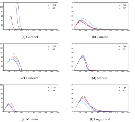
(ap-proximately yearly); which correspond to96, 48and12pricing periods respectively. We will refer to these three setups as Setup50, Setup100, and Setup400 respectively when we present our results. The three experimental setups reflect different price revision opportu-nities. The rationale for choosing the setups in this way also comes from the toll-pricing motivation. In Figure 1 and Figure 2, we show the shape of revenue and usage curves versus the price respectively for a sample of 5 instances out of 100 used from each dis-tribution type. We also depict the converged prices of both algorithms on these curves.
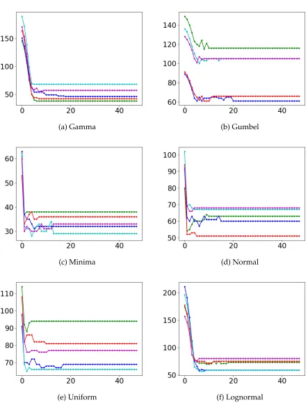
Figure 3gives the price paths of the same five instances.
4.3.2 DJA vs BZ
To evaluate BZ we have considered several combinations ofτ (learning time) andη (num-ber of prices to explore), shown in Table 3, and report the lowest average regret ob-tained over all these parameter combinations. We compare this (optimized) BZ to the (non-optimized) DJA with the following default parameters: U U = 0.25, τDJA = 20,
Distribution/Data Parameters Gumbel [20 : 50,2]
Gamma [3 : 5,13 : 15]
Uniform [30 : 80,120 : 170]
Normal [90 : 110,10 : 30]
Minima *
[image:25.612.72.295.78.191.2]Log-Normal [15 : 12,15 : 12]
Table 1: Parameter Ranges
Distribution/Data Parameters Gamma [3 : 5,13 : 15]
Uniform [50 : 99,100 : 150]
Normal [90 : 110,10 : 30]
Log-Normal [15 : 12,15 : 12]
[image:25.612.310.533.83.193.2]Beta [2 : 5,2 : 5]
Table 2: Data for minima distribution
50 100 150 200 250 300 350 400 450 0 20 40 60 80 100 120 DJA BZ (a) Gumbel
50 100 150 200 250 300 350 400 450 0 20 40 60 80 100 120 DJA BZ (b) Gamma
50 100 150 200 250 300 350 400 450 0 20 40 60 80 100 120 DJA BZ (c) Uniform
50 100 150 200 250 300 350 400 450 0 20 40 60 80 100 120 DJA BZ (d) Normal
50 100 150 200 250 300 350 400 450 0 20 40 60 80 100 120 DJA BZ (e) Minima
50 100 150 200 250 300 350 400 450 0 20 40 60 80 100 120 DJA BZ (f) Lognormal
[image:25.612.90.539.243.647.2]50 100 150 200 250 300 350 400 450 0.0 0.2 0.4 0.6 0.8 1.0 DJA BZ (a) Gumbel
50 100 150 200 250 300 350 400 450 0.0 0.2 0.4 0.6 0.8 1.0 DJA BZ (b) Gamma
50 100 150 200 250 300 350 400 450 0.0 0.2 0.4 0.6 0.8 1.0 DJA BZ (c) Uniform
50 100 150 200 250 300 350 400 450 0.0 0.2 0.4 0.6 0.8 1.0 DJA BZ (d) Normal
50 100 150 200 250 300 350 400 450 0.0 0.2 0.4 0.6 0.8 1.0 DJA BZ (e) Minima
[image:26.612.92.537.105.507.2]50 100 150 200 250 300 350 400 450 0.0 0.2 0.4 0.6 0.8 1.0 DJA BZ (f) Lognormal
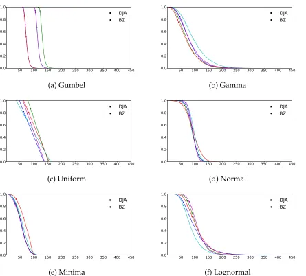
Figure 2: Usage vs Price plots for 5 instances of data generated from different distributions
τ 10 12 14 15 16 18 20
η 2, 5, 10 2, 3, 4, 6, 12 2, 7, 14 3, 5, 15 2, 4, 8, 16 2, 3, 6, 9, 18 2, 4, 5, 10, 20
[image:26.612.97.516.602.636.2](a) Gamma (b) Gumbel
(c) Minima (d) Normal
[image:27.612.78.521.81.664.2](e) Uniform (f) Lognormal
Gamma Gumbel Minima Normal Uniform Lognormal
DJA 37.76 (4.10) 18.50 (1.55) 26.99 (20.71) 26.33 (20.31) 12.46 (3.27) 27.73 (2.70) BZ 34.75 (6.21) 63.58 (9.03) 21.65 (4.19) 24.19 (3.85) 15.36 (3.17) 45.23 (13.51)
(a) Setup400
Gamma Gumbel Minima Normal Uniform Lognormal
DJA 13.49 (2.45) 12.28 (1.76) 13.13 (3.56) 12.00 (3.42) 8.55 (3.61) 11.76 (1.83) BZ 18.43 (3.02) 28.28 (10.49) 12.74 (2.74) 12.82 (3.02) 9.83 (3.28) 17.88 (2.73)
(b) Setup100
Gamma Gumbel Minima Normal Uniform Lognormal
DJA 12.40 (2.99) 10.54 (2.31) 13.27 (3.84) 10.39 (3.63) 7.52 (3.17) 9.72 (1.98) BZ 11.31 (3.56) 21.36 (11.28) 8.90 (3.64) 8.35 (2.44) 7.86 (4.08) 11.13 (2.36)
[image:28.612.85.526.71.284.2](c) Setup50
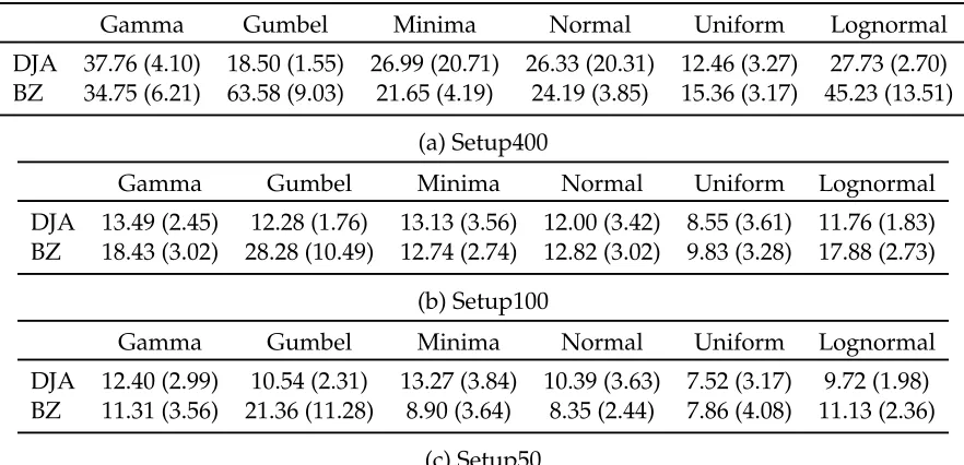
Table 4: Comparison DJA vs BZ
the standard deviations for both algorithms. As expected, the average regrets are highest in Setup400 due to very small opportunity to learn. Also, the variability is higher in this setup compared to the other two.
In all the cases the performance of (non-optimized) DJA is competitive to (optimized) BZ. In cases of Gumbel and Uniform DJA always outperforms BZ, while in other cases DJA without even parameter optimization comes close to BZ. The high standard devia-tions of DJA in Setup400 are due to the fact that the problem does not offer sufficient time to find the near optimal price.
As will be seen in subsequent sections, a bit of parameter tuning and judicious setting improves DJA’s performance considerably.We will defer the discussion on performance improvement to later sections and first consider incoporating the price caps into the pric-ing algorithms.
4.3.3 Price Caps
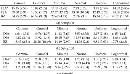
Gamma Gumbel Minima Normal Uniform Lognormal
DJA* 15.45 (9.54) 15.82 (2.05) 11.11 (2.98) 7.23 (3.28) 3.41 (2.58) 14.53 (5.85) DJA 39.30 (3.95) 18.50 (1.57) 27.37 (12.22) 23.50 (10.64) 12.49 (3.26) 28.08 (2.85) BZ 34.75 (6.21) 63.58 (9.03) 22.67 (4.19) 23.39 (3.3) 15.24 (3.18) 45.23 (13.51)
(a) Setup400
Gamma Gumbel Minima Normal Uniform Lognormal
DJA* 6.04 (1.34) 10.76 (4.07) 11.43 (3.69) 5.59 (3.38) 3.17 (2.18) 6.45 (1.61) DJA 14.82 (3.04) 11.92 (1.48) 15.25 (3.86) 12.55 (3.66) 8.41 (3.58) 11.86 (1.93) BZ 18.43 (2.51) 28.28 (10.49) 14.49 (2.90) 14.98 (2.2) 9.81 (3.03) 17.78 (2.43)
(b) Setup100
Gamma Gumbel Minima Normal Uniform Lognormal
DJA* 5.16 (1.40) 9.68 (3.96) 11.15 (4.01) 4.75 (3.55) 3.55 (2.21) 5.18 (1.54) DJA 13.80 (3.40) 9.86 (2.19) 15.14 (4.45) 11.91 (4.43) 7.23 (3.21) 9.97 (2.11) BZ 11.28 (3.29) 21.36 (11.28) 9.46 (3.27) 9.53 (1.54) 7.79 (3.9) 11.12 (2.31)
[image:29.612.86.525.72.323.2](c) Setup50
Table 5: Comparison DJA vs BZ with price cap of5%
We compare the performance of both algorithms on same data in the presence of cap constraint. The cap value is set at5%. Table 5gives the summary of results of outputs of algorithms in the presence of cap. Note that the table includes also performance of DJA*, which will be discussed insubsection 5.5.
In comparison with the no-cap case, the performance of both algorithms is, approxi-mately, similar when starting at high price, with a decrease in average regret for some dis-tributions and the opposite in others. Note that here again we compare the non-optimized DJA with optimized BZ. As we mentioned in the last section, starting at good price can achieve much better performance for DJA which is even more important in the presence of price caps. To illustrate, we show the average regret growth curves for three different strating prices (Q4 > Q3 > Q2— explained in Section 5) in DJA versus BZ in Figure 4
(a) Gamma (b) Gumbel
(c) Minima (d) Normal
[image:30.612.80.520.85.651.2](e) Uniform (f) Lognormal
4.4
Real data
In real world the travel times and hence costs may not have any known distribution which can be analytically expressed and may have seasonality and trends over time. Moreover, a model which performs well on simulated data may not perform well on real data. To test our approach on real data which as we explain below is given as travel times on a real road network, we assume the cost is proportional to the travel times. We first explain the details of data collection and then give then details of experimental setup and results.
4.4.1 Data Collection and Cleaning
We used data provided by the City of Chicago(https://data.cityofchicago.org), which provides a live traffic data interface. We recorded traffic updates in a 15-minute interval over a time horizon of 24 hours for several days between March 28th 2017 to May 12th 2017. A total of 4,363 data observations were used.
Every observation contains the traffic speed for a subset of a total of 1,257 segments. There were 1,045 segments where the data was recorded at least once of the 4,363 time points with almost all segments having at least 400 records. We used linear interpolation to fill the missing records keeping in mind that data was collected over time. Segment lengths were given through longitude and latitude coordinates, and approximated using the Euclidean distance.
As segments are purely geographical objects without structure, some processing has been done to create a graph. For the sake of space we omit including the graph plot here, instead we refer the interested reader to [8]. The final graph contains 538 nodes and 1,308 arcs.
4.4.2 Experimental Setup, Results and Discussion
We assume cost of travel on each road in this network is proportional to the time of travel. Since there are no toll roads in this network which we can use for our experiments we have randomly selected 100 pairs of cities and calculated tolls by imagining a toll road between each of these pair of cities, under the assumption that cost other than tolls is zero or such costs have been adjusted in the costs of the other roads. Of 4,463 observations we used 4,400 data points with price revision points for every 100 time points.
com-Relative regret Cap on Cap off Average 8.09 8.25 Stdev 4.23 3.99
Table 6: Results for Chicago data withU U = 0.30andp(0) =Q2
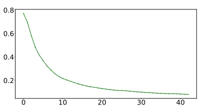
0 10 20 30 40
0.2 0.4 0.6 0.8
Figure 5: Chicago dataset: relative regret growth.
pared to that of when there is no constraint. Figure 5gives the change in average relative regret with respect to time.
5
Sensitivity Analysis
In this Section we study the impact of changing the algorithm parameters on the per-formance of the DJA Algorithm. More specifically by choosing the price and confidence level at right levels the performance of DJA improves to a large extent and outperforms BZ in almost all cases.
5.1
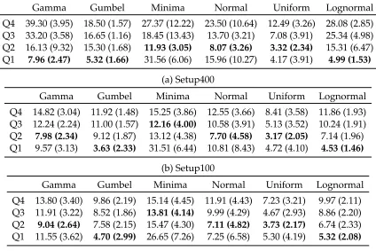
Impact of Starting price
[image:32.612.203.424.168.278.2][ω2, ωJ−1]. As can be noted from the Table 7, starting prices have considerable impact
on the performance of the algorithm. Especially, in the case of Minima distribution this impact is more compared to other cases. While in all three setups and for all distributions Q1 price seem to give lowest average regrets, except in case of Minima, this may be a risky strategy especially when there is a price cap.
When there are more periods, in Setup50 (Table 7(c)), except for Minima, for all distri-butions algorithm gives a very good performance when starting price is chosen at Q2 and Q3. Table 7(b) shows that starting at a good price can offset the difficulty of less peiods. Particularly interesting are the results in Setup400, where there are less chances of price revision and hence less opportunity for optimal learning, it is noteworthy that at Q2 the regrets are much more competitive than when starting high. In all the distributions on av-erage the optimal price seem to lie between Q2 and Q1 prices, again the exception being Minima.
For the experiments of Table 7 we fixed all the parameters same as in subsubsec-tion 4.3.3i.e., we set(1−α)at0.95,τDJAat20%T, UU at 0.25.
Since Algorithm DJA uses all the history, unlike algorithms which only use data from experimentation phase, the price path is dynamically selected. As can be seen inTable 7
the performance of DJA Algorithm is much better when the initial price is set at the me-dian price.
(a) Minima: Setup50 (b) Minima: Setup100
Figure 6: Price paths comparison for Minima: Setup50 vs Setup400
Gamma Gumbel Minima Normal Uniform Lognormal
Q4 39.30 (3.95) 18.50 (1.57) 27.37 (12.22) 23.50 (10.64) 12.49 (3.26) 28.08 (2.85) Q3 33.20 (3.58) 16.65 (1.16) 18.45 (13.43) 13.70 (3.21) 7.08 (3.91) 25.34 (4.98) Q2 16.13 (9.32) 15.30 (1.68) 11.93 (3.05) 8.07 (3.26) 3.32 (2.34) 15.31 (6.47) Q1 7.96 (2.47) 5.32 (1.66) 31.56 (6.06) 15.96 (10.27) 4.17 (3.91) 4.99 (1.53)
(a) Setup400
Gamma Gumbel Minima Normal Uniform Lognormal
Q4 14.82 (3.04) 11.92 (1.48) 15.25 (3.86) 12.55 (3.66) 8.41 (3.58) 11.86 (1.93) Q3 12.24 (2.24) 11.00 (1.57) 12.16 (4.00) 10.58 (3.91) 5.13 (3.52) 10.24 (1.91) Q2 7.98 (2.34) 9.12 (1.87) 13.12 (4.38) 7.70 (4.58) 3.17 (2.05) 7.14 (1.96) Q1 9.57 (3.13) 3.63 (2.33) 31.51 (6.44) 10.81 (8.43) 4.72 (4.10) 4.53 (1.46)
(b) Setup100
Gamma Gumbel Minima Normal Uniform Lognormal
Q4 13.80 (3.40) 9.86 (2.19) 15.14 (4.45) 11.91 (4.43) 7.23 (3.21) 9.97 (2.11) Q3 11.91 (3.22) 8.52 (1.86) 13.81 (4.14) 9.99 (4.29) 4.67 (2.93) 8.86 (2.20) Q2 9.04 (2.64) 7.58 (2.15) 15.47 (4.30) 7.11 (4.82) 3.73 (2.17) 6.74 (2.33) Q1 11.55 (3.62) 4.70 (2.99) 26.65 (7.26) 7.25 (6.58) 5.30 (4.19) 5.32 (2.08)
(c) Setup50
[image:34.612.94.518.352.635.2]5.2
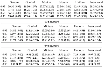
Impact of confidence level
The confidence bound calculated in the estimation phase is a control parameter in our algorithm which controls and captures the risk attitude of the toll-setter/decision maker. A risk averse toll-setter may set the α at a low level to increase the confidence level. This implies the price decisions should be more conservative. On the other hand less risk averse seller may choose to set a more modest level of α. This is also observed in the average regrets give in Table 8, where we report the performances against different levels of confidence from0.5%to0.95%. We observe that the regrets are the least (almost in all cases) at the lower level of confidence. The effect is more pronounced for some distributions than others. Two exceptions being Gumbel and Uniform. In Gumbel case, the prices (and the optimal) are in the lower tails of price range. We noticed that the price paths with varying level of confidence are not significantly different and it is most likely that the difference in performance is likely by chance of randomness. Similarly in the Uniform case the difference in the performance is very insignificant. As one would expect the effect of lower confidence would be more visible in the case with more periods. The variance in regrets increases with decreasing confidence, this is representative of the risk or loss of confidence as one may expect.
5.3
Impact of
τ
DJAParameterτDJAis used to control the maximum duration of the Forced Exploration phase of DJA algorithm. The Forced Exploration phase ends either because of observing a usage greater than UU or because of reaching (or exceeding) its maximum duration, in which casep(i)is set toω
2.
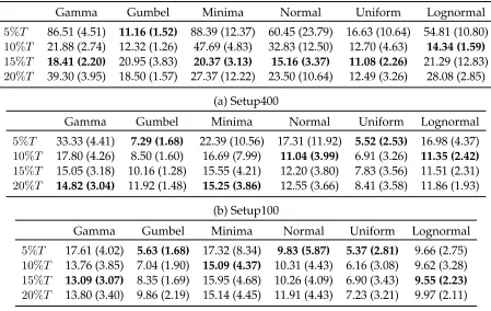
In Section 4, τDJA was set to20%T. Table 9 illustrates the sensitivity of the algorithm
to this parameter, by comparing it to three shorter maximum durations,5%T, 10%T and
15%T. Table 9(c) indicates that in Setup50, where there are many short pricing periods, the algorithm is generally quite robust, although it is important to note that10%T and15%T
almost always outperform20%T. The preference between5%T and10%T is inconclusive, as it is distribution-dependent.
As the number of pricing periods decreases, see Table 9(b), performance gains from decreasing τDJA to10%T or15%T become inconclusive, and decreasing to 5%T leads to
Gamma Gumbel Minima Normal Uniform Lognormal 0.95 39.30 (3.95) 18.50 (1.57) 27.37 (12.22) 23.50 (10.64) 12.49 (3.26) 28.08 (2.85) 0.80 37.40 (4.59) 18.26 (1.36) 26.76 (12.38) 23.08 (10.58) 12.55 (3.35) 27.47 (2.90) 0.65 36.15 (4.35) 18.15 (1.35) 26.77 (12.35) 22.65 (10.47) 12.49 (3.21) 26.92 (2.84) 0.50 35.05 (4.45) 17.88 (1.15) 26.32 (12.64) 22.27 (10.65) 12.62 (3.51) 26.65 (2.97)
(a) Setup400
Gamma Gumbel Minima Normal Uniform Lognormal
0.95 14.82 (3.04) 11.92 (1.48) 15.25 (3.86) 12.55 (3.66) 8.41 (3.58) 11.86 (1.93) 0.80 12.97 (2.51) 12.26 (2.21) 13.78 (3.53) 11.58 (3.12) 8.66 (4.04) 10.85 (1.67) 0.65 12.16 (2.40) 12.58 (2.28) 13.17 (3.75) 10.81 (2.82) 8.91 (4.06) 10.49 (1.32) 0.50 11.70 (2.46) 12.96 (2.74) 12.41 (2.92) 10.69 (2.99) 8.92 (4.17) 10.39 (1.35)
(b) Setup100
Gamma Gumbel Minima Normal Uniform Lognormal
0.95 13.80 (3.40) 9.86 (2.19) 15.14 (4.45) 11.91 (4.43) 7.23 (3.21) 9.97 (2.11) 0.80 11.19 (2.54) 9.93 (2.27) 12.74 (3.75) 10.49 (3.71) 7.76 (3.72) 8.76 (1.53) 0.65 10.05 (1.96) 10.40 (2.60) 11.84 (3.52) 9.50 (2.98) 7.93 (3.74) 8.34 (1.30) 0.50 9.10 (1.72) 10.39 (2.78) 10.47 (3.15) 9.38 (3.09) 8.24 (4.02) 8.11 (1.28)
[image:36.612.92.523.214.497.2](c) Setup50
Gamma Gumbel Minima Normal Uniform Lognormal
5%T 86.51 (4.51) 11.16 (1.52) 88.39 (12.37) 60.45 (23.79) 16.63 (10.64) 54.81 (10.80) 10%T 21.88 (2.74) 12.32 (1.26) 47.69 (4.83) 32.83 (12.50) 12.70 (4.63) 14.34 (1.59)
15%T 18.41 (2.20) 20.95 (3.83) 20.37 (3.13) 15.16 (3.37) 11.08 (2.26) 21.29 (12.83) 20%T 39.30 (3.95) 18.50 (1.57) 27.37 (12.22) 23.50 (10.64) 12.49 (3.26) 28.08 (2.85)
(a) Setup400
Gamma Gumbel Minima Normal Uniform Lognormal
5%T 33.33 (4.41) 7.29 (1.68) 22.39 (10.56) 17.31 (11.92) 5.52 (2.53) 16.98 (4.37) 10%T 17.80 (4.26) 8.50 (1.60) 16.69 (7.99) 11.04 (3.99) 6.91 (3.26) 11.35 (2.42)
15%T 15.05 (3.18) 10.16 (1.28) 15.55 (4.21) 12.20 (3.80) 7.83 (3.56) 11.51 (2.31) 20%T 14.82 (3.04) 11.92 (1.48) 15.25 (3.86) 12.55 (3.66) 8.41 (3.58) 11.86 (1.93)
(b) Setup100
Gamma Gumbel Minima Normal Uniform Lognormal
5%T 17.61 (4.02) 5.63 (1.68) 17.32 (8.34) 9.83 (5.87) 5.37 (2.81) 9.66 (2.75) 10%T 13.76 (3.85) 7.04 (1.90) 15.09 (4.37) 10.31 (4.43) 6.16 (3.08) 9.62 (3.28) 15%T 13.09 (3.07) 8.35 (1.69) 15.95 (4.68) 10.26 (4.09) 6.90 (3.43) 9.55 (2.23)
[image:37.612.81.530.71.355.2]20%T 13.80 (3.40) 9.86 (2.19) 15.14 (4.45) 11.91 (4.43) 7.23 (3.21) 9.97 (2.11) (c) Setup50
Table 9: Performance of DJA Algorithm at different values ofτ(DJA)
set are p(0) = ω
J−1, p(1) ≈ (ωJ−1 +ω2)/2, and p(2) = ω2. The negative effect of
decreas-ing τDJA is even more pronounced if there are even fewer pricing periods, as shown in Table 9(a). Note that in case 5%T, the algorithm spends at most2pricing periods in the Forced Exploration phase, in which case the prices set arep(0) = ω
J−1,p(1) = ω2.
Overall, only Gumbel distribution benefits from very small value of τDJA, which is because the optimal price is very close to the lowest allowable priceqand because all the prices in the neighbourhood ofqand of the optimal price yield nearly-optimal revenue.
5.4
Impact of UU
setter believes is enough usage to get good revenues. The impact of the level of UU is dif-ferent in all distributions, with no particular pattern true for all distributions and seems also to vary between setups.
Table 10suggests that for a fixedτDJAin case of larger period duration lower UU
suf-fices whereas for shorter durations higher values of UU are required to allow for sufficient exploration. This can be ascertained to the fact that rate of price decrease in forced explo-ration phase is roughly proportional to period duexplo-ration. For example, in Setup50 the best results are obtained at 0.35. In almost all cases, UU set at 0.05 does not give enough room for better exploration of the price range, resulting in overly conservative prices with higher variability in performance.
To cover for the sensitivity of the algorithm to UU, it is conceivable that a dynamic UU rule may be incorporated which also updates UU with each observation. Irrespectively of the setup, Minima and Normal distributions seem to be more sensitive to changes in UU levels compared to the other distributions. One explanation for these other distributions, except for Uniform, seems that they are more skewed and that the price ranges for these distributions are also different.
5.5
Discussion
The dynamic and adaptive nature of DJA allows it to avoid unattractive prices if good starting price is chosen, and this feature of the algorithm is extremely important in the presence of price caps. Similarly, the level of conservatism captured by confidence level takes into account the decision maker’s risk appetite and is useful in avoiding overly conservative prices even without the knowledge of the distribution. The analysis in sub-section 5.1–subsection 5.4illustrates the gain in the performance that can be achieved by tuning the input parameters to better values. Of course, which parameter values are bet-ter depends on the distribution family, the knowledge of which even without knowing the exact distribution parameters can help in making the right choice for values of input pa-rameters. Table 7–Table 10indicate that it is preferable to choose starting values between Q2 and Q3; αlevel at 0.5;τDJAbetween15%T and 20%T; and UU between0.25and 0.35
in order to improve the performance across all distributions, even though in some cases there may be other choices that give better performance for a particular distribution.
UU Gamma Gumbel Minima Normal Uniform Lognormal
0.05 39.01 (4.87) 18.54 (1.56) 19.98 (6.78) 19.34 (3.84) 12.49 (3.26) 27.61 (3.58)
0.15 39.30 (3.95) 18.50 (1.57) 21.15 (7.18) 19.74 (5.63) 12.49 (3.26) 28.08 (2.85) 0.25 39.30 (3.95) 18.50 (1.57) 27.37 (12.22) 23.50 (10.64) 12.49 (3.26) 28.08 (2.85) 0.35 39.30 (3.95) 18.50 (1.57) 35.02 (12.52) 31.97 (13.86) 12.49 (3.26) 28.08 (2.85)
(a) Setup400
UU Gamma Gumbel Minima Normal Uniform Lognormal
0.05 15.52 (3.14) 11.69 (1.48) 19.83 (6.40) 14.24 (4.45) 7.83 (3.17) 12.06 (1.77) 0.15 14.99 (3.24) 11.69 (1.26) 16.50 (4.80) 12.59 (3.86) 8.29 (3.52) 11.81 (1.85)
0.25 14.82 (3.04) 11.92 (1.48) 15.25 (3.86) 12.55 (3.66) 8.41 (3.58) 11.86 (1.93) 0.35 14.79 (3.04) 11.91 (1.51) 15.00 (3.96) 12.42 (3.54) 8.73 (4.12) 11.97 (1.94)
(b) Setup100
UU Gamma Gumbel Minima Normal Uniform Lognormal
0.05 26.65 (19.39) 9.40 (1.89) 28.62 (16.24) 15.57 (13.80) 7.39 (7.27) 13.81 (9.11) 0.15 14.47 (3.93) 9.45 (2.09) 17.62 (5.07) 12.55 (4.52) 6.88 (2.79) 10.41 (2.13) 0.25 13.80 (3.40) 9.86 (2.19) 15.14 (4.45) 11.91 (4.43) 7.23 (3.21) 9.97 (2.11) 0.35 13.34 (3.14) 9.81 (2.29) 14.29 (3.84) 10.35 (3.75) 7.49 (3.48) 9.82 (2.03)
[image:39.612.89.524.220.500.2](c) Setup50
following parameter values: starting price at Q2, α at 0.5, τDJA at20%T and UU at0.25.
Note that a full enumeration of all combinations of potential values of the parameters could lead to an even better performing, optimized, version of our algorithm.
6
Conclusion
We have presented a novel algorithm for dynamic pricing when the demand function is unknown. The algorithm balances the trade-off between price experimentation and revenue maximization, and has been derived by incorporating a novel conservative esti-mation of the alternative product cost distribution together with a novel non-adversarial robust optimization approach for pricing. The algorithm is flexible to incorporate addi-tional constraints, such as price caps, and performs competitively to an optimized version of a state-of-the-art algorithm that is asymptotically optimal.
Although we have presented the model for a variant, in which there is a single cus-tomer that makes repetitive purchasing decisions during every pricing period, the results also apply to another variant, in which there is a known number of customers purchasing in every period. We also believe that an adaptation of the proposed algorithm would per-form competitively if the number of customers purchasing in every period is unknown. Minor modifications would be needed to remove the dependence of all the quantities on
N(i).
In the estimation step, DJA employs the widely popular normal approximation in the construction of the confidence intervals. This works very well when the period durations are large, but, as the results in the previous section illustrate, the confidence intervals con-structed are very sensitive to the period duration. To deal with this sensitivity, one option to look at are other ways of constructing the confidence interval, like Jeffrey’s interval, Clopper-Pearson interval, etc. This is especially important when one is constrained to update price at short intervals.