Object recognition and real time tracking in microscope imaging

Object recognition and real-time tracking in microscope

imaging

WEDEKIND, Jan, BOISSENIN, Manuel, AMAVASAI, Balasundram P.,

CAPARRELLI, Fabio and TRAVIS, Jon R.

Available from Sheffield Hallam University Research Archive (SHURA) at:

http://shura.shu.ac.uk/3738/

This document is the author deposited version. You are advised to consult the

publisher's version if you wish to cite from it.

Published version

WEDEKIND, Jan, BOISSENIN, Manuel, AMAVASAI, Balasundram P., CAPARRELLI,

Fabio and TRAVIS, Jon R. (2006). Object recognition and real-time tracking in

microscope imaging. In: Proceedings of the 2006 Irish Machine Vision and Image

Processing Conference (IMVIP 2006). Dublin, Vision System Group, 164-171.

Copyright and re-use policy

See

http://shura.shu.ac.uk/information.html

Object Recognition and Real-Time Tracking in

Microscope Imaging

J. Wedekind, M. Boissenin, B.P. Amavasai, F. Caparrelli, J. Travis

MMVL, Materials and Engineering Research Institute

Sheffield Hallam University,

Pond Street,

Sheffield S1 1WB

{

J.Wedekind,B.P.Amavasai,F.Caparrelli,J.R.Travis

}

@shu.ac.uk,

[email protected]

30.6.2006

Abstract

As the fields of micro- and nano-technology mature, there is going to be an increased need for industrial tools thatenable the assembly and manipulation of micro-parts. The feedback mechanism in a future micro-factory will require computer vision.

Within theEU IST MiCRoNproject, a computer vision software based onGeometric Hashing

and theBounded Hough Transformto achieverecognition of multiple micro-objectswas imple-mented and successfully demonstrated. In this environment, the micro-objects will be of variable distance to the camera. Novel automated procedures in biology and micro-technology are thus con-ceivable.

This paper presents an approach to estimate the pose of multiple micro-objects with up to four degrees-of-freedom by using focus stacks as models. The paper also presents a formal definition for Geometric Hashing and the Bounded Hough Transform.

Keywords:object recognition, tracking, Geometric Hashing, Bounded Hough Transform, microscope

1

Introduction

Under the auspices of the EuropeanMiCRoN[MiCRoN consortium, 2006] project a system of multiple micro-robots for transporting and assemblingµm-sized objects was developed. The micro-robots are about 1cm3_{in size and are fitted with an interchangeable toolset that allows them to perform} manipula-tion and assembly. The project has developed various subsystems for powering, locomomanipula-tion, posimanipula-tioning, gripping, injecting, and actuating. The task of theMicrosystems & Machine Vision Labwas to develop a real-time vision system, which provides feedback information to the control system and hence forms part of the control loop.

Although there are various methods for object recognition in the area of computer vision, most techniques which have been developed for microscope imaging so far do not address the issue of real-time. Most current work in the area of micro-object recognition employs 2-D recognition methods (see

e.g. [Begelman et al., 2004]) sometimes in combination with an auto-focussing system, which ensures that the object to be recognised always stays in focus.

This paper presents an algorithm for object recognition and tracking in a microscope environment with the following objectives: Objects can be recognised withup to 4 degrees-of-freedom,refocussing is not required,tracking is performed in real-time.

The following sections of this paper will provide a formalism toGeometric Hashingand theBounded Hough Transform, how they can be applied to a pre-stored focus stack, and how this focus stack can be used to recognise and track objects, the results, and finally we draw some conclusions.

2

Formalism

2.1

Geometric Hashing

[Forsyth and Ponce, 2003] provides a complete description of the Geometric Hashing algorithm first introduced in [Lamdan and Wolfson, 1988]. Geometric Hashing is an algorithm that uses geometric invariants to vote for feature correspondences.

2.1.1 Preprocessing-Stage

Let the triplet~p:= (t1, t2, θ)⊤ ∈P be the pose of an object andP :=R3the pose-space.dim(P) = 3 is the number of degrees-of-freedom. The object can rotate around one axis and translate in two directions. It can be found using a setM ⊂Rd+1_{of homogeneous coordinates denoting 2-D (d= 2)} feature points (here: edge-points acquired with a Sobel edge-detector) as a model

M :=m~i= (mi,1, mi,2,1)⊤i∈ {1,2, . . .} (1) First the set of geometric invariantsL(M)has to be identified. A geometric invariant of the model is a feature or a (minimal) sequence of features such that the pose of the object can be deduced if the location of the corresponding feature/the sequence of features in the scene is known.

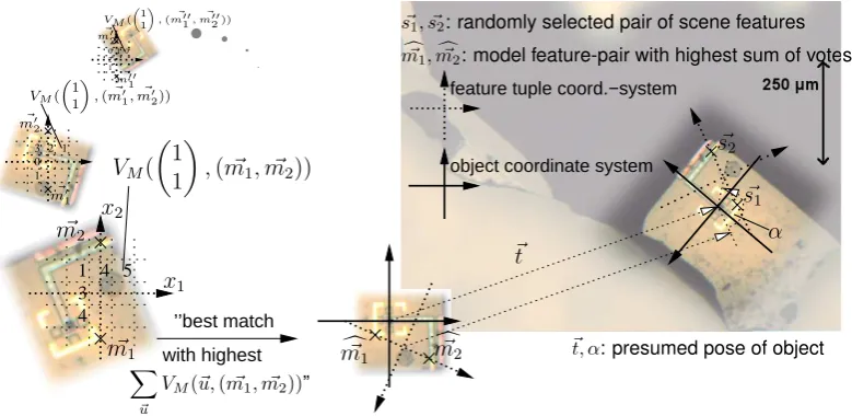
Consider the example in fig. 1. In this case the correspondence between a two feature pointss~1, ~s2∈

Sin the sceneS⊂Rd+1_{and two feature pointsm~}

1, ~m2∈M of the modelM would reveal the pose~p of the object. Therefore feature tuples can serve as geometric invariants.

In practice only a small number of feature tuples can be considered. A subset ofM×Mis selected by applying a minimum- and a maximum-constraint on the distance between the two feature points of a tuple(l~1, ~l2). Hence in this case,Lis defined asL(A) =

(l~1, ~l2)∈A×A

gu≤ ||l~1−~l2|| ≤go for

any set of featuresA⊆Rd+1_.

X

~ u

VM(~u,(m~1, ~m2))”

V

(

1

1

,

(

m

~

, ~

m

))

VM(

„ 1 1 «

,(m~′ 1, ~m′2))

VM(

„

1 1

« ,(m~′′

1,m~′′2 ))

x

x

~

m

~

m

4

0 3 2 1 1

2 0 1 0 1

’’best match

with highest

c~

m1,mc~2: model feature-pair with highest sum of votes

~

s1, ~s2: randomly selected pair of scene features

~t, α: presumed pose of object

α ~t ~ s1 ~ s2 c~

m1 mc~2

feature tuple coord.−system

object coordinate system

Figure 1: Geometric Hashing to locate a syringe-chip (courtesy of IBMT, St. Ingbert) in a microscope image (reflected light) allowing three degrees-of-freedom

Geometric Hashing provides a technique to establish the correspondence between the geometric invariants(m~1, ~m2)∈L(M)and(s~1, ~s2)∈L(S)whereS, M ⊂Rd+1.

To apply Geometric Hashing a function

t:

_L(Rd+1_{) → R}(d+1)×(d+1) (l~n) 7→ T (l~n)

(2)

is chosen which assigns an affine transformation matrix T (l~n)

to a geometric invariant (l~n) := (l~1, ~l2, . . . ~ln)inL(M)⊂L(Rd+1)orL(S)⊂L(Rd+1). The affine transformation inverses the

trans-formation which is designated by the sequence of features(l~1, ~l2, . . . ~ln).E.g.in this casetmust fulfil

∀~p∈P,(~l1, ~l2)∈R3×R3: t (R(p~)·l~1,R(~p)·l~2)=R(~p)·t

(l~1, ~l2)

whereR(

 tt12

θ

 ) :=



cos(sin(θθ)) −cos(sin(θθ)) tt12

0 0 1

Furthermoret must conserve the pose-information,i.e. dim aff(t(L(Rd+1_{)) = dim(P)where} aff(X)is the affine hull ofX.

Note that~land~l′_{are homogeneous coordinates of points, and for simplification we can usel}

3 =

l′

3= 1. Using this, a possible choice fortis given by

t (~l, ~l′_)=p 1

(l′

1−l1)2+ (l

′

2−l2)2

 

l′

2−l2 l1−l1′ 0

l′

1−l1 l′2−l2 0

0 0 1

 

 

1 0 −1

2(l1+l

′

1)

0 1 −1

2(l2+l

′

2)

0 0 1

  (4)

The choosen transformationt (m~1, ~m2)maps the two feature points~land~l′ on thex2-axis as shown in figure 1.

Lethbe a quantising function for mapping real homogeneous coordinates of feature positions to whole-numbered indices of voting table bins of discrete size∆s:

h:

  

Rd+1 _→ Zd

~x 7→ ~uwhereui=

_x

i

xd+1∆s +1

2

, i∈ {1,2, . . . , d} (5)

[Blayvas et al., 2003] offers more information on how to choose the bin size∆sproperly. Note that

xd+1= 1sincehis going to be applied to homogeneous coordinates of points only.

First a voting tableVM :Zd×L(M)→N0for the modelM is computed (see alg. 1)1. In practice

VM only needs to be defined on a finite subset ofZd, whileL(M)is finite ifM is.

Algorithm 1: Creating a voting table offline, before doing recognition with the Geometric Hashing algorithm[Forsyth and Ponce, 2003]

Input: ModelM ⊂Rd+1

Output: Voting tableVM :Zd×L(M)→N0

/* Set all elements of VM to zero */

VM(·,·)7→0;

foreachgeometric invariant(m~n) = (m~1, ~m2, . . . , ~mn)∈L(M)do

foreachfeature pointm~′_{∈M do}

/* Compute index of voting table bin */

~u:=h(t (m~n)

·m~′_);

/* Add one vote for the sequence of features (m~n) */

VM ~u,(m~n)7→VM ~u,(m~n)+ 1;

end end

(t (m~1, ~m2)·m~′)is the position ofm~′ relatively to the geometric invariant(m~1, ~m2) ∈L(M). This relative position is quantised byhand assigned to~u.VM ~u,(m~1, ~m2)is the number of features residing in the bin of the voting table with the quantised position~urelative to the geometric invariant

~

m∈L(M).

2.1.2 Recognition-Stage

A random pair of features(s~1, ~s2)is picked from the Sobel-edges of the scene-image. All other features of the scene are mapped using the transformt (s~1, ~s2)(see alg. 2). The accumulatora is used to decide where both features are located on the object and whether they are residing on the same object at all.

On success, sufficient information to calculate the pose of the object is available. The pose~p = (t1, t2, θ)⊤of the object can be calculated using:

R(~p) =t (s~1, ~s2)

−1

t (mc~1,mc~2) (6)

2.2

Bounded Hough Transform

As Geometric Hashing alone is too slow to achieve real-time vision, a tracking algorithm based on the Bounded Hough Transform[Greenspan et al., 2004] was employed. Thus after a micro-object has been located, it can be tracked in consecutive frames with much lower computational cost.

Algorithm 2: The Geometric Hashing algorithm for doing object recognition[Forsyth and Ponce, 2003]

Input: Set of scene featuresS ⊂Rd+1

Output: Pose~pof object or failure Initialise accumulatora:L(M)→N_0;

Randomly select a geometric invariant(s~n) = (s~1, ~s2, . . . , ~sn)fromL(S);

foreachfeature pointss~′_∈Sdo

/* Compute index ~u of voting table bin */

~u:=h(t (s~n)

·s~′_);

foreach(m~n)∈L(M)do

/* Increase the accumulator using the voting table */

a (m~n)7→a (m~n)+VM(~u,(m~n));

end end

/* Find accumulator bin with maximum value */

(mc~n) := argmax (m~n)∈L(M)

a (m~n)

;

ifa (mc~n)is bigger than a certain thresholdthen /* t (s~n)

−1

t (mc~n) contains suggested pose of object. Back-project and verify before accepting the

hypothesis[Forsyth and Ponce, 2003] */

else

/* Retry by restarting algorithm or report failure */

end

2.2.1 Preprocessing-Stage

The basic idea of the Bounded Hough Transform is to transform the positions of all features~s∈Sto the coordinate-system defined by the object’s previous pose~p. If the speed of the object is restricted by

r1, r2, . . .(i.e. |p′i−pi| ≤ ri,~r ∈ Rdim(P)) and the change of pose is quantised byq1, q2, . . .(i.e.

∃k∈Z_:p′

i−pi=k qi,~q∈Rdim(P)), the problem of determining the new posep~′∈P of the object

is reduced to selecting an elementbd~:=p~′_{−~pfrom the finite setD⊂Pof pose-changes}

D:=d~∈P∀i∈ {1, . . . ,dim(P)}:|di| ≤ri ∧ ∃k∈Z:di=k qi (7)

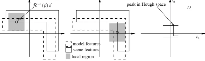
Fig. 2 illustrates how the Bounded Hough Transform works in the case of two degrees-of-freedom (p~= (t1, t2)⊤). The hough-space of pose-changesDis limited and therefore only the features residing within a small local area ofMcan correspond to the scene-feature~s∈S. Each possible correspondence

D R−1₍

~ p)~s

t1 t2

peak in Hough space

scene features model features

local region

Figure 2: Bounded Hough Transform with 2 degrees-of-freedom

votes for one pose-change (in the general case it may vote for several different pose-changes). As one can see in fig. 2, accumulating the votes of two scene-features already can reveal the pose-change of the object.

First a voting tableHM is computed as shown in alg. 3. In practiceHMonly needs to be defined on

a finite subset ofZd_{whileDis finite.}

Algorithm 3: Initialising voting table offline, before doing tracking using the Bounded Hough Transform algorithm

Input: ModelM ⊂Rd+1_{, ranges~r, quantisation~q}

Output: Voting tableHM :Zd×D→N0

/* Set all elements of HM to zero */

HM(·,·)7→0;

foreachpose difference vectord~∈Ddo foreachfeature pointm~ ∈M do

foreachpose difference vector~c∈C(m~)do

/* Compute index of voting table bin */

~u:=h(R(d~+~c)·m~);

/* Update votes for pose-change d~ */

HM(~u, ~d)7→HM(~u, ~d) +W(m~);

end end end

translation inDdoes not exceed the bin-size (i.e.qi≤∆s).

In the case of three degrees-of-freedom (~p = (t1, t2, θ)⊤) thedensityof the votes depends on the features distance from the origin (radius). If the radius is large, several bins ofHM may have to be

increased. If the radius is very small, the weight of the vote should be lower than1as the feature cannot define the amount of rotation unambiguously. Therefore in the general caseCandW are defined as follows

C(m~) :=~c∈P∀i∈ {1, . . . ,dim(P)}:|ci| ≤

qi 2

δR_δx(~x)

i

~

m ∧ ∃k∈Z_{:ci=k∆s (8)}

W(m~) = dim(P)

Y

i=1

min 1,δR(~x) δxi

~

m (9)

In the case of three degrees-of-freedomCandWare defined using

δR (t1, t2, θ)

⊤

δt1

~

m, δR (t1, t2, θ)

⊤

δt2

~

m,δR (t1, t2, θ)

⊤

δθ m~

⊤

=

 

m3

m3

p

m2 1+m22

 

(10) Note thatm~ is a homogeneous coordinate of a point and thereforem3= 1.

2.2.2 Tracking-Stage

The tracking-stage of the Bounded Hough Transform algorithm is fairly straightforward. All features of the scene are mapped using the transformR(~p)−1_{defined by the previous pose~pof the object (see alg.} 4). The accumulatorbis used to decide where the object has moved or whether it was lost.

2.3

Four Degrees-of-Freedom

In practice the depth information contained in microscopy images can be used to achieve object recogni-tion and tracking with four degrees-of-freedom. Recognirecogni-tion and tracking with four degrees-of-freedom is achieved by using two sets of competing voting tables{VM1, VM2, . . .}and{HM1, HM2, . . .}, which

have been generated from a focus stack of the object. Figure 3 shows an artificial focus stack of the text-object “Mimas”, which is being compared against an artificial image, which contains two text-text-objects.

The voting tables for recognition can be stored in a single voting tableV∗

M if an additional index

for the depth is introduced. Furthermore during tracking only a subset of{HM1, HM2, . . .}needs to be

considered as the depth of the object can only change by a limited amount. In practice an additional index for change of depth is introduced, and a set of voting tables{HM1,2, HM1,2,3, HM2,3,4, . . .} is

Algorithm 4: The Bounded Hough Transform algorithm for tracking objects

Input: Set of scene featuresS ⊂Rd+1_{, previous~pof object}

Output: Updated posep~′_{of object or failure}

Initialise accumulatorb:D→N_0; foreachfeature point~s∈Sdo

/* Compute index ~u of voting table bin _*/

~u:=h R(~p)−1_~s;

foreachvector of pose-changed~∈Ddo

/* Increase the accumulator using the voting table */

b(d~)7→b(d~) +HM(~u, ~d);

end end

/* Find accumulator bin with maximum value */

b~

d= argmax ~ d∈D

b(d~);

ifb(bd~)is bigger than a certain thresholdthen

/* p~′_=~p+b_d~ _{is the suggested pose of the object}

*/

else

/* Report failure */

end

Figure 3: Geometric Hashing with four degrees-of-freedom

Figure 4: Test environment

3

Results

In order to observe the tools and micro-objects, a custom built micro-camera was developed and mounted on a motorised stage (see fig. 4). The micro-camera has an integrated lens system and a built-in focus drive that allows the lens position to be adjusted. The field of view is similar to that obtained from a microscope with low magnification (about 0.8 mm×0.5 mm field of view).

The test environment (see fig. 4) allows the user to displace a micro-object using the manual trans-lation stage. The task of the vision-system is to keep the micro-object in the centre of the image and in focus using the motorised stage.

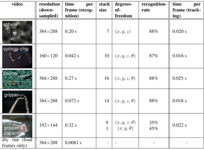
Figure 5 shows a list of results acquired on a 64-bit AMD processor with 2.2 GHz. The initialisation time for the voting-tables has not been included as they are computed offline. First recognition using geometric hashing was run on 1000 frames. Therecognition rateindicates the percentage of frames, when the object was recognised successfully. In a second test tracking was applied to 1000 frames. The last column in the table shows the corresponding improved frame-rate. In both tests the graphical visualisation was disabled (which saves 0.013 seconds per frame). To require less memory forVM and

HM, recognition and tracking are performed on down-sampled images. The disadvantage is that the

resulting pose-estimate for the micro objects is coarser.

tracking-Figure 5: Results for object recognition with Geometric Hashing in a variety of environments

video resolution (down-sampled)

time per frame (recog-nition)

stack size

degrees- of-freedom

recognition-rate

time per frame (track-ing)

384×288 0.20 s 7 (x, y, z) 88% 0.020 s

160×120 0.042 s 10 (x, y, z, θ) 87% 0.016 s

384×288 0.27 s 16 (x, y, z, θ) 88% 0.025 s

384×288 0.072 s 14 (x, y, z, θ) 88% 0.018 s

192×144 0.32 s 9

1

(x, y, z, θ) (x, y, θ)

35%

45% 0.022 s

dry run (load

frames only) 384×288 0.0081 s - - -

-rate (the complement of the recognition--rate) always is near 100%, a low recognition -rate does not necessarily affect the overall performance of the system.

The recognition rates are particularly low when the object is small, when the object has few features, when there is too much clutter in the scene image, or when multiple objects are present in the scene. The reason is that the final feature (or feature-tuple), which leads to a successful recognition of the object, needs to reside on the object. Furthermore both features of a feature-tuple need to reside on the same object. If all corresponding features to the features of the modelM are present in the sceneS, the probability of randomly selecting a suitable sequence of features is(|M|/|S|)n_.

The focus stack must not be self similar. For example the depth of the micro-capacitor in fig. 7 cannot be estimated independently because a planar object which is aligned with the focused plane will have the same appearance regardless whether it is moving upwards or downwards.

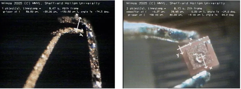
The grippers displayed in fig. 6 and 7 show a rough surface due to the etching step in the gripper’s manufacturing process. From a manufacturing point of view it would be desirable to smooth out this “unwanted” texture. This surface texture however led to the best of all results because it is rich with features.

As both recognition and tracking are purely combinatorial approaches, the memory requirements for the algorithms are high. In the case of the video showing the micro-gripper and the micro-capacitor, 130 MByte of memory was required for the tracking- and 90 MByte for the recognition-algorithm. State-of-the-art algorithms likeRANSAC (see [Fischler and Bolles, 1981]) use local feature context so that less features are required. RANSAC in combination with Linear Model Hashing also scales better with number of objects[Shan et al., 2004].

In Geometric Hashing, it is only feasible to compute VM from a small subset ofM ×M. By

considering only a part ofM, one can reduce the size ofHM in a similar fashion. ExperimentallyHM

was initialised only from features fulfilling||m~||q3≥1without affecting the tracking performance.

4

Conclusion

Figure 6: Micro camera image of gripper with uniform background with superimposed pose es-timate

Figure 7: Gripper placing a capacitor (courtesy of SSSA, Sant’ Anna) with superimposed pose esti-mates for gripper and capacitor

environment.

According to [Breguet and Bergander, 2001] the future micro-factory will most probably require automated assembly of micro-parts. The feedback mechanism for the robotic manipulators could be based on computer vision. A robust computer vision system which allows real-time recognition of micro-objects with 4 or more degrees-of-freedom would be desirable.

The algorithm presented in this paper has been implemented using the computer vision library of the

Microsystems & Machine Vision LabcalledMimas, which has been under development and refinement for many years. The library and the original software employed in the MiCRoN-project are available for free athttp://vision.eng.shu.ac.uk/mediawiki/under the terms of the LGPL.

References

[Begelman et al., 2004] Begelman, G., Lifshits, M., and Rivlin, E. (2004). Map-based microscope positioning. InBMVC 2004. Technion, Israel.

[Blayvas et al., 2003] Blayvas, I., Goldenberg, R., Lifshits, M., Rudzsky, M., and Rivlin, E. (2003). Geometric hashing: Rehashing for bayesian voting. Technical report, Computer Science Department, Technion Israel Institute of Technology.

[Breguet and Bergander, 2001] Breguet, J. M. and Bergander, A. (2001). Toward the personal factory? InMicrorobotics and Microassembly III, 29-30 Oct. 2001, Proc. SPIE - Int. Soc. Opt. Eng. (USA), pages 293–303.

[Fischler and Bolles, 1981] Fischler, M. A. and Bolles, R. C. (1981). Random sample consensus: a paradigm for model fitting with applications to image analysis and automated cartography. Commu-nications of the ACM, 24(6):381–95.

[Forsyth and Ponce, 2003] Forsyth, D. A. and Ponce, J. (2003).Computer Vision: A modern Approach. Prentice Hall series in artificial intelligence.

[Greenspan et al., 2004] Greenspan, M., Shang, L., and Jasiobedzki, P. (2004). Efficient tracking with the bounded hough transform. InCVPR’04: Computer Vision and Pattern Recognition.

[Lamdan and Wolfson, 1988] Lamdan, Y. and Wolfson, H. J. (1988). Geometric hashing: A general and efficient model-based recognition scheme. In Second International Conference on Computer Vision, Dec 5-8 1988, pages 238–249. Publ by IEEE, New York, NY, USA.

[MiCRoN consortium, 2006] MiCRoN consortium (2006). Micron public report. Technical report, EU IST-2001-33567.http://wwwipr.ira.uka.de/˜seyfried/MiCRoN/PublicReport_

Final.pdf.