GW4: a real-time background subtraction and maintenance
algorithm for FPGA implementation
APPIAH, Kofi <http://orcid.org/0000-0002-9480-0679>, HUNTER, Andrew and
KLUGE, Tino
Available from Sheffield Hallam University Research Archive (SHURA) at:
http://shura.shu.ac.uk/22198/
This document is the author deposited version. You are advised to consult the
publisher's version if you wish to cite from it.
Published version
APPIAH, Kofi, HUNTER, Andrew and KLUGE, Tino (2005). GW4: a real-time
background subtraction and maintenance algorithm for FPGA implementation.
WSEAS Transactions on Systems, 4 (10), 1741-1751.
Copyright and re-use policy
See
http://shura.shu.ac.uk/information.html
GW4: A Real-Time Background Subtraction and Maintenance Algorithm for
FPGA Implementation
KOFI APPIAH†
ANDREW HUNTER†
TINO KLUGE‡
Department of Computing and Informatics†
University of Lincoln
Lincoln, LN6 7TS
UK
OCIAM, Mathematical Institute‡
University of Oxford
Oxford, OX1 3LB
UK
{kappiah, ahunter}@lincoln.ac.uk, [email protected] http://facs.lincoln.ac.uk/Research/Vision
Abstract: - GW4 is a real-time video segmentation algorithm for detecting moving objects in indoor and outdoor scenes. The platform for the final implementation is Field Programmable Gate Array (FPGA); a reconfigurable computing platform. The algorithm detects moving foreground objects against a multimodal background; it is motivated by two well-known adaptive background differencing algorithms, Grimson's algorithm and W4. The implementation is based on a single stationary camera
transmitting RGB values at 25Hz. Background modelling at pixel level has been used in many applications, but normally fails due to camouflage and foreground aperture problems. These common problems have been reduced in our approach with the use of pixel and frame level processing. To make the algorithm feasible and efficient for the final hardware platform, we avoid the use of floating point numbers and transcendental operations. The final implementation operates at real-time frame rates on 640x480 video streams. We present experimental results indicating processing speeds, and superior segmentation performance to Grimson's algorithm for different values of K.
Key-Words: - FPGA, Multimodal background, Real-time processing, Reconfigurable hardware
1 Introduction
Video segmentation algorithms process large amount of data, and are consequently processor and memory hungry [11, 15]. Real-time robot vision tasks require high computational power and data throughput in order of magnitude, which far exceed those available on mainstream computer platforms [21]. Typically, image processing algorithms can be broke down into three major stages [3]: early processing, implemented by local pixel-level functions; intermediate processing, which includes segmentation, motion estimation and feature extraction; late processing, including interpretation and using statistical and artificial intelligence algorithms. Typically algorithmic sophistication is concentrated in the later stages, but processing demands are dominated by the early stages.
Background subtraction utilizes the visual properties of the scene for building an appropriate representation that can be use to identify foreground and background objects. Existing methods for background modelling can be classified as either predictive or non-predictive [22]. Predictive methods model the scene as a time series, while the non-predictive methods build a probability representation of the observation at pixel level. Limitations on processing power force us to use extremely simple algorithms for early processing, limiting performance. The proliferation of cheap sensor and increased processing power has made the
acquisition and processing of video information more feasible [20].
This article demonstrates how real-time early digital vision can be accomplished with the use of data and instruction parallelism. Our approach spans the early and intermediate levels described above. Most image segmentation algorithms are computationally expensive and require significant storage space; however, they are also often inherently parallelisable. Field Programmable Gate Array (FPGA) systems are ideal for the implementation of such algorithms, providing that algorithms are designed with the limitations of FPGA in mind (in particular, avoidance of floating point arithmetic is recommended). Modern FPGAs provide a very appealing platform for rapid, low-cost development of specialized algorithms, due to their reconfigurable nature, as opposed to older Application Specific Integrated Circuit (ASIC) designs, which have a very long and error-prone design cycle [1].
research interest in automated monitoring [5]. A number of algorithms for segmentation of moving objects have already been developed, and successfully implemented in software, at least for individual video streams at low frame rates and resolutions. Very few of these algorithms have been incorporated into today's video surveillance systems, partly due to computational complexity, cost and lack of real-time capability. “One might argue that there is always a bigger chip that will fit the application, but the use of reconfiguration may bring some other profits such as good system extensibility after the system expedition or more favourable power consumption”[23]. This makes the development of such algorithms on specialized hardware timely.
Multimodal background differencing segmentation algorithms are practical, reasonably fast and can handle some typical problems, such as camera jitter, moving foliage, water and lighting changes. They require a significant amount of floating point processing, and thus when implemented in software running on general-purpose computers are limited to low frame rates and small frame sizes. They typically absorb 80% to 90% of the entire processing time, which makes them unattractive for real-time purposes.
We present here a new multimodal background differencing segmentation algorithm, which is very simple, robust and can easily be implemented in computer hardware with maximum efficiency in terms of speed and hardware area. Our algorithm is a hybrid of two robust and well-known image segmentation algorithms (Grimson's, and W4), which
illustrates how simple algorithms can be designed for efficient FPGA implementation.
2 Previous Work
The first stage in processing for many video applications is the segmentation of (usually) moving objects. Where the camera is stationary, a natural approach is to model the background and detect foreground objects by differencing the current frame with the background. A wide and increasing variety of techniques for background modelling have been described; a good comparison is given by Gutchess et al [7]. The most popular method is unimodal background modelling, in which a single value is used to represent a pixel, which has been widely used due to its relatively low computational cost and memory requirements [8, 13]. This technique gives poor results when used in modelling non-stationary background scenarios like waving trees, rain and snow. A more powerful alternative is to use a multimodal background representation, the most common variant of which is a mixture of Gaussians [6, 12]. However, the computational demands make such techniques unpopular for real-time purposes; there are also disadvantages in multimodal techniques [6, 12, 13] including the blending effect, where a pixel attains an intensity value which has never occurred at that position (a side-effect of the smoothing
used in these techniques). Other techniques rely heavily on the assumption that the most frequent intensity value during the training period represents the background. This assumption may well be false, causing the output to have a large error level.
2.1 Grimson’s Algorithm
Grimson et al [12] introduced a multimodal approach, modelling the values of each pixel as a mixture of Gaussians. The background is modelled with the most persistent intensity values. The algorithm has two variants, colour and gray-scale: in this paper, we concentrate on the gray-scale version. The probability of observing the current pixel value is given as:
= = k i t i t i t t i t 1 , , , ( , , ) )(
(1)Where i,t, i,t and i,t are the respective mean, variance and
weight parameters of the ith Gaussian component of pixel at time t, and is a Gaussian probability density function
t i t i t e t i t i t i t , 2 , 2 ) ( , , , 2 1 ) , , ( − =
(2)A new pixel value is generally consistent with one of the major components of the mixture model and used to update the model. For every new pixel value, t, a check is
conducted to match it to one of the K Gaussian distributions. A match is found when t is within 2.5 standard deviations of
a distribution. If none of the K distributions match t, the
least weighed distribution is replaced with a new distribution having t as mean, high variance and very low weight. The
weights are updated as follows:
)
(
, , 11 ,
,t
=
it−+
it−
it−i
m
(3)where is the learning rate and
=
otherwise
0
match
a
is
there
if
1
,t im
(4)
1 defines the time constant which determines the speed at which the distribution's parameters change. Only the matched distribution will have its mean and variance updated, using the equations:
) (
1 t t t
t
)
(
*
)
(
)
1
(
t 1 t t T t tt
=
−
+
−
−
− (6)) , | (
t
t
t
= (7)The first B distributions (ordered by
k) are used as a model of the background, where) min( arg 1
= = b k k b TB
(8)The threshold T is a measure of the minimum portion of the data that should be accounted for by the background.
2.2 The W
4Algorithm
Haritaoglu et al [8] introduced the W4 algorithm, which uses
a single distribution with three integer values to model the background. Their background model requires manual initialisation; the three parameters (Maximum, Minimum and maximum inter-frame difference values) are acquired over a period of time (a few seconds) when there is no activity in the scene.
After the initialisation period, each pixel is classified as either a background or a foreground pixel using the background model. Given the maximum (M), minimum (m) and the largest inter-frame absolute difference (D) of the images collected over the initialisation period, a new pixel x from an image sequence It is a foreground pixel if:
) ( | ) ( ) (
|m x −It x D x (9)
or ) ( | ) ( ) (
|M x −It x D x (10)
In order to detect people in outdoor scenes using W4,
Haritaoglu et al [16] used new background modelling parameters and updating equations. The initial background model for a pixel at location x, is given as:
−
=
−|}
)
(
)
(
{|
max
)}
(
{
max
)}
(
{
min
)
(
)
(
)
(
1x
V
x
V
x
V
x
V
x
d
x
n
x
m
s s s s s s s (11)Where |Vs(x)−
(x)|2*
(x), for (x)and ) ( ),
(x
x
Vs being the respective stationary pixel value, standard deviation and median value of intensities at pixel location x. The assumption that the background model stays unchanged for long periods of time does not hold for outdoor scenes and hence must be updated periodically. A change map consisting of three components (detection support map gS, motion support map mS and change history
map hS) is dynamically constructed to determine whether a pixel-based or an object based update method applies. The three components are updated as follows:
− + − = pixel foreground is x if ) 1 , ( pixel background is x if 1 ) 1 , ( ) , ( t x gS t x gS t x
gS (12)
= − = − = 0 t) M(x, if ) 1 , ( 1 t) M(x, if ) 1 , ( ) , ( t x mS t x mS t x mS (13)
(
)
(
)
− − + − = otherwise 0 * 2 | ) , ( ) 1 , ( | * 2 | ) 1 , ( ) , ( | if 1 ) , ( t x I t x I t x I t x I t x M (14) − − = otherwise 255 ) 1 , ( pixel foreground is x if 255 ) , ( N t x hS t xhS (15)
The background model parameters are updated as follows: If (gS(x)>k*N) then
{
[m(x), n(x), d(x)]=background pixel parameters }
Else {
If((gS(x)<k*N) (mS(x)<r*N)) then {
[m(x), n(x), d(x)]=foreground pixel parameters }
Else {
The parameters remain unchanged }
}
Typical values of k and r being 0.8 and 0.1 respectively. After extracting the background scene a region-based cleaning is applied to eliminate noisy regions.
2.3 The PixelMap Algorithm
MoGs, a data record called PixelMap is used. This is based on RGB space and operates in three levels:
1. Pixel level using MoGs
2. Regional Level by considering spatial pixel relationships in a 5x5 window
3. Frame level by considering frame differences and backup extra data.
Similar to [12, 18, 19] each pixel is modelled with a mixture of K Gaussians as in equation 1. Thus each pixel will have K distributions; each with an associated weight and five arrays [Meanrgb, Varrgb, Maxrgb, Minrgb, Flag, Time],
representing the means, variance, maximum values and minimum values of the RGB, and Time indicates the time when a variable Flag changes from background to foreground or vice-versa. New pixels Xt are checked against the K distributions ordered by weights until a match is found. The background model is given as
T
B
Ki it b i it
b
=
= =
1 , 1 ,
min
arg
(16)
All pixels Xt which do not match any of the components are marked as foreground for further processing.
The marked foreground is then used to construct a mask at the frame level. For Dt−1 =Ft −Ft−1 and Dt = Ft+1 −Ft the foreground mask is updated as follow:
) ( ) (Dt 1 Dt Mask
Mask = + − (17)
Extra post-processing is performed to remove Salt and Pepper noise as well as shadows. The background model is updated as follows for matched distributions (where is the learning rate)
t t
i t
i
I
,=
(
1
−
)
,−1+
(18))
(
)
(
)
1
(
2, 1 , ,2
, t it
T t i t t
i t
i
I
I
=
−
−+
−
−
(19)and remains unchanged for unmatched distributions. The least weighted distribution is replaced with the current pixel if it matches none of the distributions. The weights are adjusted as follows
1 , ,t
=
(
1
−
)
it−i
(20)The W4 algorithm is attractive in maintaining all values
with minimal use of floating point numbers. The inability of this approach in handling multimodal backgrounds is mentioned in [16]. Clearly, the number of parameters held
for each pixel (maximum and minimum intensity values, maximum inter-frame difference, standard deviation, median value, detection and motion support maps and the change history map) make it impractical to extend this approach into multimodal. Similarly the PixelMap approach reports significant performance improvement in terms of processing time and foreground extraction, with the use of extra information. Again the number of parameters associated with each pixel is enormously high and is not worth the slight increase in processing time.
Grimson's algorithm [12] is robust to outdoor environments where lighting intensity can suddenly change and handles multimodal backgrounds without manual initialisation. This approach maintains minimal parameters for each pixel as compared to the other discussed approaches. Unfortunately, it has reduced performance due to camouflage, foreground aperture and in the presence of very large moving objects. It also uses floating-point numbers in all its update parameters making it computationally expensive, and unsuitable for hardware implementation [2]. The following section gives details of our approach, which utilizes all the attractive features of [8, 12, 17]. From W4, we use the concept of maximum and minimum values to
distinguish between foreground and background pixels. Rather that maintaining two values, we maintain a single central value around which we define the maximum and minimum values. We also use the pixel-level multimodal approach as introduced in Grimson’s algorithm. Frame-level processing is also conducted with the use of extra information similar to the PixelMap approach used in [17].
3 The GW4 Algorithm
We present here a novel hybrid image segmentation algorithm, GW4, that combines the attractive features of Grimson's algorithm, PixelMap algorithm and W4 [8, 12, 16,
17, 18, 19], with appropriate modifications to improve segmentation of the foreground image, and to allow an efficient implementation on a reconfigurable hardware platform, Field Programmable Gate Array (FPGA).
Following Grimson [12], we maintain a number of clusters, each with weight
k, where1k K, for K clusters. Rather than modelling a Gaussian distribution, we maintain a model with a central value, ck. We use an implied range, [ck −10,ck +10], rather than explicitly modelling a range as in W4 [8]. The choice of 20 as the width of theclusters was based on the maximum inter-frame absolute difference obtained for some randomly selected test data (outdoor and indoor scenes) using the algorithm presented in [8]. The weights of all the clusters are initialised to 10, and the total weight remains constant.
weight matching cluster is updated, if and only if its weight does not exceed 70% of the total weight of all K clusters (i.e.
k 21, given K=3). The update is as follows:
− − + =
− −
otherwise
1
cluster winning
for the ) 1 (
1 ,
1 , ,
t k
t k t i
K
(21)If no matching cluster is found, then the least weighted cluster's central value,ck is replaced with X; its weight stays the same. The way we construct and maintain clusters make our approach free from the blending effect. This is because for every cluster, the central value ck represents an intensity value which has occurred at that pixel location. Also considering the number of parameters that is maintained for each pixel in all the compared algorithms, our approach is efficient in terms of resources utilization. We have also used statistical test to show the effectiveness of our approach in performance.
The K distributions are ordered by weight, with the most likely background distribution on top. Similar to [12], the first B clusters are chosen as the background model, where
) min(
arg
1
=
= b
k k
b T
B
(22)The threshold T is a measure of the minimum portion of the data that should be accounted for by the background. The choice of T is very important, as a small T usually models a unimodal background while a higher T models a multi-modal background. We set T to be 70% of the total weight of all K clusters, thus
7 * 100
70 * ) * 10
( K K
T = = (23)
To overcome the foreground aperture and camouflage problems, we conduct a frame level processing. Rather than maintaining three frames Ft-1, Ft and Ft+1 as in [17], we only
maintain a single frame with its current cluster values k for our frame level processing. We classify a pixel as foreground based on the following three conditions:
1. If the intensity value of the pixel matches none of the K clusters.
2. If the matched cluster is outside the background model.
3. If the intensity value is assigned to the same cluster for two successive frames, and the intensity values X(t) and X(t-1) are both outside the 20% mid-range.
The third condition is necessary to detect targets with low contrast against the background, while maintaining the concept of multi-modal backgrounds. A typical example is a moving object with gray-scale intensity close to that of the background, which would be classified as background in [12]. This requires the maintenance of an extra frame, with values representing the recently processed background intensities, but the memory requirement is not excessive due to the use of integer values in our overall computations. The use of extra information to make our approach more robust is in line with the W4 [16] and PixelMap [17].
It must also be pointed out that a pixel classified as foreground pixel using the third condition is also classified as a background pixel. The resulting foreground image is cleaned up by morphological opening using a 3 x 3 structuring element; we use the same procedure with Grimson's algorithm, the base algorithm for fairness and comparison purposes.
4 Hardware Implementation
Our segmentation algorithm, described in section 3, has the advantage of being computationally simple, making it suitable for hardware implementation. The mixture of Gaussian models maintained for each pixel in [12] poses a large computational and storage problem. Jiang et al [9] reports an implementation on an SGI 02 with a R10000 processor, which can process only 11-13 frames per second with a frame size of 160 x 120. The pixel-level processing used in our GW4 algorithm makes it a good candidate for parallel and pipeline processing.
Efficient hardware implementation of any Digital Signal Processing (DSP) algorithm can be achieved in two distinct and important domains: speed and hardware area. Many DSP implementations tend to focus on one of these and ignore the other, either partially or totally. Typical general purpose-processors run at a speed of 2 to 3 GHz as compared to high-end reconfigurable computers like FPGA, which can run at a maximum speed of 200 to 500 MHz but can support parallel execution. DSP processors perform better than FPGAs when the algorithm relies heavily on floating-point numbers, since the hardware area consumed by floating point accumulators limits the parallel nature of FPGAs [2].
maintains the central value and weight for each pixel, thus reducing the storage requirement by a factor of 3K for each pixel, ignoring the fact that floating point numbers maintained for the mean, variance and weight take much more bits than the fixed-point central values. Other implementations tend to convert floating-point based algorithms into fixed-point [1] as a means of making hardware implementation feasible, but without redesign of the algorithm. The end result is accumulated error. In contrast, our algorithm is designed “from the ground up” to use fixed point arithmetic.
Our design is a fully parallel and pipelined architecture based on FPGA, which reads, processes and store a pixel every clock cycle.
There are six distinct blocks running in parallel with each other. These are:
Input Block; This block reads pixels from the camera in 24-bit RGB format at PAL frame rate (25 fps) for processing. A special mechanism had to be introduced to deal with the high disparity in frequency of the design and the camera. This block iterates several times until the expected pixel value is transmitted from the camera. Thus in effect this block runs at a maximum frequency of 25Hz.
Pixel Processing Block; This is a 6 stage pipelined block. The first stage identifies the pixel read by the input block. The memory address corresponding to the storage location of its background parameters is computed. The stored parameters are then retrieved from memory in the second pipelined stage. The third pipeline stage involves the conversion of the 24-bit RGB pixel value from the camera into 8-bit gray-scale intensity. To reduce computational cost, the well-known Craig's formula for converting RGB to Gray-scale,
B G
R
Y =0.3* +0.59* +0.11* (24) has been modified as follows
B G
R
Y =0.25* +0.50* +0.25* (25) This can be accomplished in a single clock-cycle with two-hardware adders and two shift operations. The fourth pipeline stage is used for pixel classification and the last two stages are used for updating the parameters of that pixel stored in external memory. The nature of the external RAM calls for two blocks of RAM to be used in parallel. Thus while the background data is been read from one block the updated data is written to the other. These blocks are then interchanged after processing a full frame. This block has two distinct advantages, which might not be very obvious. Pixels are processed as soon as they are read from the camera. This significantly improves the throughput of this implementation, as little time is spent of addressing and
retrieving data from slow external memory. This also reduces the memory requirement of the implementation. The use of gray-scale intensity values rather than RGB values from the camera is due to the fact that 24-bit values captured by inexpensive cameras have very noisy lower four bits [24].
Erosion Block; This block is use for morphological erosion. The binary foreground extracted in the Pixel Processing block is stored on a dual-port BlockRAM for erosion.
Dilation Block; This block is use for morphological dilation. The binary foreground obtained after erosion in the erosion block is further dilated and stored in another dual-port BlockRAM for the external VGA.
Pixel Output Block; This block makes data available to the VGA at its refresh rate. This is the foreground obtained after dilation.
Memory Control Block; This controls the RAM block for reading and writing. Since the external RAM is not dual-port and we need to read from and write to RAM every clock cycle, we maintain two RAM blocks, which are swapped after processing each frame.
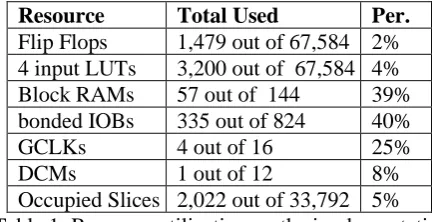
The development of these blocks has been accomplished using Celoxica's DK3 design suite and Xilinx ISE 7.1i place and route (PAR) tool. The hardware platform is composed of a Xilinx Virtex II XC2V6000 FPGA, with equivalent of 6 million logic gates and 2,592KB of dual-port BlockRAM [14]. This FPGA has been packaged with 4 banks (36-bit addressable) of external ZBT SRAM totalling 32Mbytes on the RC300 [4]. Table 1 is a summary of the resource utilization of the hardware implementation, using device xc2v6000, and package ff1152 and speed grade 6. The system is clocked at 25.17MHz and hence the pipeline yields approximately 25 MPixels/sec.
Resource Total Used Per.
[image:7.595.314.534.551.662.2]Flip Flops 1,479 out of 67,584 2% 4 input LUTs 3,200 out of 67,584 4% Block RAMs 57 out of 144 39% bonded IOBs 335 out of 824 40% GCLKs 4 out of 16 25% DCMs 1 out of 12 8% Occupied Slices 2,022 out of 33,792 5% Table 1: Resource utilization on the implementation
5 Experimental Results
and outdoor scenes. For this test we use eight different sequences; four indoor scenes and four outdoor scenes. The second test is to establish, which of the two algorithms can model perfectly a multimodal background. We use two sequences each with swaying trees, slow-moving objects and waving river.
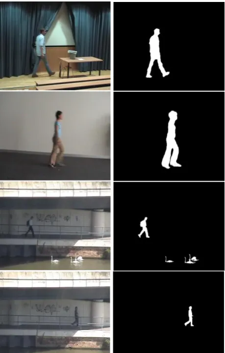
The experiments were conducted using MATLAB [25] as the development tool for K=3, 4 and 5 for both algorithms. For fair sensitivity comparisons, we use a learning rate of =0.2 for Grimson’s algorithm and T=0.7 as the threshold weight that account for the background. Similarly we use set T=7*K for our implementation, where K is the total number of clusters. We have constructed reference standard segmentations on these sequences by using manually marked frames; results of the algorithms are compared to this reference standard. Fig. 1 shows some sample frames of the sequences and their corresponding manually marked frames. We report pixel-wise errors against the reference standard, in terms of true positive (TP), true negative (TN), false negative (FN) and false positive (FP) pixels. Table 2 shows the sensitivity (SENS.) and specificity (SPEC.) of Grimson and GW4, for K=3. The test is conducted on a total of 340 frames, 170 frames from four different outdoor scenes and 170 frames from four different indoor scenes.
Fig. 1: Sample images with manually mark-out frames.
Scene
GW4 (%) Grimson’s (%) SENS. SPEC. SENS. SPEC. Out1 60.9 94.1 55.8 97.1 Out2 85.5 93.5 81.0 96.8 Out3 90.5 85.9 88.2 94.6 Out4 83.7 81.6 76.4 90.0 In1 81.1 89.5 76.9 93.1 In2 80.6 93.9 77.2 95.1 In3 87.3 95.0 85.1 97.0 In4 91.0 80.4 89.6 86.2
Table 2: Sensitivity and Specificity of GW4 against Grimson’s algorithm.
The evaluation parameters used are defined as follows:
FN TP
TP SENS
y Sensitivit
+ = .) (
FP TN
TN SPEC
y Specificit
+ = .) (
Table 2 clearly indicates the superiority of our algorithm in detecting foreground pixels (higher sensitivity than Grimson) in all 8 sequences and hence suitable for our target application. Figure 2, shows some outputs of the two algorithms after morphological opening for K=3.
[image:8.595.318.563.68.228.2] [image:8.595.309.542.381.740.2] [image:8.595.15.245.387.747.2]Our algorithm sometimes produce more false positive errors; this is a side-effect of the sensitivity of the model in detecting moving targets with low contrast against the background, which may lead to detection of the shadows of moving targets which Grimson's algorithm would ignore. Nonetheless, overall the error rate is lower than Grimson's [12]. Again, most of the noise produced in our approach can easily be removed with morphological opening at very minimal cost.
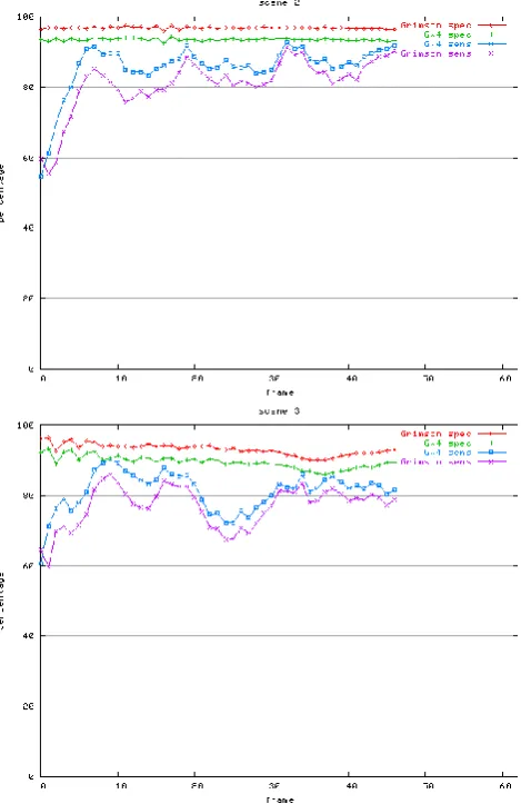
To show that this result is statistically significant we combine the results of all eight sequences for a sensitivity test. A binomial test is then conducted to test the null-hypothesis that the probability of Grimson’s algorithm performing better is greater or equal to 0.5. For p=0.5, since Grimson’s algorithm lost in all 8 independent scenes, the probability of performing better is (0.5)8=0.00390625 and hence reject the null hypothesis with 99% significance. The performance of one algorithm over the other is consistent for all frames in any particular sequence. Figure 3 shows how the sensitivity and specificity changes across frames for two selected scenes, when k=3.
Fig. 3: Graphs showing the sensitivity and specificity of the two algorithms for two independent sequences.
It is worth noting that Grimson's algorithm [12] although more sophisticated than ours, failed to perform better with the test data presented here, for K=3. This is due to the additional condition (condition 3) we use in extracting foreground pixels, thereby resolving the foreground aperture problem. From fig. 2, it becomes clear where Grimson's algorithm fails to perform better than GW4 due to foreground aperture. Further test were also conducted to evaluate the quality of results for both algorithms, when K increases. However, test results using the above 8 sequences did not show any significant improvement in sensitivity and specificity for K=4 and K=5 for both algorithms. Table 3 shows the average specificity and sensitivity for all 8 sequences with different values of K.
GW4 (avg. %) Grimson (avg. %) K SENS. SPEC. SENS. SPEC. 3 82.6 89.2 78.8 93.7 4 81.9 89.0 78.3 93.7 5 82.1 88.8 77.6 93.8
Table 3: Average sensitivity and specificity values for different values of K.
It will be unfair to judge the performance of our approach only on extracting moving objects. Hence, we perform test on two scenes with only slowly moving objects, swaying tress and waving river. This test is aimed at finding which of the two approaches best models a multimodal background. Fig. 4 shows some of the frames from the two sequences used in this test. Our interest here is the total number of true negatives for each algorithm. Table 4 shows the score for the two algorithms in terms true negatives and the number of frames an algorithm performs better than the other.
[image:9.595.329.555.261.329.2] [image:9.595.18.253.354.716.2] [image:9.595.310.564.501.702.2]
[image:10.595.309.561.68.368.2]
Normal Scene - frames 10, 150, 160 and 300 Fig. 4: Sequences for multimodal background test.
GW4 Grimson K TN (%) frames TN (%) frames 3 54.85 171 54.26 129 4 54.10 91 55.30 209 5 53.60 54 55.90 247 (a) Result for complex scene
GW4 Grimson K TN (%) frames TN (%) frames 3 69.60 300 67.10 0 4 68.80 204 67.80 96 5 68.30 153 68.30 147 (b) Results for normal scene
Table 4: Results of the multimodal modelling test for two scenes.
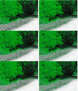
In general the performance of Grimson’s algorithm in modelling multimodal background improves as the value of K increases. The normal scene has a significant portion of static background, which accounts for the high performance with our implementation. It is also clear that GW4 performs better for lower values of K and hence the FPGA implementation with K=3 is better than Grimson’s algorithm for the same value of K. It is also worth noting that the complexity and storage requirement of the implementation increases while the value of K increases; making it impractical for FPGA implementation for speedup. Fig. 5 shows some results of the multimodal modelling for the complex scene while fig. 6 shows some results for the normal scene. Green pixels represent pixels that failed to be classified as background.
Fig. 5: Result of the complex scene for GW4 (left) and Grimson (right); for K =3, 4 and 5 respectively at frame 180/300.
[image:10.595.17.266.68.268.2] [image:10.595.46.257.319.485.2] [image:10.595.310.562.419.715.2]From table 3, GW4 always has lower specificity as compared to Grimson's algorithm due to GW4's sensitivity in detecting targets with low contrast to the background as well as reflections from moving objects. Clearly any form of error is undesirable. However, in our target application false positive (FP) errors of the type reported are more acceptable than false negative (FN) errors, as subsystem tracking stages can discard distracters such as shadows.
Timing analysis generated by the Place and Route (PAR) tool shows that the design can run at a maximum speed of 39.72ns, meaning every stage in the design can be clocked at 25.17MHz. Hence for a standard frame size of 640x480, the design can process at least 80fps (ignoring access to external RAM), when the pipeline is full. Comparing to real-time application requirement of 30fps, the implemented design, as it stands, meets the real-timing requirement. The efficient resource utilization of our design makes it possible to add new image processing functions, like object tracking and action interpretation to the system.
6 Conclusion
In this article we have shown a real-time adaptive background scene modelling and maintenance technique suitable for tracking people in both indoor and outdoor environments, implemented as a System-on-Chip (SoC) using FPGA technology.
Instead of using a complicated already existing background subtraction technique, our algorithm is a hybrid version of the W4 [8] and Grimson's [12] techniques, with
some modification to enhance the sensitivity in detecting targets with low contrast against the background. The system learns and models the background scene over time to detect foreground objects, in the presence of multimodal background objects like tree branches. The algorithm has been implemented in Handel-C and runs on Xilinx Virtex II FPGA. Currently, for an image size of 640x480, the system operates at real-time (30fps). This performance level cannot be easily reached without parallel processing. Various tests have also been conducted using MATLAB to justify the performance of our approach. Generally, our results show that our implementation is optimal for the available FPGA resources.
References:
[1] AccelChip, Comparison of Methods for Implementing DSP Algorithms, SoC Central, 2003
[2] Elham Ashari and Richard Hornsey, FPGA implementation of real-time adaptive image thresholding, SPIE-International Society for Optical Engineering, Dec. 2004.
[3] J. Batlle, J. Martin, P. Ridao and J. Amat, A New FPGA/DSP-Based Parallel Architecture for Real-Time Image Processing, Elsevier Science Ltd., 2002
[4] Celoxica, Video and Imaging solution, http://www.celoxica.com, 2004.
[5] M. Ekinci and E. Gedikli, Real Time Background model initialization and maintenance for video surveillance, IJCI Proceedings of Intl. XII.Turkish Symposium on Artificial Intelligence and Neural Networks, 2003
[6] Ahmed Elgammel, David Harwood, and Larry Davis, Non-parametric Model for Background Subtraction, Proceedings of the 6th European Conference on Computer Vision, Dublin, Ireland, 2000
[7] D. Gutchess, M. Trajkovic, E. Cohen-Solal, D. Lyons and K. Jain, A Background Model Initialization Algorithm for video Surveillance, IEEE, International Conference on Computer Vision, 2001.
[8] I. Haritaoglu, D. Harwood and L. Davis, W4: Who?
When? Where? What? A real time system for detecting and tracking people, IEEE Third International Conference on Automatic Face and Gesture, 1998
[9] Hongtu Jiang and Viktor Owall, Controller Synthesis in Hardware Accelerator Design for Video Segmentation, SSoCC, 2004.
[10] K. Johnston, D. Gribbon and D. Bailey, Implementing mage Processing Algorithms on FPGAs, Proceedings of the Eleventh Electronics New Zealand Conference, Palmerston North, Nov. 2004.
[11]Craig Sanderson and Dave Shad, FPGAs Supplant Processors and ASICs in Advanced Imaging Applications, FPGA and Programmable Logic Journal, 2005.
[12] C. Stauffer and W. E. L. Grimson, Adaptive background mixture models for real-time tracking, IEEE Conference on Computer Vision and Pattern Recognition, 1999. [13] C. Wren, A. Azarbayejani, T. Darrel and A. Pentland,
Pfinder: Real-time tracking of human body, IEEE Transactions on Pattern Analysis and Machine Intelligence, 1997.
[14]Inc. Xilinx, Virtex II Platform Field Programmable Gate
Arrays Data sheet,
http://direct.xilinx.com/bvdocs/publications, March 2005. [15]Pavel Zemeik, Hardware Acceleration of Graphics and Imaging Algorithms using FPGAs. Proceedings of Spring Conference on Computer Graphics, 2002.
[16]I. Haritaoglu, D. Harwood and L. S. Davis, W4: Real-Time Surveillance of People and Their Activities. IEEE Transactions on Pattern analysis and machine intelligence, Vol.22, No.8, August 2000.
[17]Qi Zang and Reinhard Klette, Robust Background Subtraction and Maintenance, Proceedings of the 17th IEEE International Conference on Pattern Recognition (ICPR’04), 2004.
[19]C. Stauffer and W. E. L. Grimson, Learning Patterns of Activity Using Real-Time Tracking, IEEE Transactions on Pattern Analysis and machine intelligence, Vol.22, No.8, August 2000.
[20]A.Monnet, A. Mittal, N. Paragios and V. Ramesh, Background Modeling and Subtraction of Dynamic Scenes, Proceedings of the 9th IEEE International Conference on Computer Vision, 2003.
[21]S. Jorg, J. Langwald and M. Nickl, FPGA based Real-Time Visual Servoing, Proceedings of the 17th IEEE International Conference on Pattern Recognition, 2004. [22]A. Mittal and N. Paragios, Motion-Based Background
Subtracting using Adaptive Kernel Density Estimation, Proceedings of the IEEE Computer Society Conference on Computer Vision and Pattern Recognition, 2004. [23]R. Matousek, M. Danek, Z. Pohl, R. Bartosinski and Per
Honzik, Reconfigurable System-on-a-Chip, The Syndicated: A Technical Newsletter for ASIC and FPGA Designers, July 2005.
[24]M. Mason and Z. Duric, Using Histograms to Detect and Track Objects in Color Video, Proceeding of the 30th IEEE Applied Imagery Pattern recognition Workshop, 2001.
[24]http://www.mathworks.com/
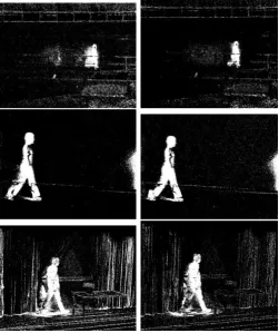
Fig. 7: Raw outputs of the two algorithms without morphological opening for K=3 for three different scenes. GW4- left and Grimson’s algorithm – right.
Fig. 8: Raw outputs of the two algorithms without morphological opening for K=4 for three different scenes. GW4- left and Grimson’s algorithm – right.
[image:12.595.310.563.70.365.2] [image:12.595.17.269.383.681.2] [image:12.595.312.564.418.718.2]