LEABHARLANN CHOLAISTE NA TRIONOIDE, BAILE ATHA CLIATH TRINITY COLLEGE LIBRARY DUBLIN OUscoil Atha Cliath The University of Dublin
Terms and Conditions of Use of Digitised Theses from Trinity College Library Dublin
Copyright statement
All material supplied by Trinity College Library is protected by copyright (under the Copyright and Related Rights Act, 2000 as amended) and other relevant Intellectual Property Rights. By accessing and using a Digitised Thesis from Trinity College Library you acknowledge that all Intellectual Property Rights in any Works supplied are the sole and exclusive property of the copyright and/or other I PR holder. Specific copyright holders may not be explicitly identified. Use of materials from other sources within a thesis should not be construed as a claim over them.
A non-exclusive, non-transferable licence is hereby granted to those using or reproducing, in whole or in part, the material for valid purposes, providing the copyright owners are acknowledged using the normal conventions. Where specific permission to use material is required, this is identified and such permission must be sought from the copyright holder or agency cited.
Liability statement
By using a Digitised Thesis, I accept that Trinity College Dublin bears no legal responsibility for the accuracy, legality or comprehensiveness of materials contained within the thesis, and that Trinity College Dublin accepts no liability for indirect, consequential, or incidental, damages or losses arising from use of the thesis for whatever reason. Information located in a thesis may be subject to specific use constraints, details of which may not be explicitly described. It is the responsibility of potential and actual users to be aware of such constraints and to abide by them. By making use of material from a digitised thesis, you accept these copyright and disclaimer provisions. Where it is brought to the attention of Trinity College Library that there may be a breach of copyright or other restraint, it is the policy to withdraw or take down access to a thesis while the issue is being resolved.
Access Agreement
By using a Digitised Thesis from Trinity College Library you are bound by the following Terms & Conditions. Please read them carefully.
Analysis of noise source mechanisms for
a subsonic jet
O
r l aP
o w e rA thesis su bm itted to th e University of D ubhn in partial fulfilment of the requirem ents for the degree of Ph.D .
D epartm ent of Mechanical & M anufacturing Engineering, University of D ublin,Trinity College, Dublin, Ireland.
■^TRINITY C O LLEG ^^i 1 0 NCV
D eclaration
1 declare th a t this thesis has not been subm itted for a degree a t this or any other university and th a t any works carried out are rny own unless otherw ise referenced. In addition, 1 grant permission to th e T rinity College D ublin Library to lend or copy this thesis upon request.
A b stract
D espite advances in engine design, from higli bypass to co-axial or lobe shaped nozzles, th e problem of jet noise reduction continues to require ongoing research in order to comply w ith th e criteria inherent in envirom nental objectives set out by relevant bodies worldwide. F undam ental to this work, will be a clearer understanding of th e generation and propagation of noise sources in subsonic jets.
In this regard, it is the aim of this thesis to identify and exam ine noise source mechanisms from a subsonic jet. The correlation between the velocity fluctuations inside the jet and th e near-field acoustic pressure is m easured and a m ultiple inj)ut / m ultiple o u tp u t model is im plem ented. This identifies how each source, independent of all others, propagates and radiates into th e near-field. T hrough the use of dedicated testing, specifically designed to extract inform ation on source propagation, techniques such as those proposed in this work will lead to further understanding of how source term s behave in a subsonic jet.
For this purpose Laser Dopi)ler A nem om etry has proved to be an extrem ely useful technique since it enables very complex flow conditions to be m easured successfully. L iteratu re shows th a t the random acquisition of d a ta associated w ith this technique has received considerable atten tio n , w ith many m ethods available to process the random data.
A cknow ledgem ents
E V E R Y E N G I N E E R . . . .
Every little engineer needs a John Fitzpatrick for guidance, encouragement and support, thanks John.
Every engineer can’t survive without other engineers - we feed off eacfi other, some of us quite literally!!
for all those entertaining highs and lows, thanks to all....
E very engineer works in a group - its better for socialising!!
thanks to Craig Meskell, the Fhiids & Vibration group, can’t forget those Thermo guys either!
E very engineer needs a m athematician (thanks for the ‘Welcome to ^ ’) if any mistakes are present we know who to blame!
Every engineer also needs a non-engineer, who doesn’t want to hear about jet noise all day long!!
thanks for keeping my sanity...
C ontents
1 I n tr o d u c tio n 1
1.1 O b jectiv es & O v i t li u e ... 3
2 J e t N o is e 5 2.1 T u rb u len t S hear F l o w s ... fi 2.2 Sources of N o i s e ... 7
2.3 T urb u len ce s t r u c t u r e s ... 9
2.4 Noise P a t t e r n ... 10
2.5 R ecent D evelopm ents in J e t Noise R esearch ... 13
2.6 M odelling & P re d ic tio n of J e t N o i s e ... K) 2.6.1 A e r o d y n a m ic s ... 16
2.6.2 Som ce an d P ro p a g a tio n P r e d ic tio n s ... 17
2.7 S u m m ary ... 18
3 L D A P r o c e ssin g T ech n iq u es 20 3.1 Sam ple k , H o l d ... 21
3.1.1 N on-coincident LDA S i g n a l s ... 24
3.1.2 C oincident LDA S i g n a l s ... 26
3.1.3 O ne LDA Signal & a C onventional I n s t r u m e n t ... 27
3.2 Slot C o r r e l a t i o n ... 28
3.3 C oncluding R e m a r k s ... 31
4 P r e lim in a r y A n a ly s is o f L D A D a ta 32 4.1 Sam ple k . Hold A n a l y s i s ... 32
C O N T E X T S C O N T E N T S
4.2.1 M e a su re m e n ts ... 35
4.2.2 Auto S p e c t r a ... 39
4.2.3 Cross S p e c t r a ... 41
4.2.4 Coherence & P h a s e ... 42
4.2.5 Cross C o r r e la tio n ... 45
4.2.6 Convection V elo city ... 46
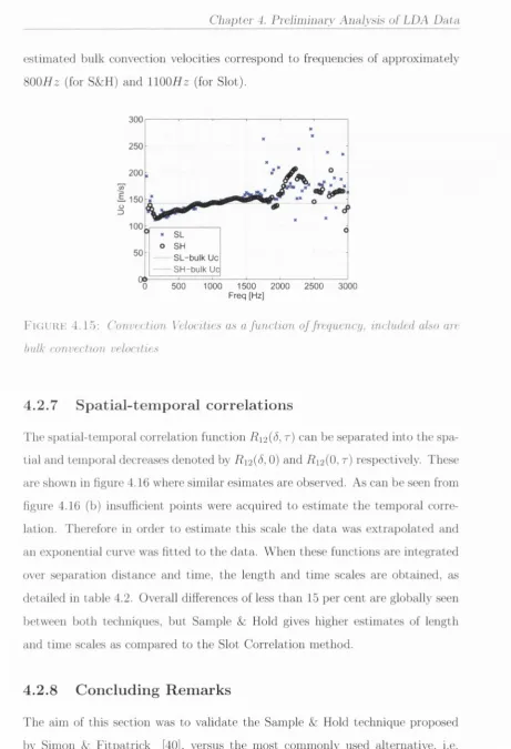
4.2.7 Spatial-tem poral c o rrelatio n s... 48
4.2.8 Concluding R e m a r k s ... 48
4.3 LDA acquisition m o d e s ... 50
4.3.1 Velocity F lu c tu a tio n s ... 51
4.3.2 Reynolds Stress T e r m s ... 53
4.3.3 Coherence e s t i m a t e s ... 58
4.3.4 Concluding R e m a r k s ... 62
5 A c o u stic E x p e r im e n ta l A n a ly sis 63 5.1 Configuration 1 ( r / D = 1 . 1 ) ... 68
5.1.1 Auto S p e c t r a ... 68
5.1.2 C o h e re n c e ... 70
5.1.3 Phase ... 75
5.2 Configuration 2 { r / D = 4 . 5 ) ... 78
5.2.1 Auto spectra ... 79
5.2.2 C o h e re n c e ... 83
5.2.3 Phase ... 86
5.3 Concluding R e m a r k s ... 88
6 S o u rce Id e n tific a tio n 91 6.1 Five Input M o d e l ... 92
6.2 E xperim ental S e t u p ... 94
6.3 R e s u lts ... 95
6.3.1 Configuration 1 ... 98
C O y r E N T S C O N T E N T S
List o f Figures
2.1 S tru c tu re of a J e t ... 6
2.2 L on g itu d in al an d L a tera l Q u a d r u p o l e s ... 8
2.3 C onvection & R e f r a c t i o n ... 10
2.4 C one of S i l e n c e ... 11
2.5 G eo m etry for q u a d ru p o le c o r r e la t io n s ... 12
2.6 J e t Noise P a t t e r n ... 13
2.7 kR d e m a rca tio n at lO O O H z... 15
3.1 Sam ple &: Hold: R e-sam pling a ran d o m acquired LDA signal a t equal tim e i n t e r v a l s ... 21
3.2 S chem atic of th e Sam ple k. Hold P ro ced u re ... 22
3.3 S chem atic of Tw o LDA s ig n a l s ... 25
3.4 S chem atic of an LDA signal an d a conventional in stru m e n t (e.g. hot-w ire or m i c r o p h o n e ) ... 27
3.5 T h e w eighting schem e of th e fuzzy s lo ttin g t e c h n i q u e ... 30
4.1 S am ple & Hold F ilte rs (a) C o n tin u o u s {h) D is c r e te ... 33
4.2 A u to S p ectral e stim a tio n illu stra tin g th e Sam ple & Hold correction s 34 4.3 Noise to Signal R a t i o ... 34
4.4 C lose-up of th e JE A N n o z z le ... 3(i 4.5 O ne point / two com ponen t m easu rem en ts perform ed a t C E A T P oitiers, F rance under th e JE A N c o n tra ct ... 37 4.6 A xial d istrib u tio n of th e m ean velocity com po nents (m easu rem en ts
L I S T O F F I G U R E S L I S T O F F I G U R E S
4.7 R ad ial d istrib u tio n of th e m ean velocity com p o n en ts (m e a su re m en ts perform ed a t C E A T P o itiers, F rance u n d e r th e JE A N con tra c t) ... 39 4.8 L ocation of JE A N tw o -p o in t m easu rem en ts on J e t 3 ... 40 4.9 A u to s p e c tra of u': C o m p ariso n of S am ple & Hold a n d Slot C or
rela tio n e s t i m a t e s 40
4.10 C ross sp e c tru m of u[ & U2- C o m parison of S am ple & H old a n d Slot C o rrela tio n e s t i m a t e s ... 41 4.11 C oherence e stim a te s from th e tw o -p o in t m easu rem en ts : c o m p a ri
son of Sam ple & Hold a n d Slot C o r r e l a ti o n 43 4.12 P h a se estim ates: com parison of S am ple k. Hold a n d Slot C o rre la tio n 44 4.13 C ross C o rrela tio n e stim a te s using S am ple & Hold an d Slot C o rre
latio n ... 46 4.14 C o n to u r C o rrela tio n C urves from tw o-point / o ne-com ponent m ea
su re m e n ts (a) Sam ple & Hold, (b) Slot C o rrela tio n ... 47 4.15 C onvection V elocities as a fu n ctio n of f r e q u e n c y ... 48 4.16 S p a tia l an d T em p o ral C o rrela tio n functions co m paring S am ple &
Hold a n d Slot C o r r e l a t i o n ... 49 4.17 A u to S p e c tru m of u' : C o m parison betw een C oincident and N on
coincident m o d e s ... 52 4.18 Noise to Signal R a tio of u ’ : C o m parison betw een C oincident an d
N on-coincident m odes ... 52 4.19 A u to S p e c tru m of v' : C o m parison betw een C oincident a n d N o n
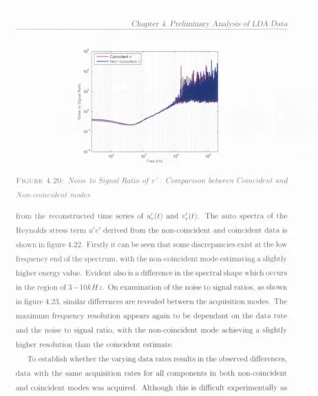
coincident m o d e s ... 53 4.20 Noise to Signal R a tio of v ’ : C o m parison betw een C oincident an d
N on-coincident m odes ... 54 4.21 C o m parison betw een C oincident an d N on-coincident m odes of th e
A u to S p e c tru m of (a) a n d (6) 55
L I S T OF F I G U R E S L I S T OF F I G U R E S
4.23 Noise to Signal R ations of u'v': Com parison between Coincident and N on-coincident m o d e s ... 5G 4.24 A uto Spectrum of u'v' (same d a ta rates) ; Comparison between
Coincident and Non-coincident m o d e s ... 57
4.25 Noise to Signal R ations of u'v' (same d a ta rates): Comparison between Coincident and Non-coincident m o d e s ... 57
4.26 U ncorrected Coherence and C orrected Coherence between the ve locity fluctuations and Reynolds s t r e s s e s ... 60
4.27 U ncorrected Coherence and C orrected Coherence between (a) u' k v', (b) u' & u'v' and (c) u'"^ & u'v' ... 61
5.1 Schem atic of experim ental s e t u p ... 64
5.2 T C D J e t ... (i4
5.3 Je t P r o f i l e ... 65
5.4 Schem atic of experim ental s e t u p ... 67
5.5 r / D = 1.1\ M icrophone A uto S p e c t r a ... 68
5.6 r / D = 1.1: Coherence - M icrophone 1 ... 69
5.7 r / D = 1.1: Microphone A uto S pectra C o n d itio n e d ... 70
5.8 r / D = 1.1: Microphone Coherence (effects of conditioning) . . . . 71
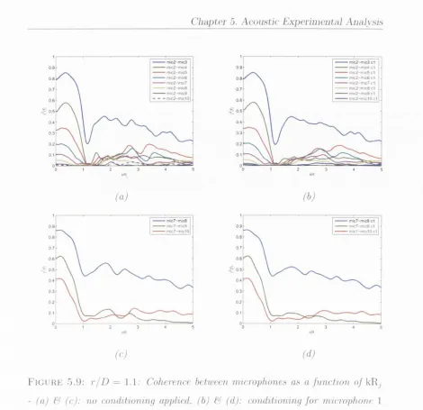
5.9 r / D = 1.1: M icrophone Coherence as a function of kRj (effects of conditioning) ... 72
5.10 r / D = 1.1: Microphone Coherence - p ro p a g a tio n ... 73
5.11 r / D = 1.1: C ontour Coherence ... 74
5.12 r / D = 1.1: C ontour Coherence c o n d itio n e d ... 75
5.13 r / D = 1.1: M icrophone P hase - f r e q u e n c y ... 76
5.14 r / D = 1.1: M icrophone P hase - k R j... 77
5.15 r / D = l.\-. M icrophone Phase - p r o p a g a t io n ... 78
5.16 r / D = 1.1: Convection velocity as a function of frequency . . . . 78
5.17 r / D = 4.5: M icrophone A uto S p e c t r a ... 79
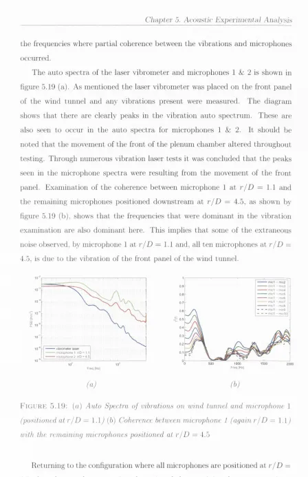
5.18 Coherence and Phase between vibrations and microphones . . . . 80
L I S T OF FI GURES L I S T OF FI G U R E S
5.20 r / D = 4.5; Coherence - M icrophone 1 ... 82
5.21 r / D = 4.5: M icrophone A uto S pectra C o n d itio n e d ... 82
5.22 r / D = 4.5: Coherence - M icrophone 2 ... 83
5.23 r / D = 4.5: M icrophone Coherence - p ro p a g a tio n ... 84
5.24 r / D = A.b\ C ontour Coherence ... 85
5.25 r / D = 4.5: C ontour Coherence c o n d itio n e d ... 86
5.26 r / D = 4.5: Microphone P h a s e ... 87
5.27 r/Z ) = 4.5: Microphone Phase - p r o p a g a t io n ... 88
6.1 Conditioned inputs k. o u t p u t s ... 93
6.2 Experim ental Setup at Trinity - combined LDA and acoustic mea surem ents ... 94
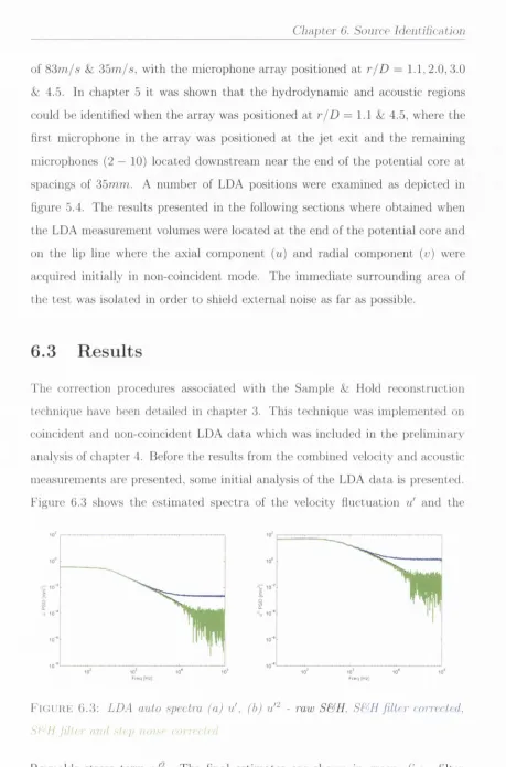
6.3 LDA au to sp ectra - u ... 95
6.4 LDA au to sp ectra - v ... 96
6.5 LDA cross spectra ... 96
6.6 Corrected Coherence between LDA s o u r c e s ... 97
6.7 r / D = 1.1: O rdinary Coherence between LDA sources and micro phones 99
6.8 r / D = 1.1: P artial Coherence between LDA sources and micro phones 100
6.9 r / D = 1.1: P artial Coherence between LDA and m icrophones . . 103
6.10 r / D = \.l: M ultiple C o h e r e n c e ... 105
6.11 r/Z ) = 1.1: norm -I- 0-4k: Angle of Frequency Response Function . 105 6.12 r / D = 1.1: Angle of Frequency Response F u n c tio n ... 106
6.13 r / D = 1.1: Angle of Frequency Response Function - coincident d a ta l0 8 6.14 r / D = 4.5: O rdinary Coherence & C onditioned coherence - Veloc ity f l u c t u a t i o n s ... 109
6.15 r / D = 4.5: O rdinary Coherence & Conditioned coherence - Reynolds s tre s s e s ... 110 6.16 r / D = 4.5: P artial Coherence between LDA sources and micro
L I S T OF F I G U R E S L I S T OF F I G U R E S
List o f Tables
4.1 JEA N tem p eratu re and velocity in f o r m a tio n ... 37 4.2 Length & Tim e Scales and Convection velocity estim ates using
Sample & Hold and Slot C orrelation ... 49 4.3 D ata rates and Re-sample rates for non-coincident and coincident
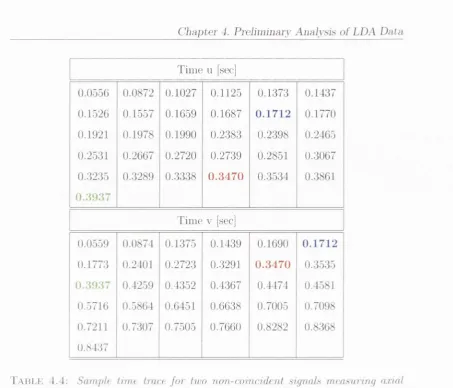
m o d e s ... 51 4.4 Sample tim e trace for two non-coincident signals measuring axial
and radial v elo cities... 58
N om enclature &: A bbreviations
a
S
e
Noise to Signal R a tio C oherence
D isplacem ent angle to jet axis variance
P hase
C o C o rrected D oppler am plification factor D D iam eter of je t
dt tim e step / frequency /„, m ean d a ta ra te
f r R e-sam ple ra te G { f ) O ne sided sp e c tru m
k W avenum ber
! ( / ) filter
/? R adial d ista n c e
Bj R ad ial d ista n c e from sh ear layer axis to th e second m easu rem en t p o sitio n (j) H{S, t) C o rrela tio n C urve
T\ Taylor micro-scale
t Time
u Velocity vector u Mean velocity w Velocity fluctation
Reynolds stress term Convection Velocity R econstructed tim e series Reynolds stress term Jet exit velocity Reynolds stress term x{t) Tim e signal
X ( f ) Fourier transform
X* { f ) C onjugate of Fourier transform
x / D Axial distance normalised by th e diam eter Uc
Ki t )
u'v'
Un
CFD C om p utatio nal F luid D ynam ics DNS D irect N um erical Sim ulation FP'T F ast F ourier T ransform HWA H o t-W ire A neniom etry
JEAN J e t E xhaust A erodynam ic Noise LDA Laser-D oppler A neniom etry LEE Linearised E uler E quations LES Large E d d y Sim ulation PSD Pow er S pectral D ensity
C hapter 1
In trod u ction
Aeroacoiistics is a discipline th a t unites such topics as acoustics, fluid mechanics, flow induced sound, and flow induced vibration. It is a m ultidisciplinary subject th a t has been slow to gain acknowledgment, particularly in engineering where it is essent ial to deal with problem s related to envirom nental noise. There is a need to reduce noise and vibration due to aeroacoustic phenom ena, but at the same time, th a t has regard to th e effect on perform ance and cost. In th e aeroplane industry, in this regard, it is particularly im portant to minimize the effects of any alterations or modifications to aircraft th a t would result in significant increases in dim ensions and weight.
Chapter 1. Inlrodnciion
‘ringing’ in th e ear. Extensive dam age to th e nerves and sharp pain will occur w ith levels in th e region of lAOdB. T he m ost serious dam age, resulting in mass destruction of the auditory nerves w ith a persistent ringing in the ears, occurs at levels of 150 — 160dB. The noise levels in the vicinity of aircraft reach these dangerous levels of IGOdB.
At m ajor airports around th e world, including Dublin airport, legislation ex ists to lim it the effect of noise in th e surrounding areas. These m easures require restrictions on m aintaining certain flight path s im m ediately following takeoff, prioritisation of ruiw ays for noise abatem ent purposes and avoidance of reverse th ru st procedures on landing specifically between th e hours of l l p rn and 6am. Presently Dublin airpo rt m onitors noise levels using a Briiel & K jaer system which consists of six fixed statio ns positioned around the airport in addition to two mobile units.
T he aviation industry continues to experience significant growth w'ith forecasts suggesting a dem and for 7600 new aircraft every decade, representing a m arket investm ent of 1300 Ijillion euro by 2019. In the three decades since aviation became an environm ental issue, there have been significant im provem ents in noise abatem ent. For example, the noise footprint of an A irbus A320 is 80 per cent smaller th a n an older Boeing 727-200. The noise level of an A irbus A320 is approxim ately 20dB less th a n th a t of a Caravelle or Boeing 727 of 40 years ago. As reported by Ffowcs-Williams [2] th e first generation Boeing 707 at take-off produced as nuich somid as the world population shouting in phase! A Boeing 767 of 30 years later (w ith four tim es as much th ru st per engine) produced as much sound as the city of New York shouting in phase. D espite these advances the A eronautics and Space T ran spo rtation Technology Enterprise of NASA has set 25 Year Deliverables to achieve 20dB com m unity noise im pact reduction relative to 1997 levels.
C h a p te r 1. In tro d u c tio n
high bypass ratio, low je t efflux velocity engines has brought about other sources, referred to as excess noise, tailpipe noise, or core noise. High bypass ratio engines have led to a reduction in aircraft noise, although this is a direct result of the lowered velocity com pared to the low bypass engines. W hile th e com bined noise produced by a je t engine m ay be dom inated by fan noise, th e je t exhaust is still the most dom inant source at full power. W ith ou t significant im provem ents in technology the m axim um bypass ratio is lim ited by m any factors, for exam ple rotor speed and length of fan blades, and currently m odern engines operate at near this m axinnm i value. Therefore the procedure of increasing the bypass ratio to reduce the je t noise is limited.
1.1
O bjectives
Sz. Outline
Previous experim ental work into the origin of je t noise has used statistic al m eth ods to obtain inform ation on noise sources. These techniques have resulted in the atx'uniulatioii of useful inform ation regarding the average noise source location but have failed to provide detailed inform ation regarding the noise generation mechanisms. Consequently it will be necessary to develop new techniques th a t will result in je t noise reduction in the long term . This w'ill entail a clearer and more thorough m iderstanding of the source m echanisms and will evolve only if reliable m ethods for modelling these mechanisms can be developed.
T he latest developments in com putational fluid dynam ics (CFD) provide in form ation on the statistical character of the flow field and also on its instantaneous behaviour. This is used to build prediction techniques beised on an understanding of the noise generation mechanisms. The focus of this present work therefore is to exam ine experim entally the relationship between turb ulent stru ctu res in the jet and the associated noise generation mechanisms, as this has not received adequate atten tio n to date.
C h a p te r 1. lntix>duction
C hapter 2
J et N oise
Ch<ij)tcr 2. Jet ?^oisc
2.1
T urbu len t Shear F low s
An exam ple of a free shear flow is the je t formed when fluid is continuously added to an otherw ise stag nan t fluid. The area separating th e turbulent jet from the surrounding am bient flow is random in shape and continuously changing. T he movement of this interface induces rotation al fluid m otion of the surrounding fluid.
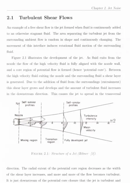
Figure 2.1 illustrates th e developm ent of the jet. As fluid exits from th e nozzle the flow of th e high velocity fluid is fully aligned w ith the nozzle wall, and a core region of po ten tial flow is formed (hence ‘potential core’). Between the high velocity fluid exiting th e nozzle and the surrounding fluid a shear layer is generated. Due to the addition of fluid from th e surroundings (entrainm ent) this shear layer grows and develops and th e am ount of tu rb u len t fluid increases in th e dow nstream direction. This causes the je t to spread in th e transversal
S e l f - s i m i lor p r o f i l e s
N o z z l e T u r b u l e n c e
I n t e n s i f y
y , / D
M e o n v e l o c i t y
I
T r a n s i t i o n I r e g i o nMix ing r e g i o n Fully d e v e l o p e d j e t
FlGlJHti 2. f ; Struclure of a JeL {Rihner [3j)
[image:25.533.50.499.37.669.2]C h c i j ) l c r 2. J e t N o i s e
Fully developed turbulence is a turbulence which is free to develop w ithout imposed constraints. The possible constraints are boundaries, external forces, or viscosity. Im plying th a t no real turbulen t flow, can be fully developed in th e large energetic scales, even at high Reynolds numbers. At smaller scales, turbulence will be fully developed if the viscosity does not play a direct role in th e dynam ics of tliese scales. However for theoretical purposes, when studying a freely-evolving statistically homogeneous turbulence, it is possible to assume th a t turbulence is fully developed in bo th the large and small scales.
Self-sirnilar profiles are observed in this far field where the m ean velocity [)rofiles experience a linear grow th of the je t w idth and a linear decay of the square of centerline velocity. T he assum ption th a t these self-sim ilarity profiles are independent of initial conditions for all quantities and are therefore stan d ard for all jets has been cjuestioned by George [4]. The mean velocity profiles become self-preserving about 5 diam eters dow nstream . D etails of the tu rb u len t stru ctu re can take much longer to become self-similar.
2.2
Sou rces o f N o ise
It was not until the 1950’s when Lighthill [5] developed a general theory of aerodynam ic sound generation, which becam e known as the Lighthill Acoustic Analogy Theory, th a t Jet Noise becam e a significant issue. In his theory, Lighthill proposed th a t the unsteady tu rbu lent fluctuations which give rise to noise are replaced by a volume d istribution of equivalent acoustic sources em bedded in an otherwise luiiform m edium at rest. The propagation of sound in a uniform m edium is governed by th e equations
Chapter 2. Jet Noise
waves. The result is an inhomogeneous wave equation of th e form:
(2.1) where p is the density, is th e am bient sound speed, and
Ty = pvivj + { p - + Tij (2.2)
is know'n as the Lighthill stress tensor, where Vi, p, and are th e velocity, pressure, and viscous tensor stresses and 5ij is th e Kronecker delta. The left hand side of equation 2.1 represents acoustic wave propagation and the right hand side the sources th a t generate th e noise field. These source term s involve second spatial derivatives of th e stress tensor and are referred to as quadrupoles, depicted in figure 2.2. Physically the quadrupole strength is equivalent to the
applied stress to an element of fluid suffering from equal and opposite forces. W here each source of th e applied stress is equivalent to a dipole and each such pair to a quadrupole. The au to correlation of the acoustic pressure, in term s of the correlation function of the Lighthill tensor is given by equation 2.3, where the Doppler correction factor (Co) i» applied.
Stress Stress Ti2
Quadrupole equivalent
Chciplcr 2. Jet Noise
A very im portant result came from Lighthill’s inhomogeneous wave equation. By using a Green’s function for the wave equation, Lighthill estabhshed th at the acoustic power radiated by a jet should vary as the eighth power of the jet velocity. This agreed with available experimental d ata and became known as the
\ f
Law.2.3
T urbu len ce stru ctu res
Knowledge of the characteristics of jet flow's is essential to the understanding of .Jet Noise since the sources of sound are defined by the turbulence struct ures. In the f950’s, turbulence was considered to be a random assortment of small eddies. As a consequence, the primary focus of jet noise investigation at th at time was to quantify the noise generated from fine-scale turbulence, as reviewed by Tam [6]. Later Crow
L
Champagne [7], and Brown & Roshko [8] discovered independently the existence and importance of large-scale, as well as fine-scale structures within turbulence in jets and mixing layers. It was found th at these large-scale structures were im portant noise sources for supersonic jets. However at th at time their importance in subsonic jets was not established. It was not until 1998 th at Tam [6] showed th a t both large and fine-scale structures are responsible for the noise th at is generated in subsonic jets.C hapter 2. Jet Noise
2.4
N o ise P a tte r n
T he souiid generating structu res or quadrupoles in jet flows are convected down stream by the m ean flow, so th a t the sources are moving. Lighthill realised the im portance th a t the source convection effect has on th e directivity of je t noise, which is more obvious a t higher je t velocity. Ffowcs-Williams [11] found th a t, by extending Lighthill’s dim ensional argum ent including th e effect of source convec tion, for high speed je ts the power of the rad iated noise should vary as the third power of the je t velocity, i.e. P ~ Tam [6] and R ibner [12] showed th a t moving sources tend to rad iate more sound in th e direction of m otion. W hen quadrupoles generate sound, in order to reach th e far field, this sound m ust prop agate through th e je t flow. As th e m ean flow' is highly non-uniform the sound is refracted as it travels outw ard from the je t How' resulting in less sound being rad iated in the direction of the flow, as shown in figure 2.3. This effect creates a relatively quiet region surrounding th e je t axis - known as th e cone of silence (see figure 2.4). Atvars et al [13] dem onstrated experim entally th a t the noise intensity drops by more th a n 2QdB due to th e presence of th e cone of silence.
Refraction
Nozzle
Convection
Fk u'RE 2.3: Convection & Refraction
C h a p t e r 2. Jet N oise
Cone of Silence
> >
F i g u r e 2 . 4 ; Cone o f Silence
enables th e quadrupole velocity correlations contributing to th e generation of soiind to be exam ined, as was shown by Ribner [12], Source term s th a t contain only turbu lent velocity com ponents and th a t are independent of th e m ean flow
are defined as self noise. W hereas term s tliat contain both tu rb u len t velocity and m ean flow com ponents are known as shear noise. T he self noise term s have the form; uiujii'i^u'i while th e shear noise term s have th e form; UiU^UiUj. The quadrupole correlation can be expressed as a function of the m idpoint and th e separation in space and time, as show'u in figure 2.5. R ibner [12] analysed tlie potential contribution of th e source term s and concluded th a t only nine of
the thirty-six possible quadrupole correlations yield distinct contributions to the axisynnnetric noise p a tte rn of a round jet. T he correlations contribu te either cos^6*, cos^ 6^sin^ 6^, or sin“*0 directional pattern s, where 6 is th e angle w ith the je t axis. He showed th a t th e nine self-noise p attern s combine as:
The self noise is radiated equally in all directions whereas th e shear noise gives a dipole like contribution. Therefore the overall ‘basic’ p a tte rn is th e addition
/4cos** 6^(1) -I- Acos^ 0sin^ 0 ( | + g + | + | ) + Asin'* + ^ + ^ + ^ )
= A(cos'^ e + sin^ e f = A (2.4)
C l m p t c r 2. Jet N oisv
X i
Observer
Observer
Quadnipolc strength
pvivj
Quadrupole strength
pvWi
Fl Gi ' HK 2. 5 : Gvonie.lry f o r quadrupole correlations, (R'lbner [12])
of the self and shear noise term s, resulting in a form shown in equation 2.6 and illustrated in figure 2.6 as the basic p attern .
/I + B(cos^ 0 + cos^ ^^)/2 (2.6)
In addition to the basic p attern , th e directional p a tte rn of je t noise is dom inated by convection and refraction. Figure 2.3 also shows the effect of convection on the sound waves, where it atte m p ts to corivect sound waves dow nstream into a broad fan enveloping the jet. Convection and refraction alter th e basic noise p a tte rn of a jet to the form shown in figure 2.6, where th e resulting shape is a heart-shaped p a tte rn of jet noise.
radiat-Chciptcr 2. Jcl N o ise
- 3db
Self noise A
+
Shear noise B{cos*e + cos^e)l2
Basic pattern
Basic
(figure 2) Convection
(C"’ factor)
^
Jet RefractionF i g u r k 2 . G : Jet Noise P a tte rn (B ih n e r [12])
ing q u a d ru p o le s are th e fo u rth a n d second o rd er term s, co rresp o n d in g to self
an d shear noise m echanism s respectively. T h ro u g h single an d tw o -p o in t tu r b u
lence velocity m easu rem en ts an e stim a te of th e q u ad ru p o le field s tr u c tu r e can be
achieved. C onsidering only a two dim ensional slice th ro u g h th e je t th e necessary
required term s are: uiu'^, U2U2, u^u'^, u^u^-, u \ u2 i u i u2u \ u2
-2.5
R ec e n t D ev e lo p m en ts in J e t N o ise R esea rch
T h ro u g h o u t th e 1980’s th e frequency co n te n t of je t noise was m easu red in 1 /3
octave bands. However th is tech n iq u e artificially enhances th e im p o rta n c e of th e
high frequency noise com p o n en t, w hich co m plicated th e physical in te rp re ta tio n of
C l m p t e r 2. Jet N oise
in the following decade led to detailed analysis being carried out on the two
components of turbulent mixing noise in supersonic jets.
Hussain [10] showed th a t large eddies evolve and interact in three ways.
Firstly, structures form and convect downstream while growing in size. Secondly,
when a fast moving structure catches up with a slower structure th a t is further
downstream, they begin to rotate about a common point leading to ‘pairing’ of
the two structures. Thirdly, individual structures have been observed to break
dow'ii into two or more separate structures. The understanding of how these
structures behave is im portant in the understanding of turbulence and hence jet
noise.
Convection velocity is an im portant quantity in aeroacoustics since it can
be used to establish the speed of moving sources within jets. The end of the
potential core is where most of the turbulent mixing noise production occurs, as
reported by, for example Tam [14] and Morrison et al [15]. Turbulent mixing
noise has been shown to be highly directional within the acoustic far field, with
peak noise emission at angles close to the jet axis. Using the correlation between
the velocity fluctuations inside the jet and the far-held acoustic pressure the noise
sources can be identified as originating from a particular region in the jet and
their propagation speeds identified.
In irrotational flows, the relationship betw'eeii pressure and velocity is de
scribed by the unsteady Bernoulli equation:
P - Poo d<f> V ... -X
p a t 2
where Pqo is tiie pressure far from the flow and 0 is the velocity potential. The
pressure fluctuations associated with equation 2.7 can be divided into two parts.
The first being the propagating or
acou stic
fluctuations which are usually inphase with the velocity fluctuations and secondly the non-propagating or
h y
drodyn am ic
fluctuations th at are 90deg out of phase with the velocity. Theacoustic fluctuations usually dominate the far field whereas the hydrodynamic
fluctuations occur in the near field. Arndt et al [16] determined both analyt
Cha])tcr 2. Jet Noise
acoustic regions, dependant in a change of spectral roll-off from to kR ^^.
W here k is th e wavenumber which describes th e spatial variation of waves, i.e.
the phase change per unit distance (= 2'kJ / c) and R is th e radial position rela
tive to the shear layer axis. A rndt et al showed th a t a value of kR = 2.0 defined
the dem arcation w ith the hydrodynam ic for kR < 2.0 and acoustic for kR > 2.
Experim entally this implies th a t to achieve either th e hydrodynam ic or acoustic
regions for a given frequency the m easurem ent position needs to be carefully lo
cated, as shown in figure 2.7. This dem arcation region, as exam ined by Jordan et
al [17], identifies a coherence drop which results from a locally highly coherent
mechanism.
kR=2.3
kR=1,9
kR=0.92
kR=0.46
>
>
>
FlG l'liE 2.7: kR deniarcation, at lOOOHz
Hileman et al [18] concluded from an exam ination of the sound pressure signal,
in the tim e dom ain, and from th e associated spectra th a t different mechanisms
of noise production are present w ithin a jet. They observed large am plitude
sound pressure peaks interspersed am ong quiet periods, where the je t did not
produce any large am plitude noise. The quiet periods lasting over one millisecond,
are equivalent to large stru ctu res travelling over seven je t diam eters. This led
Hilenian et al. to suggest th at there are distinct events w ithin th e je t th a t are
C h apter 2. Jet Noise
2.6
M o d ellin g & P r e d ic tio n o f J e t N o ise
In order to estim ate aerodynam ic source term s for je t noise prediction in subsonic je ts Lightliill [19] suggested th a t his Acoustic Analogy Theory should be used in conjunction w ith C om putational Fluid Dynamics (CFD ) methods.
2 .6 .1
A e r o d y n a m ic s
T he first step tow ards je t noise reduction is to improve prediction techniques using the most recent CFD models. T he processes of sound generation and propaga tion to the far field for a real je t flow is com pletely governed by th e compressible Xavier-Stokes equations which can be investigated by direct num erical sim ulation m ethods. New techniques can only be developed when a b e tte r understanding of the source mechanisms of je t noise is achieved. These new techniques will subse quently require validation using reliable m ethods for modelling the source mecha nisms. The sim ulation of the flow th a t generates sound requires a tim e dependent solution of the Navier-Stokes equation. The num erical solution of th e turbulent Xavier Stokes equations can be achieved using a num ber of approaches. These include Reynolds Averaged Xavier Stokes (RANS), Direct Xumerical Sim ulation (DNS), and Large Eddy Sim ulation (LES). Each m ethod involves approxim ations and simplifications.
Chti])lcr 2. Jel Noise
A lternative m ethods to solve th e Navier Stokes equations include Direct Nu merical Sim ulation and Large Eddy Simulation. B oth have the capacity to com
pute the unsteady aerodynam ic and acoustic (near and far) fields. DNS is the m ost precise way to model the physics involved in tu rb u len t mixing. However, this involves solving even th e sm allest tu rbu lent m otions in a flow' and thus makes
it very com putationally intensive, and is therefore, currently restricted to very low Reynolds num ber flows in je ts (< 1000).
LES is a more recent approach to turbulence modelling and is an interm ediate step between DNS and RANS. In this approach a filter is used to separate the
large turb ulen t m otions from the smaller ones. Since large scale m otions are more significant, they are solved. Subgrid scale (SGS) models are then used to model the interactions th a t would have otherw ise occurred between th e large and small eddies. A lthough large eddy sim ulation requires much less com puting power th an th e DNS a])proach, it requires more com putational tim e th a n th a t of a R eynold’s averaged solution, b u t achieves more accurate results. This technique has been used to resolve the tu rb u len t scales in shear layers at high Reynolds numbers. For noise prediction LES combined w ith other techniques has been applied to circular jets and has proved very promising, for example, by Bogey et al [21] and Andersson et al [22]. Recently LES and RANS have been combined to produce a hybrid LE S/R A N S, as shown by, for exam ple, S palart [23] and Shur et al [24]. An altern ate approach to th e grid based techniques, i.e. RANS, LES, DNS, is the
Vortex Filament M ethod which is based on modelling th e dynam ics of discrete vortex tubes.
2.6.2
S ource and P ro p a g a tio n P re d ic tio n s
W hen the convection velocity of large tu rbu lent stru ctu res is supersonic, Tam
A urialt [25] determ ined th a t the most im p ortant factor is the radiation of instability waves, whereas for high Reynolds num ber subsonic flows, the fine scale turbulence is the m ain source of noise. They also showed th a t th a t the Linearized Euler E quations (LEE) can provide good predictions for far field noise.
C l m p t c r 2. Jet Noise
Bailly et al [26] [27], generates unsteady pressure for noise source term s by using
RANS solutions comi)ined w ith th e turb ulent velocity field which is estim ated
from a sum of random Fourier modes. This is then combined w ith either LEE or
an acoustic propagation model.
The more widely used approach is ‘classical’ acoustic propagation modelling
which is based on G reen’s functions and Kirchhoff m ethods. To model acoustic
propagation th e most recent studies, for exam ple Bogey et al [21] and Bailly &
,Iuve [28], have focused on th e com bination of LEE and LES, where some success
has been seen for simple jet flows. An advantage of this approach is th a t LEE
does not require as much com putational power and LES could provide the neces
sary requirem ents to accurately capture the noise generating tu rb u len t structures.
However due to refraction effects tjeing neglected and simplified descriptions of
the tu rb u len t correlations th e spectral predictions can be unsatisfactory.
Self [29] for example, has exam ined the Fourier Transform equation of th e two-
point correlation of the P roudm ann stress equation. W hen the Fourier Transform
is known throughout the jet then the far held noise spectrum can be calculated.
His aim was to develop a je t model th a t uses RANS d a ta as input, but it may not
be practical to provide the q uan tity of d a ta th a t would be required to calculate
the far held spectrum . Instead th e approach taken is to model a functional form
for which is consistent w ith w hat is known experim entally. D espite all
of t his extensive knowledge and work the direct estim ation of aerodynam ic noise
sources in tu rbu len t flows is still very lim ited to low Reynolds num ber flows.
2.7
S u m m ary
T he Lighthill Acoustic Analogy in 1952 provided the startin g point for th e un
derstanding of th e physics responsible for jet noise production. In th e following
years it was determ ined th a t b o th large and small scale stru ctures were im p ortant
in th e je t noise investigation and, the correlation between th e velocity fluctua
tions in the je t and th e far held acoustic pressure enables the noise sources to be
predic-Chapter 2. Jet Noise
tion m ethods accounting for all phenom ena responsible for sound generation and
propagation are required.
Existing prediction techniques as discussed are still very limited. RANS tech nique can be Unked to aeroacoustic source modelling. The Navier Stokes equa
tions can be solved using DNS, b u t this is lim ited to very low Reynolds num bers, or LES, which is currently lim ited to simple geom etries b ut shows promise; for development. For these and future techniques to have th e ability to predict
the acoustic perform ance, for say novel geometries, they w'ill rely heavily on ex tensive validation from experim ental m easurem ents. Currently, m easurem ents can provide inform ation such as potential core length, turbulence intensities and
C hapter 3
LDA P rocessin g Techniques
It has been shown th a t th e im p o rtan t statistical properties of coherence, phase,
convection velocities and length and tim e scales can be derived from th e auto
and cross spectra, as shown by for exam ple Kerherve et al [30]. LDA systems
provide a non-intrusive stu dy of flows, for example, and provide the necessary
d a ta to estim ate spectra.
O btaining th e au to and cross spectrim i using a Laser Doppler A nem om eter is
com plicated by the in term itten t n atu re by which d a ta is acquired from the random
passing of particles through the m easuring volume. A lunnber of techniques are
available for com puting th e au to spectrum from LDA m easurem ents. T he limiting
factor for all m ethods is the average sam ple rate of th e d a ta and the lunnber
of d a ta points in each sample, as these influence the m axim iun and m ininmm
frequencies th a t can be resolved.
The m ost straig h t forward technique for dealing w ith the LDA random ac
quisition is the Sample Hold tim e dom ain reconstruction procedure, whilst the
m ost common alternative m ethod is th e Slot C orrelation technique proposed by
C aster R oberts [31]. Various com parisons have been m ade of th e different
m ethods used to determ ine the auto spectrum from LDA d a ta by, for example,
Buchave et al [32], Lee & Sung [33], Britz & Antonio [34] and Benedict et al
[35], but no particular technique has proved superior although Slot C orrelation
Chapter 3. LDA Processing TechnUi>ics
3.1
S am p le & H old
T he Z e r o t h - O r d e r I n t e r p o l a t i o n or S a m p l e a n d H o l d m ethod^ as illus
tra te d by Figure 3.1, has been well analyzed in term s of spectral content (Adrian
& Yao [36]) and in term s of m om ents (Edw ards & Jensen [37]). The inherent
Original time signal
Sample & Hold signal
" O
'5. E
TO
t
F K i T R K 3 . 1 : Sarnplc & Hold: Rc-HanvpVnig a ra n d o m acquired L D A sig n a l at
equal Itni.e m l c i i ’a h
errors associated w ith Sample & Hold have been detailed by A drain & Yao [36]
and Boyer & Searby [38]. Tliey consist of a step noise, which adds a constant
bias to the estim ated spectrum , and a low pass filter effect. These errors were
shown to be functions of the m ean sam ple rate and th e m axim um frequency to be
resolved. A drian &: Yao determ ined th a t by using the autocorrelation function,
an expression can be derived for th e expectation of the power spectral density, as
giv^en by equation 3.1.
5 u J o ; ) = —
filter step noise
where the Sample &: Hold spectrum , Su{uj) is the tru e spectrum , / „
is the m ean d a ta rate, T\ is the Taylor micro-scale and cr^ is the variance. The
second term in the parentheses is term ed step noise and corresponds to the
spec-1
(
2^ /)
7/,
5 „ ( a ; )2(7,
Chciptcr 3. L D A Processing Tcchnkiucs
tra l contribution necessary to account for th e step-hke jum ps in a Sample & Hold
signal. T he term in front of th e parentheses, which affects both the tru e spectrum
and th e step noise, is a first-order low-pass filter w ith cut-off frequency
By com paring th e effect of d a ta rates A drian & Yao concluded th a t sp ectra are
only reliable up to a frequency of which su b stitu tes th e N yquist fre
quency rule for regularly sam pled data. In order to improve this lim it correction
procedures proposed by Nobach et al [39] and Simon & F itzpatrick [40] have
resulted in reliable sp ectra up to /m /2 .
Simon & F itzpatrick [40] illustrated the estim ation of th e auto-spectrum of
a random LDA signal u{t) by Sample & Hold, as shown in figure 3.2. Here the
s(t)
u(t) x(t) r(t)
L(f)
F i g i' R H 3.2; Sch.(:niaf.'ir of the Sample. & Hold Prvccdu're
step noise is represented by s(t) and th e low pass filter effect by L{ f ) so th a t r{t)
is th e reconstructed signal. The relationships are as follows:
G . . ( / ) = ( ? „ „ ( / ) + G ,, ( / ) (3.2)
where Guu corresponds to th e one-sided tru e spectrum , Gxx to the one-sided filter
corrected Sample k, Hold spectrum , and Gss to the step noise estim ate.
Chapter 3. LD A rroccssing TcchnkiucH
If the characteristics of the low pass filter are known and if the step noise can
be estim ated, then th e calculated spectrum Grr{f ) can be corrected to obtain
the tru e spectrum (?„„ (/). Simon & F itzpatrick [40] showed th a t th e use of the
contiinious filter proposed by A drian & Yao in 1987, (equation 3.4), was incorrect
and proposed a discrete filter, given by equation 3.5. T he continuous filter is a
function of the m ean d a ta ra te / „ , whereas the new discrete filter is a function
of both the m ean d a ta rate and th e re-sam ple rate fr- T he difference in a filter
corrected signal when using a discrete and continuous filter will be exam ined in
chapter 4.
l + ( 2 n f / U ^
,2 f m f 1 - e
\ 1 ~ 2c o s ( 2 7 r / a i ) e 2 f m / j r
It is possible to estim ate the step noise, b ut the actual form of th e spectrum
needs to be known and this is impossible in m ost practical cases. However as the
step noise spectrum is w hite it can be estim ated using the variances as follows:
I . The variance of th e turb ulen t velocity, u{t) can be determ ined from the
original tim e dom ain d a ta as;
This has been shown (Simon et al [40]) to be equal to the variance of the
reconstructed signal a^.
2. The variance of the reconstructed signal corrected for the low pass filter
effect can be determ ined from the auto-spectrum as:
7 V ^ | L ( / ) | 2
From figure 3.2, this is equal to the variance of the original signal plus the
step noise, so th a t the variance of th e step noise can be found from:
C lm p ic r 3. L D A P rocessing Tcchiiiquvs
and
3. Since tfie ste p noise is w h ite its sp e c tru m over N p o in ts is a c o n s ta n t given
O nce th e ste p noise is q u antified an e s tim a te d sp e c tru m Gee{f ) can be found by
s u b tra c tin g th e s te p noise sp e c tru m from th e filter corrected sp e ctru m .
An LDA signal acq u ired w ith e ith e r a low or high acq u isitio n d a ta ra te is
re-sam pled ( G r r ( f ) ) a t ap p ro x im ate ly te n tim es th e d a ta rate . T h is is to avoid
any high frequency c o n ta m in a tio n . How'ever th is does n o t im ply t h a t frequen
cies above th e m ean d a ta ra te can be a c cu ra te ly in te rp re te d from th e sp e c tru m
Now th a t th e a u to s p e c tra has been co rrected for th e erro rs th a t a re as
so ciated w ith th e S am ple & H old re c o n stru c tio n pro ced u re, it is necessary to
d e te rm in e how th e cross s p e c tra is e stim a te d . T h e re a re two co n d itio n s un d er
w hich cross s p e c tra are to be found from tw o LDA m easu rem en ts, coincident and
non-coincident.
3.1.1
N o n -co in cid en t L D A Signals
C onsider th e sch em atic show n in figure 3.3 w here tw o signals (su b sc rip ts 1 & 2)
are acq u ired in non-coincident m ode (i.e th a t each signal acquired is in d ep e n d e n t,
w'ith its ow'ii acq u isitio n tim e an d d a ta ra te ). T h e cross sp e ctrim i can be defined
Gx.x.(/)
={x;{f)x2{f)) = m i f ) + s i i f ) } m f ) + s^if)})
(3.11)
w here a c a p ita l le tte r (nam ely X , U a n d S) den o tes a Fourier tra n sfo rm a n d =(=
its co n jugate. As th ese two signals are acq u ired in non-coincident m ode th e step
noise c o n ta m in a tio n s (5i(^) S2{t)) can be considered to be u n c o rre la ted w ith
by:
(3.9)
„ ,
a „ U ) rG M ) - - G . (3.10)
C lm pler 3. LD A Processing Tcdiniqiics
Si
X,
L i ( f )
Ri
L2(f)
S2
F i g u k k 3 .3 : Srfiernattc o f Two L D A signals
eacli otlier, an d also w ith ui {t ) an d U2{t), so th a t th e e s tim a te d cross s p e c tru m
can be sim plified to becom e:
G e ^ e M ) = (3,12)
O bviously, som e of th e d a ta will be acq u ired coincidentally, b u t th is is only likely
a t th e lower frequencies. T h e e s tim a te d cross sp e c tru m betw een two LD A signals
acciuired in non-coincident m ode is sim ply th e filter c o rrected cross sp e c tru m .
T h e coherence betw een th e two signals c an th e n be w ritte n as:
2 ( n = ^ x ix2( /)^ a :ix2( / ) ______
[Gu^uM) + Gs,sAf)][Gu,uAf) + G .,.,(/)]
'
From th is th e a c tu a l coherence (as defined by F itz p a tric k & Sim on [41]) c a n be
e s tim a te d from:
7ei e2( / ) = 7xiX2(/)[1 + Q;i( / ) ] [ 1 + a 2 ( / ) ] (3.14)
w here a i { f ) = G s ^ s A D / G e . e i i f ) a-nd Q s I/) = Gs^s2{ f ) / G e2e2{f ) are th e noise
to signal ratio s th a t u ltim a te ly d e te rm in e how effective e stim a te s can be. W hen
th e noise to signal ra tio becom es s a tu r a te d obviously th e c o rrected e s tim a te s of
C h a p t e r 3. L D A P r o c e s s in g I'ccjniiques
3.1 .2
C o in cid en t L D A Signals
However if th e LDA signals in figure 3.3 a re acq u ired in coincident m ode (i.e.
a d a ta p o in t is only v alid ated if it is registered by b o th m easu rem en t points
sim u ltan eo u sly ) th e co rrection p ro ce d u re is so m ew hat different. B o th signals
will use th e sam e filter correction, as th e d a ta r a te is c o n s ta n t betw een th e two
channels. However th e s te p noise c o n ta m in a tio n will affect th e cross sp e ctru m .
If th e re c o n stru c te d d a ta is filter co rrected , th e n th e cross s p e c tru m is
In th is case th e ste p noise sources 5 i a n d Sq are n o t id en tical due to th e different
variance of tw'o signals and c a n n o t be elim in ated . T h erefo re th e cross sp e c tru m
will be c o n ta m in a te d by s te p noise. T h e issue now is how to e stim a te th is stej)
noise a n d correct th e cross sp e c tru m , in th e eq u a tio n 3.16.
T h e m eth o d proposed to co rrect th e coincident d a ta a n d u ltim a te ly d e te rm in e
th e a c tu a l coherence is as follows:
1. T h e e stim a te of th e ste p noise th a t c o n ta m in a te s th e coincident cross spec
tru m , in e q u a tio n 3.16, is d e te rm in e d by using th e sam e p ro ce d u re th a t was
im plem ented on th e a u to s p e c tra (non-coincident & co incident). In o th e r
words, th e ste p noise will be defined as:
G .,.,(/) =<
Xlif)X2{f)
>=<{u*,{f) + s;{f)}{u2{f) + s2{f)}>
= U l U ) U 2 { f ) + U * { f ) S 2 { f ) + S ; ( f ) U 2 ( f ) + S U f ) S 2 { f ) (3.15)
G x i X 2 i f ) — G u i u ^ i f ) + G s i S 2 i f ) (3.16)
GxiX2 ~ Gr^r2
j
■ i = ^ 9 — 1 '(3.17)
C h a p te r 3. L D A P rocessing Techiikiues
uiicorrected coherence calculated using e q u a tio n 3.13. However,
t h e corrected coherence e s tim a te from coincident d a t a is different from th e
non-coincident form a n d needs to be defined. T h is difference arises due to
t h e ste p noise c o n ta m in a tio n of th e cross spe ctrum .
3. T h e e s tim a te d coherence from two coincident LDA signals is given by eq u a
tion 3.18 where all term s are a function of frequency. a \ { f ) a n d a2( / ) are
th e noise to signal ratios previously defined, GsiS2 is th e ste p noise e s tim a te
t h a t is applied to th e cross sp e c tru m , GxiX2( / ) is th e filter corre c te d cross
s p e c tr u m a n d Ge i e i i f ) ^ Ge2e2i f ) ^.re th e e s tim a te d a u to s p e c tr a t h a t have
been filter a n d step noise corrected.
iC P — C* C — P C*
2 / e \ 2 / I I \ / ' i , \ I l ^ « l ' 5 2 l ^ X i X 2 ^ S 1 « 2 / . I i o \
7ei«2(/) = 7 x i X 2 ( l + a i ) ( l + a 2 j + --- ^ ^ ^ (3.18)
3 .1 .3
O n e L D A S ig n a l &; a C o n v e n tio n a l In s tr u m e n t
s(t)
Ul(t)
x(t)
L( f)
r(t)
Hi2(0
U2(t)
U2(t)
FkU'H K 3.4: Sche.mal'/c o f an LD A signal and a convtnti.onal in s ln m u m t (e.g.
hot-w ire or microphone.)
O ne o th e r configuration exists for a n LDA signal, which is illu strate d in figure
3.4. T his schem atic shows a Sam ple & Hold rec o n s tru c te d signal w ith a conven
C hapter 3. LD A Processing Teclini(}ues
noise c o n ta m in a tio n does n o t affect th e cross sp e c tn m i. T herefore th e e s tim a te d
cross sp e c tru m betw een th e LDA signal a n d a convectional in stru m e n t c an be
sim ply defined as:
Geu3(/) = G ,„ ,( /) (:il9)
w here th e LDA signal has been filter co rrected. T h e u n c o rre c te d coherence is
c a lc u la te d from e q u a tio n 3.20 w here Gxu2i f ) is th e cross sp e c tru m w ith th e LDA
signal filter co rrected , Gx x { f ) is th e filter c o rrected LDA a u to s p e c tru m a n d
Gu2U2{ f ) is sim ply th e a u to s p e c tru m of th e coiivectional in stru m e n t. T h e a c tu a l
coherence (defined by F itz p a tric k & Sim on [41]) betw een an LDA signal a n d
a convectional in stru m e n t sam pled in d ep e n d e n tly is defined by e q u a tio n 3.21,
w here q i is th e noise to signal ratio.
\ G . u M
( £\^ X X \ J ) ^ U 2 U 2 \ J )
7 e ^ 2 ( /) = 7 L 2 ( / ) ( 1 + f i i ( / ) )
In th e th re e co n figurations of LDA processing (i.e. non-coincident, coincident
m odes an d w ith a conventional in stru m e n t) th e coherence co rrections asso c ia te d
w ith Sam ple & Hold a re influenced by th e noise to signal ratio . It will be show n,
using e x p e rim e n tal d a ta , in la te r c h a p te rs how th is p a ra m e te r will be th e key to
frequency lim its.
3.2
Slot C orrelation
T h e Slot C o rrela tio n tec h n iq u e was in tro d u c ed by M ayo e t al [42] an d C a s te r &
R o b e rts [31] as a m eans of e s tim a tin g th e a u to c o rre la tio n fu n ctio n of th e flow
velocity fiu c tu atio n s from ran d o m ly sam p led LDA d a ta . T h e velocity p ro d u c t of
all sam ple p a irs w ith tim e se p a ra tio n s falling w ith in a given bin w id th is ad d e d
to th e b in ’s sum as a n o th e r e stim a tio n of th e a u to c o rre la tio n fu n ctio n for t h a t
lim e lag. A fter processing all sam ple pairs, each bin is divided by th e n u m b e r of
Chapter 3. LDA rw ccssing TcchnUiaes
Rk = R ik A r ) = (3.22)
The cross-product is plotted as a function of the associated time lags, which
gives an estimation of the autocorrelation function which is then windowed and
Fourier transformed to result in an estimation of the power spectral density of
the signal. A one-sided power spectral density is formed by taking the discrete
cosine transform, mathematically shown as:
where K is the index of the maxinmm time lag of the auto correlation function.
Due to limited accuracy of the particle velocity estimation the self-products
lead to an estimate of the velocity variance th at is too large and a biased power
spectral density estimate. Hence a limitation of the standard slotting technique
is its high variance which results in poor estimates of turbulence spectra. Van
Maanen k. Tunnners [43] reduced the high variance th at results from the slotting
technique by using an auto-correlation function normalized by a variance estimate
particular to each slot, called the local normalization. Another approach to reduce
the high variance was proposed by Nobach et al [39], which was called the fuzzy
slotting technique. This operation defined as:
.V N . N N N N V - 1 / 2
R k = [ I [ X ] S - ii)] [ u] hk [ t j - u) i
i = l j = l i = l j = l 1=1 j=\ ^
d ata points in the signal, bk is the triangular windowing function used to perform
the “fuzzy” operation, defined as
K - \
(3.24)
where Rk is the autocorrelation function estimate for slot k, N is the number of
- \ { t j - U ) / / \ T - k \ iox \ - \ { t j - U ) / ^ T - k \ < \ bk(tj - k) =
U otherwise
C h a p ter 3. LD A Processing TechnUjues
N obach e t al [39] used a lag p ro d u c t w eighting schem e in ste a d of th e to p -h a t
fu n ctio n in th e original alg o rith m . T h is proved a m ore a c c u ra te te c h n iq u e as it
en ab led th e lag p ro d u c ts to c o n trib u te to two slots a t th e sam e tim e a n d w eights
lag p ro d u c ts th a t lie close to th e slot centers m ore heavily, as illu s tra te d in F ig u re
3.5. T h e slo ttin g resu lts th a t will be p rese n ted in la te r c h a p te rs were c a lc u la te d
using th e ‘Fuzzy S lo ttin g ’ ap proach.
bk(tj-ti)
slotO slo tA r slo t2 A r slotSA r
1
0
At 2 At 3Ar
FlCilMiH 3.5: T h e mcigli.tvnfi .sche'/rw o f the f u z z y slo ttin g tevhvK iuc
Slot C o rrela tio n h as been used in th e p a s t for m any app licatio n s. B ench
m ark te s ts were p erform ed using num erous m e th o d s including slot c o rre la tio n
a n d Sam ple & Hold, B enedict et al [35]. Tw o d istin c t d a ta se ts were ex am in ed ,
n am ely b a n d -lim ite d ran d o m noise an d Pao-like sp e c tru m . It w'as show n t h a t of
th e a lg o rith m s exam ined th e fuzzy slo ttin g tec h n iq u e a n d th e refined re c o n stru c
tio n tech n iq u e were su p erior. B enedict et al. [44] exam ined th e fuzzy slo ttin g
tech n iq u e using local n o rm a lisa tio n (proposed by van M aan en et al [45]) an d
com p ared th is to a refined Sam ple & flold tech n iq u e (p roposed by N obach e t al
[39]). T h e refined Sam ple & Hold tech n iq u e in co rp o rate s an inverse p a rtic le -ra te
filter, w hich sim ply rem oves th e m ean velocity a n d large-scale flu c tu atio n s from
Chapter 3. LDA Processing Tcclniuiues
very sim ilar results even a t low d a ta rates.
3.3
C o n clu d in g R em ark s
T he random d a ta acquisition th a t arises from LDA system s requires a specific
type of processing. T he two m ost common techniques used are Sample & Hold
and Slot Correlation. In this section the correction procedures associated with
Sample & Hold were defined for four acquisitions types:
1. Single com ponent LDA signal (Simon & F itzpatrick [40])
2. Non-coincident LDA signals (F itzpatrick & Simon [41])
3. Coincident LDA signals
4. One LDA signal w ith a convectional instrum ent (Fitzpatrick & Simon [41])
Also defined is the ‘Fuzzy’ Slotting technique (Nobach et al [39]). T he main
differences between these two techniques is th eir approach to estim ate spectra.
Sample <k: Hold directly estim ates the frequency dom ain from the tim e dom ain,
w'hereas Slot Correlation must perform a Fast Fourier Transform to determ ine
C hapter 4
P relim inary A n alysis o f LDA
D ata
T h e analysis p ro ced u res derived a re now ap p lied to real d a ta . In th e first in stan ce,
th e co rrectio n p ro ce d u re for S am ple &: Hold re c o n stru c tio n is