https://doi.org/10.1007/s00778-018-0531-8 R E G U L A R P A P E R
Cascade-aware partitioning of large graph databases
Gunduz Vehbi Demirci1·Hakan Ferhatosmanoglu2·Cevdet Aykanat1
Received: 26 January 2018 / Revised: 23 October 2018 / Accepted: 29 November 2018 / Published online: 13 December 2018 © The Author(s) 2018
Abstract
Graph partitioning is an essential task for scalable data management and analysis. The current partitioning methods utilize the structure of the graph, and the query log if available. Some queries performed on the database may trigger further operations. For example, the query workload of a social network application may contain re-sharing operations in the form of cascades. It is beneficial to include the potential cascades in the graph partitioning objectives. In this paper, we introduce the problem of cascade-aware graph partitioning that aims to minimize the overall cost of communication among parts/servers during cascade processes. We develop a randomized solution that estimates the underlying cascades, and use it as an input for partitioning of large-scale graphs. Experiments on 17 real social networks demonstrate the effectiveness of the proposed solution in terms of the partitioning objectives.
Keywords Graph partitioning·Propagation models·Information cascade·Social networks·Randomized algorithms· Scalability
1 Introduction
Distributed graph databases employ partitioning methods to provide data locality for queries and to keep the load bal-anced among servers [1–5]. Online social networks (OSNs) are common applications of graph databases where users are represented by vertices and their connections are rep-resented by edges/hyperedges. Partitioning tools (e.g., Metis [6], Patoh [7]) and community detection algorithms (e.g., [8]) are used for assigning users to servers. The contents gener-ated by a user are typically stored on the server that the user is assigned.
Graph partitioning methods are designed using the graph structure, and the query workload (i.e., logs of queries
exe-B
Hakan FerhatosmanogluHakan.F@warwick.ac.uk
Gunduz Vehbi Demirci
gunduz.demirci@cs.bilkent.edu.tr
Cevdet Aykanat
aykanat@cs.bilkent.edu.tr
1 Department of Computer Engineering, Bilkent University,
Ankara, Turkey
2 Department of Computer Science, University of Warwick,
CV4 7AL Coventry, UK
cuted on the database), if available [9–14]. Some queries performed on the database may trigger further operations. For example, users in OSNs frequently share contents gen-erated by others, which leads to a propagation/cascade of re-shares (cascades occur when users are influenced by oth-ers and then perform the same acts) [15–17]. The database needs to copy the re-shared contents to the servers that con-tain the users who will eventually need to access this content (i.e., at least a record id of the original content needs to be transferred).
Many users in a cascade process are not necessarily the neighbors of the originator. Hence, the graph structure, even with the influence probabilities, would not directly capture the underlying cascading behavior, if the link activities are considered independently. We first aim to estimate the cas-cade traffic on the edges. For this purpose, we present the concept of random propagation trees/forests that encodes the information of propagation traces through users. We then develop a cascade-aware partitioning that aims to optimize the load balance and reduce the amount of propagation traf-fic between servers. We discuss the relationship between the cascade-aware partitioning and other graph partitioning objectives.
links, i.e., the maximum path length from the initiator of the content to the users who eventually get the content. When we partitioned the graph by just minimizing the number of links straddling between 32 balanced partitions (using Metis [6]), the majority of the traffic remained between the servers, as opposed to staying local. This traffic goes over a relatively small fraction of the links. Only 0.01% of the links occur in 20% of the cascades, and these links carry 80% of the traffic observed in these cascades. It is important to identify the highly active edges and avoid placing them crossing the partitions.
We draw an equivalence between minimizing the expected number of cut edges in a random propagation tree/forest and minimizing communication during a random propaga-tion process starting from any subset of users. A probability distribution is defined over the edges of a graph, which cor-responds to the frequency of these edges being involved in a random propagation process. #P-Hardness of the compu-tation of this distribution is discussed, and a sampling-based method, which enables estimation of this distribution within a desired level of accuracy and confidence interval, is pro-posed along with its theoretical analysis.
Experimentation has been performed both with theoreti-cal cascade models and with real logs of user interactions. The experimental results show that the proposed solution per-forms significantly better than the alternatives in reducing the amount of communication between servers during a cascade process. While the propagation of content was studied in the literature from the perspective of data modeling, to the best of our knowledge, these models have not been integrated into database partitioning for efficiency and scalability.
The rest of the paper is organized as follows. Table 1
displays the notation used throughout the paper. Section2
provides the background material and summarizes the related work. Section3presents a formal definition for the proposed problem. Section4describes the proposed solution for the problem, gives a theoretical analysis and explains how it achieves its objectives. Section5presents a discussion for some of the limitations and extensions of the cascade-aware graph partitioning algorithm. Section6presents the results of experiments on real-world datasets and demonstrates the effectiveness of the proposed solution. Section7concludes the paper.
2 Background
2.1 Graph partitioning
LetG=(V,E)be an undirected graph such that each vertex
vi ∈ V has weightwi and each undirected edge ei j ∈ E
connecting verticesvi andvj has costci j. Generally, a
[image:2.595.306.547.68.309.2]K-way partitionΠ = {V1,V2. . .VK}ofGis defined as follows:
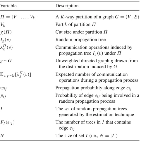
Table 1 Notations used
Variable Description
Π= {V1, . . . ,Vk} AK-way partition of a graphG=(V,E)
Vk Partkof partitionΠ
χ(Π) Cut size under partitionΠ
Ig(v) Random propagation tree
λΠ
g(v) Communication operations induced by
propagation treeIg(v)underΠ
g∼G Unweighted directed graphgdrawn from
the distribution induced byG
Ev,g∼G[λΠg(v)] Expected number of communication
operations during a propagation process
wi j Propagation probability along edgeei j
pi j Probability of edgeei jbeing involved in a
random propagation process
I The set of random propagation trees
generated by the estimation technique
FI(ei j) The number of trees inIthat contains
edgeei j
N The size of setI(i.e.,N = |I|)
Each partVk ∈ Π is a non-empty subset ofV, all parts are mutually exclusive (i.e.,Vk ∩Vm = ∅fork =m), and the union of all parts isV (i.e.,V
k∈ΠVk=V).
Given a partitionΠ, weightWk of a partVkis defined as the sum of the weights of vertices belonging to that part (i.e.,
Wk =v
i∈Vkwi). The partitionΠ is said to be balanced if
all partsVk∈Πsatisfy the following balancing constraint:
Wk ≤Wavg(1+), for 1≤k≤K (1)
Here, Wavg is the average part weight (i.e., Wavg =
vi∈Vwi/K) and is the maximum imbalance ratio of a
partition.
An edge is called cut if its endpoints belong to different parts and uncut otherwise. The cut and uncut edges are also referred to as external and internal edges, respectively. The cut sizeχ(Π)of a partitionΠ is defined as
χ(Π)=
ei j∈EcutΠ
ci j (2)
whereEcutΠ denotes the set of cut edges.
In the multi-constraint extension of the graph partitioning problem, each vertexvi is associated with multiple weights
wc
i forc =1, . . . ,C. For a given partitionΠ,W
c
k denotes
the weight of partVkon constraintc(i.e.,Wkc =vi∈Vkwic). Then,Πis said to be balanced if each partVksatisfiesWkc≤ Wavg(c 1+), whereWavgc denotes the average part weight on constraintc.
minimizes the cut sizeχ(·)in Eq. (2) while satisfying the balancing constraint in Eq. (1) defined on part weights.
2.2 Related work
2.2.1 Graph partitioning and replication
Graph partitioning has been studied to improve scalability and query processing performances of the distributed data management systems. It has been widely used in the context of social networks. Pujol et al. [10] propose a social net-work partitioning solution that reduces the number of edges crossing different parts and provides a balanced distribution of vertices. They aim to reduce the amount of communica-tion operacommunica-tions between servers. It is later extended in [9] by considering replication of some users across different parts. SPAR [11] is developed as a social network partitioning and replication middleware.
Yuan et al. [13] propose a partitioning scheme to process time-dependent social network queries more efficiently. The proposed scheme considers not only the spatial network of social relations but also the time dimension in such a way that users that have communicated in a time window are tried to be grouped together. Additionally, the social graph is partitioned by considering two-hop neighborhoods of users instead of just considering directly connected users. Turk et al. [14] propose a hypergraph model built from logs of temporal user interactions. The proposed hypergraph model correctly encapsulates multi-user queries and is partitioned under load balance and replication constraints. Partitions obtained by this approach effectively reduces the number of communica-tions operacommunica-tions needed during execucommunica-tions of multicast and gather type of queries.
Sedge [3] is a distributed graph management environment based on Pregel [20] and designed to minimize communi-cation among servers during graph query processing. Sedge adopts a two-level partition management system: In the first level, complementary graph partitions are computed via the graph partitioning tool Metis [6]. In the second level, on-demand partitioning and replication strategies are employed. To determine cross-partition hotspots in the second level, the ratio of number of cut edges to uncut edges of each part is computed. This ratio approximates the probability of observ-ing a cross-partition query and later is compared against the ratio of the number of cross-partition queries to internal queries in a workload. This estimation technique differs from our approach, since we estimate an edge being included in a cascade process, whereas this approach estimates the proba-bility of observing a cross-partition query in a part and does not consider propagation processes.
Leopard is a graph partitioning and replication algorithm to manage large-scale dynamic graphs [1]. This algorithm incrementally maintains the quality of an initial
parti-tion via dynamically replicating and reassigning vertices. Nicoara et al. [21] propose Hermes, a lightweight graph repartitioner algorithm for dynamic social network graphs. In this approach, the initial partitioning is obtained via Metis and as the graph structure changes in time, an incremental algorithm is executed to maintain the quality of the partitions. For efficient processing of distributed transactions, Curino et al. [4] propose SCHISM, which is a workload-aware graph model that makes use of past query patterns. In this model, data items are represented by vertices and if two items are accessed by the same transaction, an edge is put between the respective pair of vertices. In order to reduce the number of distributed transactions, the proposed model is split into balanced partitions using a replication strategy in such a way that the number of cut edges is minimized.
Hash-based graph partitioning and selective replication schemes are also employed for managing large-scale dynamic graphs [2]. Instead of utilizing graph partitioning techniques, a replication strategy is used to perform cross-partition graph queries locally on servers. This method makes use of past query workloads in order to decide which vertices should be replicated among servers.
2.2.2 Multi-query optimization
Le et al. [22] propose a multi-query optimization algo-rithm which partitions a set of graph queries into groups where queries in the same group have similar query patterns. Their partitioning algorithm is based on k-means cluster-ing algorithm. Queries assigned to each cluster are rewritten to their cost-efficient versions. Our work diverges from this approach, since we make use of propagation traces to esti-mate a probability distribution over edges in a graph and partition this graph, whereas this approach clusters queries based on their similarities.
2.2.3 Influence propagation
More recently, algorithms that run nearly in optimal linear time and provide(1−1/e)approximation guarantee for the influence maximization problem are proposed in [33–35].
The notion of influence and its propagation processes have also been used to detect communities in social networks. Zhou et al. [36] find community structure of a social network by grouping users that have high influence-based similarity scores. Similarly, Lu et al. [37] and Ghosh et al. [38] consider finding community partition of a social network that maxi-mizes different influence-based metrics within communities. Barbieri et al. [39] propose a network-oblivious algorithm making use of influence propagation traces available in their datasets to detect community structures.
3 Problem definition
In this section, we present the graph partitioning problem within the context of content propagation in a social net-work where the link structure and the propagation probability values associated with these links are given. Let an edge-weighted directed graphG = (V,E, w)represent a social network where each user is represented by a vertexvi ∈ V,
each directed edgeei j ∈ Erepresents the direction of content propagation from uservi tovj and each edgeei j is
associ-ated with a content propagation probabilitywi j ∈ [0,1].
We assume that the wi j probabilities associated with the
edges are known beforehand as in the case of Influence Maximization domain [28,29,34]. Methods for learning the influence/content propagation probabilities between users in a social network are previously studied in the literature [25,26]. In this setting, a partitionΠ ofGrefers to a user-to-server assignment in such a way that a vertexviassigned
to a partVk ∈ Π denotes that the user represented byvi is
stored in the server represented by partVk.
We adopt a widely used propagation model, the IC model, with propagation processes starting from a single user for ease of exposition. As we discuss later, this can be extended to other popular models such as the LT model and propagation processes starting from multiple users as well. Under the IC model, a content propagation process proceeds in discrete time steps as follows: Let a subsetS⊆V consist of initially active users who share a specific content for the first time in a social network (we assume|S| =1 for ease of exposition). For each discrete time stept, let setStconsists of users that are activated in time stept ≥0, which indicates thatS0=S
(i.e., a user becomes activated meaning that this user has just received the content). Once activated in time stept, each uservi ∈ St is given a single chance of activating each of
its inactive neighborvj with a probabilitywi j (i.e., uservi
activates uservj meaning that the content propagates from
vi tovj). If an inactive neighborvj is activated in time step t(i.e.,vjhas received the content), then it becomes active in
the next time stept+1 and added to the setSt+1. The same
process continues until there are no new activations (i.e., until
St = ∅).
Kempe et al. [28] define an equivalent process for the IC model by generating an unweighted directed graph gfrom
Gby independently realizing each edgeei j ∈ Ewith prob-abilitywi j. In the realized graphg, vertices reachable by a
directed path from the vertices in S can be considered as active at the end of an execution of the IC model propagation process starting with the initially active users inS. As a result of the equivalent process of the IC model, the original graph
G induces a distribution over unweighted directed graphs. Therefore, we use the notation g ∼G to indicate that we draw an unweighted directed graphg from the distribution induced byGby using the equivalent process of IC model. That is, we generate a directed graph g via realizing each edgeei j ∈Gwith probabilitywi j.
3.1 Propagation trees
Given a vertex v, we define the propagation tree Ig(v) to denote a directed tree rooted on vertex v in graph g. The tree Ig(v)corresponds to an IC model propagation process, whenv is used as the initially active vertex, in such a way that each edgeei j ∈ Ig(v)encodes the information that the content propagated tovj fromvi during this process. Here,
there can be more than one possible propagation trees forv ong, sinceg may not be a tree itself. One of the possible trees can be computed by performing a breadth-first search (BFS) ongstarting from vertexv, since IC model does not prescribe an order for activating inactive neighbors of the newly activated vertices. Note that generating a graphgand performing a BFS on a vertexvare equivalent to performing a randomized BFS algorithm starting from the vertexv. The difference between the randomized BFS algorithm and usual BFS algorithm is that each edgeei j ∈ E is searched with probabilitywi j in the randomized case. That is, during an
iteration of BFS, if a vertexvi is extracted from the queue,
each of its outgoing edge(s)ei j to an unvisited vertexvj is
examined and added to the queue with a probabilitywi j.
Here, we also define a fundamental concept called ran-dom propagation tree which is used throughout the text. A random propagation tree is a propagation tree that is gener-ated by two levels of randomness: First, a graphgis drawn from the distribution induced by G, then a vertex v ∈ V
u7
S1 S2
S3
u0
u1
u2
u3
u4
u5
u6
u8
u9
0.5|0.27
0.5|0.21
0.9 |0
.32 0.9| 0.34
0.5| 0.05
0.5|0.05
0.5|0
.04 0.5
|0
.05
0.1
|0.
05
0.1
|0.01 0.5
|0
.10 0.5|0.56 0.1|0
.01
0.1|0.01
0.5
|0.
04
(a)
u7
S1 S2
S3
u0
u1
u2
u3
u4
u5
u6
u8
u9 0.5|0.27
0.5| 0.21
0.9 |0
.32 0.9
|0 .34
0.5|0.05
0.5|0.05
0.5|0
.04 0.5|
0.05
0.1
|0.
05
0.1
|0.01 0.5
|0
.10 0.5|0.56 0.1|0
.01
0.1|0.01 0.5|0
.04
(b)
Fig. 1 An IC model propagation instance starting with initially active useru7. Dotted lines denote edges that are not involved in the propagation
process, and straight lines denote edges activated in the propagation process.a,bDisplay the same social network under two different partitions
{S1= {u0,u1,u2},S2= {u6,u7,u8,u9},S3= {u3,u4,u5}}and{S1= {u0,u1,u2,u6},S2= {u7,u8,u9},S3= {u3,u4,u5}}, respectively
all BFS edges. Hence, reverse-reachable sets are different from propagation trees in the ways that they do not consti-tute directed trees and they are built on the structure ofGT
instead ofG.
From a systems perspective, if a content propagation occurs between two users located on different servers, we assume this causes a communication operation. This is depicted in Fig.1which displays a graph with its edges denot-ing directions of content propagations between users. In this figure, two different partitionings of the same social network are given in Fig.1a, b. In Fig.1a, users are partitioned among three servers as S1 = {u0,u1,u2}, S2 = {u6,u7,u8,u9}
andS3 = {u3,u4,u5}. In Fig.1b, user u6 is moved from
S2to S1 where S3remains the same. In the figure, a
con-tent shared by user u7 propagates through four users u6,
u1,u2 andu3under the IC model. Here, the straight lines
denote the edges along which propagation events occurred and these lines constitute the propagation tree formed by this propagation process (probability values associated with the edges will be discussed later in the next section). The dotted lines denote the edges that are not involved in this propaga-tion process. Therefore, in accordance with our assumppropaga-tion, straight lines crossing different parts necessitate communi-cation operations. For instance, in Fig.1a, the propagation of the content fromu7tou6does not incur any communication
operation, whereas the propagation of the same content from
u6tou1andu2incurs two communication operations. For
the whole propagation process initiated by useru7, the total
number of communication operations are equal to 3 and 2 under the partitions in Fig.1a, b , respectively.
Given a partitionΠ ofGand a propagation treeIg(v)of vertexvon a directed graphg∼G, we define the number of
communication operationsλΠg(v)induced by the propaga-tion treeIg(v)under the partitionΠas
λΠg(v)= |{ei j ∈ Ig(v)|ei j ∈EcutΠ}|. (3)
That is, the number of communication operations performed is equal to the number of edges in Ig(v)that are crossing different parts inΠ. It can be observed that each different partitionΠofGinduces a different communication pattern between servers for the same propagation process.
3.2 Cascade-aware graph partitioning
In the cascade-aware graph partitioning problem, we seek to compute a partitionΠ∗ofGthat achieves the following two objectives:
(i) Under the IC model, the expected number of commu-nication operations to be performed between servers during a propagation process starting from a randomly chosen user should be minimized.
(ii) The partition should distribute the users to servers as evenly as possible in order to ensure a balance of work-load among them.
[image:5.595.56.545.51.271.2]equivalence between random propagation trees and random-ized BFS algorithm, the first objective is also equivalent to minimizing the expected number of cross-partition edges tra-versed during a randomized BFS execution starting from a randomly chosen vertex.
To give a formal definition for the proposed problem, we redefine the first objective in terms of the equivalent pro-cess of the IC model. For a given partitionΠ of G, we write the expected number of communication operations to be performed during a propagation process starting from a randomly chosen user asEv,g∼G[λΠg(v)]. Here, subscripts
v andg ∼ G of the expectation function denote the two levels of randomness in the process of generating a random propagation tree. As mentioned above, a random propagation tree Ig(v)is equivalent to a propagation process that starts from a randomly chosen user in the network. Therefore, the expected value ofλΠg(v), which denotes the expected number
of cut edges included in a random propagation tree, is equiv-alent to the expected number of communication operations to be performed. Due to this correspondence, computing a partitionΠ∗that minimizes the expectationEv,g∼G[λΠg(v)]
achieves the first objective (i) of the proposed problem. Con-sequently, the proposed problem can be defined as a special type of graph partitioning in which the objective is to compute a K-way partitionΠ∗ ofG that minimizes the expectation
Ev,g∼G[λΠg(v)]subject to the balancing constraint in Eq. (1).
That is,
Π∗=argmin
Π Ev,g∼G[λ
Π
g(v)] (4)
subject toWk ≤Wavg(1+)for allVk ∈Π. Here, we des-ignate weightwi =1 of each vertexvi ∈V and define the
weightWk of a partitionVk ∈Π as the number of vertices assigned to that part (i.e.,Wk = |Vk|). Therefore, this bal-ancing constraint ensures that the objective (ii) is achieved by the partitionΠ∗.
4 Solution
The proposed approach is to first estimate a probability distri-bution for modeling the propagation and use it as an input to map the problem into a graph partitioning problem. Given an edge-weighted directed graph G = (V,E, w) repre-senting an underlying social network, the first stage of the proposed solution consists of estimating a probability dis-tribution defined over all edges ofG. For that purpose, we define a probability value pi j for each edgeei j ∈ E apart from its content propagation probabilitywi j. The value pi j
of an edgeei j is defined to be the probability that the edge
ei j is involved in a propagation process that starts from a randomly selected user. Equivalently, when a random
prop-agation tree Ig(v)is generated by the process described in Sect. 3, the probability that the edgeei j is included in the propagation treeIg(v)is equal to pi j. It is important to note that the valuewi j of an edgeei jcorresponds to the
probabil-ity that the edgeei jis included in a graphg∼G, whereas the value pi j is defined to be the probability thatei j is included in a random propagation tree Ig(v) rooted on a randomly selected vertexvin graphg. For now, we delay the discus-sion on the computation of pi j values for ease of exposition and assume that we are provided with the pi j values. Later in this section, we provide an efficient method that estimates these values.
The functionEv,g∼G[λΠg(v)]corresponds to the expected
number of cut edges in a random propagation tree Ig(v)
under a partition Π. In other words, if we draw a graphg
from the distribution induced byGand randomly choose a vertex v and compute its propagation tree Ig(v), then the expected number of cut edges included in Ig(v)is equal to
Ev,g∼G[λΠg(v)]. On the other hand, the valuepi jof an edge ei jis defined to be the probability that the edgeei jis included in a random propagation tree Ig(v). Therefore, given a par-titionΠofG, the functionEv,g∼G[λΠg(v)]can be written in
terms of pi j values of all cut edges inEcutΠ as follows:
Ev,g∼G[λΠg(v)] =
ei j∈EcutΠ
pi j (5)
In Eq. (5), the expected number of cut edges in a random propagation tree is computed by summing the pi j value of each edgeei j ∈ EcutΠ, where the value pi j of an edgeei j is
defined to be the probability that the edgeei jis included in a random propagation tree. Hence, the main objective becomes to compute a partitionΠ∗that minimizes the total pi j val-ues of edges crossing different parts inΠ∗and satisfies the balancing constraint defined over the part weights. That is,
Π∗=argmin
Π
ei j∈EcutΠ
pi j (6)
subject to the balancing constraint defined in the original problem. As mentioned earlier, each vertexvi is associated
with a weightwi = 1 and part weight Wi of a partVi is
defined to be the number of vertices assigned to Vi (i.e.,
Wi = |Vi|).
LetΠ be a partition ofG. SinceGandGconsist of the same vertex setV,Π induces a setEcutΠ of cut edges for the original graphG. Due to the cost definitions of edges inE, the cut sizeχ(Π)ofGunder partitionΠis equal to the sum of the pi j values of cut edges inEcutΠ which is shown to be equal to the value of the main objective function in Eq. (4). That is,
χ(Π)=
ei j∈EcutΠ
pi j =Ev,g∼G[λΠg(v)] (7)
Hence, a partitionΠ∗that minimizes the cut sizeχ(·)ofG
also minimizes the expectationEv,g∼G[λΠg(v)]in the
origi-nal social network partitioning problem. In other words, if the partitionΠ∗forGis an optimal solution for the partitioning ofG, it is also an optimal solution for Eq. (4) in the orig-inal problem. Additionally, the equivalence drawn between the graph partitioning problem and the cascade-aware graph partitioning problem also proves that the proposed problem is NP-Hard even thepi j values were given beforehand.
In Fig.1, the main objective of cascade-aware graph par-titioning is depicted as follows: Each edge in the figure is associated with a content propagation probability along with its computedpi j value (i.e., each edgeei j is associated with “wi j | pi j”). The partitioning in Fig. 1a provides a better
cut size in terms of both number of cut edges and the total propagation probabilities of edges crossing different parts. However, we assert that the partitioning in Fig.1b provides a better partition for objective function4, at the expense of pro-viding worse cut size in terms of other cut size metrics (i.e., the sum ofpi j values of cut edges is less in the second par-tition).
4.1 Computation of the
p
ijvalues
We now return to the discussion on the computation of thepi j
values defined over all edges ofGand start with the following theorem indicating the hardness of this computation:
Theorem 1 Computation of the pi j value for an edge ei j of G is a#P-Hard problem.
Proof Let functionσ(vk, vi)denote the probability of there
being a directed path from vertexvkto vertexvion a directed
graphgdrawn from the distribution induced byG. Assume that the only path goes fromvk tovj is throughvi on each
possibleg. That is vj is only connected tovi inG. (This
simplifying assumption does not affect the conclusion we draw for the theorem.) Hence, the probability ofviincluded
in a propagation treeIg(vk)isσ(vk, vi). Let pi jk denote the
probability ofei j is included inIg(vk). We can compute pki j
as
pki j =wi j·σ (vk, vi) (8)
since inclusion ofei j ing and formation of a directed path from vk tovi ong are two independent events; therefore,
their respective probability valueswi j andσ(vk, vi)can be
multiplied. As mentioned earlier, the value pi j of an edge
ei j is defined to be the probability of edgeei j included in a random propagation tree. Therefore, we can compute the value pi j of an edgeei j as follows:
pi j = 1 |V|
vk∈V
pi jk (9)
Here, to compute the pi j value of edge ei j, we sum the conditional probability |V1|·pki j for allvk ∈ V. Due to the
definition of random propagation trees, selections of vk in
a graphg ∼Gare all mutually exclusive events with equal probability|V1|. Therefore, we can sum the terms|V1| ·pi jk for eachvk∈V to compute the total probability pi j.
In order to prove the theorem, we present an equivalence between the computation of function σ(·,·) and the s,t -connectedness problem [41], since thepi jvalue of an edgeei j
depends on the computation ofσ(vk, vi)for allvk ∈V. The
input to thes,t-connectedness problem is a directed graph
G =(V,E), where each edgeei j ∈ E may fail randomly and independently from each other. The problem asks to com-pute the total probability of there being an operational path from a specified source vertexs to a target vertext on the input graph. However, computing this probability value is proven to be a #P-Hard problem [41]. On the other hand, the functionσ(vk, vi)denotes the probability of there being a
directed path fromvktovi in ag∼G, where each edge ing
is realized with probabilitywi jrandomly and independently
from other edges. It is obvious to see that the computation of functionσ(vk, vi)is equivalent to the computation of the s,t-connectedness probability. (We refer the reader to [17] for a more formal description for the reduction ofσ(vk, vi)
tos,t-connectedness problem). This equivalence implies that the computation of functionσ(vk, vi)is #P-Hard even for a
single vertexvk and therefore implies that the computation
of pi jvalue for any edgeei j is also #P-Hard.
Theorem 1states that it is unlikely to devise a polyno-mial time algorithm which exactly computes pi j values for all edges in G. Therefore, we employ an efficient method that can estimate thesepi jvalues for all edges inGat once. These estimations can be made within a desired level of accu-racy and confidence interval, but there is a trade-off between the runtime and the estimation accuracy of the proposed approach. On the other hand, the quality of the results pro-duced by the overall solution is expected to increase with increasing accuracy of the pi j values.
is generated by first drawing a directed graphg ∼G and then computing a propagation treeIg(v)ongfor a randomly selected vertexv∈V. LetI be the set of all random propa-gation trees generated for estimation and letNbe the size of this set (i.e.,N = |I|). After forming the setI, the valuepi j
of an edgeei jcan be estimated by the frequency of that edge’s appearance in random propagation trees inI as follows: Let functionFI(ei j)denote the number of random propagation trees inI that contains edgeei j. That is,
FI(ei j)= |{Ig(v)∈I |ei j ∈Ig(v)}| (10)
Due to the definition ofpi j, the appearance of edgeei j in a random propagation tree Ig(v) ∈ I can be considered as a Bernoulli trial with success probability pi j. Hence, the function FI(ei j)can be considered as the number of total successes inNBernoulli trials with success probability pi j, which implies that FI(ei j) is Binomially distributed with parameters N and pi j (i.e., FI(ei j)∼Binomial(pi j,N)). Therefore, the expected value of the functionFI(ei j)is equal topi jN, which also implies that
pi j =E[FI(ei j)/N] (11)
As a result of Eq. (11), if an adequate number of random propagation trees are generated to form the setI, the value
FI(ei j)/Ncan be an estimation for the value of pi j. There-fore, the estimation method consists of generatingNrandom propagation trees that together form the setI, and comput-ing the functionFI(ei j)according to Eq. (10) for each edge
ei j ∈ E. After computing the functionFI(ei j)for each edge
ei j, we useFI(ei j)/N as an estimation for the pi j value.
4.2 Implementation of the estimation method
We seek an efficient implementation for the proposed estima-tion method. The main computaestima-tion of the method consists of generatingNrandom propagation trees. A random prop-agation tree can be efficiently generated by performing a randomized BFS, starting from a randomly chosen vertex, inG. It is important to note that the randomized BFS algo-rithm starting from a vertexvis equivalent to drawing a graph
g ∼Gand performing a BFS starting from the vertexvon
g. That is, the randomized BFS algorithm is equivalent to the method introduced in Sect.3to generate a propagation treeIg(v)rooted onv. Therefore, forming the set I can be accomplished by performingNrandomized BFS algorithms onGstarting from randomly chosen vertices. Moreover, the computation of the functionFI(·)for all edges inE can be performed while forming the setIwith a slight modification to the randomized BFS algorithm. For this purpose, a counter for eachei j ∈ E can be kept in such a way that its value is incremented each time the corresponding edge is traversed
during a randomized BFS execution. This counter denotes the number of times an edge is traversed during the perfor-mance of all randomized BFS algorithms. Therefore, after
N randomized BFS executions, the functionFI(ei j)for an edgeei j is equal to the value of the counter maintained for that edge.
4.3 Algorithm
The overall cascade-aware graph partitioning algorithm is described in Algorithm1. In the first line, the setIis formed by performing N randomized BFS algorithms, where the function FI(ei j)is computed for each edge ei j ∈ E dur-ing these randomized BFS executions. In lines 2 and 3, an undirected graph G = (V,E)is built via composing a new setEof undirected edges, where each undirected edge
ei j ∈ Eis associated with a cost ofci jusing the estimations computed in the first step. In line 4, each vertexvi ∈ V is
associated with a weightwi =1 in order to ensure that the
weight of a part is equal to the number of vertices assigned to that part. Lastly, a K-way partitionΠof the undirected graph
Gis obtained using an existing graph partitioning algorithm and returned as a solution for the original problem. Here, the graph partitioning algorithm is executed with the same imbalance ratio as with the original problem.
4.4 Determining the size of set
I
As mentioned earlier, the accurate estimation of thepi j val-ues is a crucial step to compute “good” solutions for the proposed problem, since the graph partitioning algorithm used in the second step makes use of these pi j values to compute the costs of edges inG. The total cost of cut edges
Algorithm 1Cascade-Aware Graph Partitioning
Input:G=(V,E, w),K,
Output:Π
1: Form a setIofNrandom propagation trees by performing
random-ized BFS algorithms onGand computeFI(ei j)for eachei j ∈E
according to Eq. (10)
2: Build an undirected graphG=(V,E)where edge setEis
com-posed as follows:
E= {ei j |ei j∈E∨ej i ∈E} (12)
3: Associate a costci jwith eachei j ∈Eas follows:
ci j= ⎧ ⎪ ⎨ ⎪ ⎩
FI(ei j)/N+FI(ej i)/N, if ei j∈E∧ej i ∈E
FI(ei j)/N, if ei j∈E∧ej i ∈/E
FI(ej i)/N, if ei j∈/E∧ej i ∈E
(13)
4: Associate each vertexvi∈Vwith weightwi=1.
5: Compute aK-Way partitionΠofGusing an existing graph
parti-tioning algorithm (using the same imbalance ration).
inGrepresents the value of the objective function in Eq. (4). Therefore, thepi j values need to be accurately estimated so that the graph partitioning algorithm correctly optimizes the objective function.
Estimation accuracies of the pi j values depend on the number of random propagation trees forming the setI. As the size of the setIincreases, more accurate estimations can be obtained. However, we want to compute the minimum value ofN to get a specific accuracy within a specific confidence interval. More formally, let pi jˆ be the estimation computed for thepi j value of an edgeei j ∈ E(i.e.,pi jˆ =FI(ei j)/N), and we want to compute the minimum value ofNto achieve the following inequality:
Pr[| ˆpi j−pi j| ≤θ ,∀ei j ∈E] ≥1−δ. (14)
That is, with a probability of at least 1−δ, we want the estimation pi jˆ to be within θ of pi j for each edge ei j ∈ E. For that purpose, we make use of well-known Chernoff [42] and Union bounds from probability theory. Chernoff bound can be used to find an upper bound for the probability that a sum of many independent random variables deviates a certain amount from their expected mean. In this regard, due to the function FI(·)being Binomial, Chernoff bound can guarantee the following inequality:
Pr |FI(ei j)−pi jN| ≥ξpi jN≤2 exp
− ξ2
2+ξ ·pi jN
(15)
for each edgeei j ∈ E. Here,ξdenotes the distance from the expected mean in the context of Chernoff bound.
In Eq. (15), dividing both sides of the inequality|FI(ei j)− pi jN| ≥ξ pi jNin the functionPr[·]byN and takingξ =
θ/pi jyields
Pr[| ˆpi j−pi j| ≥θ] ≤2 exp
− θ2 2pi j +θ ·N
≤2 exp
− θ2 2+θ ·N
(16)
which denotes the upper bound for the probability that the accuracyθ is not achieved for a single edgeei j (the last inequality in Eq. (16) follows, since pi j ≤ 1). Moreover, RHS of Eq. (16) is independent from the value of pi j and its value is the same for all edges inE, which enables us to apply the same bound for all of them. However, our objective is to find the minimum value ofNto achieve accuracyθfor all edges simultaneously with a probability at least 1−δ. For that purpose, we need to find an upper bound for the probability that there exists at least one edge inEfor which the accuracyθis not achieved. We can compute this upper
bound using Union bound as follows:
Pr[| ˆpi j −pi j| ≥θ ,∃ei j ∈ E] ≤2|E|exp
− θ2 2+θ ·N
(17)
Here, we simply multiply RHS of Eq. (16) by|E|, since for each edge inE, the accuracyθis not achieved with a proba-bility at most 2 exp(−2θ+2θ ·N). In order to achieve Eq. (14), RHS of Eq. (17) needs to be at mostδ. That is,
2|E|exp
− θ2 2+θ ·N
≤δ (18)
Solving this equation forN yields
N ≥ 2+θ
θ2 ·ln
2|E|
δ (19)
which indicates the minimum value ofNto achieveθ accu-racy for all edges inE with a probability at least 1−δ.
The accuracyθdetermines how much error is made by the graph partitioning algorithm while it performs the optimiza-tion. As shown in Eq. (7), for a partitionΠofGobtained by the graph partitioning algorithm, the cut sizeχ(Π)is equal to the value of main objective function (4). However, the cost values associated with the edges ofGare estimations of their exact values, and therefore, the partition costχ(Π)might be different from the exact value of the objective function. In this regard, the difference between the objective function and the partition cost can be expressed as follows:
Ev,g∼G[λΠg(v)] −χ(Π)≤θ· |EcutΠ| (20)
Here, the error is computed by multiplying the accuracyθ by the number of cut edges ofGunder the partitionΠ, since for each edge inEcutΠ, at mostθ error can be made with a probability at least 1−δ. Therefore, even if it were possible to solve the graph partitioning problem optimally, the solution returned by Algorithm 1 would be withinθ · |EcutΠ| of the optimal solution for the original problem with a probability at least 1−δ. Consequently, as the value of θ decreases, the partition obtained by Algorithm 1will incur less error for the main objective function, which will enable the graph partitioning algorithm to perform a better optimization for the original problem.
4.5 Complexity analysis
The proposed algorithm consists of two main computa-tional phases. In the first phase, for an accuracy θ with confidenceδ, the setI is generated via performing at least
N = 2θ+2θ ·ln
2|E|
these BFS executions takes Θ(V + E) time. The second phase of the algorithm performs the partitioning of the undi-rected graph G which is constructed from the directed graph G by using FI(ei j) values computed in the first phase. The construction of the graphG can be performed inΘ(V+E)time. The partitioning complexity of the graph
G, however, depends on the partitioning tool used. In our implementation, we preferred Metis which has a complexity ofΘ(V+E+KlogK), whereKis the number of partitions. Therefore, ifθandδare assumed to be constants, the overall complexity of Algorithm1to obtain aK-way partition can be formulated as follows:
Θ
2+θ
θ2 ln
2|E|
δ (V+E)
+Θ(V+E+KlogK) =Θ((V+E)logE+KlogK). (21)
Equation (21) denotes serial execution complexity of Algorithm 1. The proposed algorithm’s scalability can be improved even further via parallel processing, since the esti-mation technique is embarrassingly parallel. GivenPparallel processors,Npropagation trees inIcan be computed without necessitating any communication or synchronization (i.e., each processor can generateN/Ptrees by separate BFS exe-cutions). The only synchronization point is needed in the reduction of FI(ei j)values computed by these processors. This reduction operation, however, can be efficiently per-formed in logPsynchronization phases. Additionally, there exist parallel graph partitioning tools (e.g., ParMetis [43]) which can improve the scalability of the graph partitioning phase.
4.6 Extension to the LT model
Even though we have illustrated the problem and solution for the IC model, both our problem definition and proposed solution can be easily extended to other models such as the LT (linear threshold) model. It is worth to mention that the proposed solution does not depend on the IC model or the probability distribution defined over edges (i.e.,wi j
prob-abilities). As long as the random propagation trees can be generated, the proposed solution does not require any mod-ification for the use of any different cascade model or the probability distribution defined over edges.
We skip the description for the LT model and just provide the equivalent process of LT model proposed in [28]. In the equivalent process of the LT model, an unweighted directed graphgis generated fromGby realizing only one incoming edge of each vertex inV. That is, for each vertexvi ∈ V,
each incoming edgeej i of vertexvi has probabilitywj i of
being selected and only the selected edge is realized ing. Given a directed graphg generated by this equivalent pro-cess, a propagation tree Ig(v)rooted on vertexvagain can
be computed by performing a BFS starting fromvong. Dif-ferent from the equivalent process of IC model, there can be only one propagation tree for each vertex, since all vertices have only one incoming edge to these vertices. However, a propagation treeIg(v)under LT model still encodes the same information as in IC model; that is, each edgeei j ∈ Ig(v)
encodes the information that a content propagates fromvi to
vj.
In the problem definition part, we make use of the notion of propagation trees in such a way that edges in a propa-gation tree that are crossing different parts are assumed to necessitate communication operations between servers. This assumption also holds for the LT model, since propagation trees generated by the equivalent processes of IC and LT mod-els encode the same information. Therefore, minimizing the expected number of communication operations during an LT propagation process starting from a randomly chosen user still corresponds to minimizing the expected number of cut edges in a random propagation tree. In this regard, we do not need any modification for the objective function (4) and we still want to compute a partitionΠ∗ that minimizes the expected number of cut edges in a random propagation tree. (The only difference is in the process of computing a random propagation tree under LT model.)
In the solution part, we generate a certain number of random propagation trees in order to estimate a probabil-ity distribution defined over all edges in E. The estimated probability distribution associates each edge with a proba-bility value denoting how likely an edge is included in a random propagation tree under the IC model. The associated probability values are also later used as costs in the graph par-titioning phase. However, both the estimation method and the overall solution do not depend on anything specific to the IC model and only require a method for generating ran-dom propagation trees which is mentioned above. Moreover, concentration bounds attained for the estimation of the prob-ability distribution still holds under the LT model and the number of random propagation trees forming the set I in Algorithm1should satisfy Eq. (19).
4.7 Processes starting from multiple users
vertex can be arbitrarily included in one of the propagation trees rooted on these vertices. As noted earlier, the IC model does not prescribe an order for activating inactive neighbors; therefore, a random propagation forest over the setScan be computed by first drawing a graphg∼Gand then perform-ing a multi-source BFS ongstarting from the vertices inS. The order of execution of multi-source BFS determines the form of propagation trees in the propagation forestIg(S).
In a partitionΠof propagation forestIg(S), each cut edge incurs one communication operation. So, the total number of communication operations induced byΠis defined to be the number of cut edges which we denote asλΠg(S). These new definitions do not require any major modification for the opti-mization problem introduced in Eq. (4), and we just replace the expectation function withEv,g∼G[λΠg(S)]. That is, our
objective becomes computing a partition that minimizes the expected number of cut edges in a random propagation forest.
To generalize the proposed solution, we redefinepi jvalue of an edgeei j as the probability of edgeei j included in a random propagation forest instead of a random propagation tree. With this new definition ofpi j values, Eqs. (5) and (6) can still be satisfied; hence, a partitionΠ∗ that minimizes the sum of pi j values of edges crossing different parts also minimizes the expectationEv,g∼G[λΠg(S)].
The new definition ofpi j values necessitates some modi-fications to the estimation method proposed earlier. Recall that, for the previous definition of pi j values, we gener-ate a set I of random propagation trees and compute the functionFI(·)for each edgeei j. For the new definition of
pi j values, the estimations can be obtained with a similar approach; however, the set I must now consist of random propagation forests and FI(·)must denote frequencies of edges to appear in these random propagation forests. There-fore, the only modification required for Algorithm1 is to replace the step that the setI is generated by performingN
randomized BFS algorithms. The new setI of random prop-agation forests can be obtained with a similar approach such that instead of performing randomized single-source BFS algorithms, we perform randomized multi-source BFS algo-rithms. These two BFS algorithms are essentially the same except that multi-source BFS starts execution with its queue containing a randomly selected subset of vertices instead of a single vertex. The new definitions together with the modi-fications performed on the overall solution do not affect the concentration bounds obtained in Eq. (19).
5 Extensions and limitations
Here, we show how the proposed cascade-aware graph parti-tioning algorithm (CAP) can be incorporated into other graph partitioning objectives.
5.1 Non-cascading queries
Queries such as “reading-friend’s-posts” and “read-all-posts-from-friends” can be observed more frequently than cascad-ing (i.e., re-share) operations in a typical OSN application. The number of communication operations for such non-cascading queries may require minimizing the number of cut edges if query workload is highly changing or not avail-able, or minimizing the total traffic crossing different parts if it can be estimated. The cascade-aware graph partition-ing aims at reducpartition-ing the cut edges that have high probability of being involved in a random propagation process under a specific cascade model. Assigning unit weights to all edges (i.e.,ci j = 1 for each edgeei j) makes the objective same as minimizing the number of cut edges. A combination of objectives can be achieved by assigning each edge cost
ci j = 1+α(pi j + pj i), whereα determines the relative
weight of traffic/cascade-awareness.
5.2 Intra-propagation balancing among servers
This paper considers the number of nodes/users as the only balancing criteria for the proposed cascade-aware partition-ing. On the other hand, the proposed formulation can be enhanced to handle balance on multiple workload metrics via a multi-constraint graph partitioning. For example, a balanced distribution of the number of content propagation operations within servers can be attained via the follow-ing two-constraint formulation. We assign the followfollow-ing two weights to each vertexvi:
w1
i =1 and w2i =
eki∈E
pki. (22)
Here, the summation in the second weight represents the sum of pprobabilities of the incoming edges of vertexvi. Under
this vertex weight definition, the two-constraint partitioning maintains balance on both the number of users assigned to servers and the number of intra-propagation operations to be performed within servers. The latter balancing holds because of the fact that the expected number of propagations within a partVkis
ei j∈E(Vk)
pi j (23)
where E(Vk)denotes the set of edges pointing toward the vertices inVk.
5.3 Repartitioning
nec-essary [1–3,21]. Repartitioning methods aims to maintain the quality of an initial partition via reassigning vertices to parts as the graph structure changes. However, the costs of new edges should be computed for repartitioning. That is, if a new direct edge is established inG, then its p value needs to be computed before repartitioning. Thepi jvalue of a new edgeei j can be computed usingpkivalue of each incoming edgeeki of vertexvias follows:
pi j =wi j× ⎡ ⎣1−
eki∈E
(1−pki)
⎤
⎦ (24)
That is, the content propagation probabilitywi jis multiplied
by the probability of there being at least one edgeeki incom-ing to vertexvi is activated during a random propagation
process. It is important to note that establishing the new edge
ei jalso affectspj kvalue of each outgoing edgeej kof vertex
vj. If these values also need to be updated during
repartition-ing, Eq.(24) can be applied for each edgeej k, in succession
for updating the value ofpi j. In short, while moving vertices between parts during repartitioning, thepi jvalue of any edge
ei j can be updated via applying Eq. (24) in a correct order. By updatingpi j values on demand, the existing repartition-ing approaches can be adapted for the cascade-aware graph partitioning problem.
5.4 Replication
Replication strategies need some modifications in order to be used for the cascade-aware graph partitioning. It should be noted that, even though the cut size of graph
G can be reduced via replication of some vertices among multiple parts, this approach also incurs additional commu-nication operations. This is because, when a replicated vertex becomes active during a content propagation process, the content needs to be transferred to each server that the vertex is replicated.
6 Experimental evaluation
In this section, we experimentally evaluate the perfor-mance of the proposed solution on social network datasets. We develop an alternative solution, which produces compet-itive results, as a baseline algorithm in our experiments. The baseline algorithm directly makes use of propagation prob-abilities between users in the partitioning phase (i.e., wi j
values). Additionally, we also test various algorithms previ-ously studied in the literature [10,13] and compared them with the proposed solution.
6.1 Experimental setup
6.1.1 Datasets
Table2displays the properties of the real-world social net-works used in our experiments. Many of these datasets are used in the context of influence maximization research [34]. The first 13 datasets (Facebook–LiveJournal) are collected from Stanford Large Network Dataset Col-lection1 [45], and they contain friendship, communication or citation relationships between users in various real-world social network applications. Twitter (large) is collected from [46], uk-2002 and webbase-2001 are collected from Laboratory for Web Algorithmics2[47],
and sinaweibo is collected from Network Repository3 [48]. Additionally, we also make use of a synthetic graph, named as random-social-network, which we gen-erate by using graph500 [49] power law random graph generator. The graph500 tool is initialized with two param-eters, namely asedge-factorandscale, in order to produce graphs with 2scalevertices and edge-factor×2scale directed edges. We set bothscaleandedge-factor to 16 to produce random-social-networkdataset.
All datasets are provided in the form of a graph, where users are represented by vertices and relationships by directed or undirected edges. To infer the direction of content propa-gation between users, we interpret these social networks as follows: For directed graphs, we assume that a propagation may occur only in the direction of a directed edge, whereas for undirected graphs, we assume that a propagation may occur in both directions along an undirected edge. Therefore, we did not apply any modifications to the directed graphs, whereas we modified the undirected graphs by replacing each undirected edge with two opposite directed edges.
In the datasets in Table2, the information about the con-tent propagation probabilities between users is not available. Therefore, for each dataset, we draw values uniformly at random from the interval [0,1] and associate these values with the edges connecting its pairs of users as the propa-gation probabilities. We repeat this process five times for each dataset and obtain five different versions of the same social network having different propagation probabilities associated with its edges. Using these versions of the social network, we performed the same set of experiments on each different version and reported the averages of the results obtained for that specific dataset.
Given an underlying social network with its associated propagation probabilities, our aim is to find a user partition that minimizes the expected number of communication
oper-1 https://snap.stanford.edu/data.
2 http://law.di.unimi.it.
ations during a random propagation process under a specific cascade model. There have been effective approaches in the literature to learn the propagation probabilities between users in a social network [25,26]. Inferring these probability values using logs of user interactions is out of the scope of this paper. However, we also work on a real-world dataset, from which real propagation traces can be deduced, to test the proposed solution.
6.1.2 Baseline partitioning (BLP) algorithm
One can partition the input graph in such a way that the edges with high propagation probabilities are removed from the cut as much as possible. To achieve this, the sum of prop-agation probabilities of the cut edges can be considered as an objective function to be minimized in the graph partitioning problem. The baseline algorithm also builds an undirected graph from a given social network and makes use of a graph partitioning tool. Instead of computing a new probability dis-tribution over all edges (i.e., the pi j values), the baseline algorithm directly makes use of propagation probabilities associated with edges (i.e., thewi j values). That is, the cost ci j of an undirected edgeei j ofGis determined usingwi j
andwj i values instead of pi j and pj i values of edgesei j
andej i, respectively. By this way, the graph partitioner min-imizes the sum of propagation probabilities associated with the edges crossing different parts. The difference between the baseline algorithm and the proposed solution is the cost values associated with the edges of the undirected graph pro-vided to the graph partitioner.
6.1.3 Other tested algorithms
In our experiments, we also test three previously studied social network partitioning algorithms for comparison pur-poses. The first of these algorithms (CUT) is given in [10] and aims to minimize the number of links crossing differ-ent parts (i.e., basically minimizes the number of cut edges). The second algorithm (MO+) [10] makes use of a commu-nity detection algorithm and performs partitioning based on the community structures inherent to social networks.
As the third algorithm, we consider the social network partitioning algorithm provided in [13]. The social graph is partitioned in such a way that two-hop neighborhood of a user is kept in one partition, instead of the one-hop network. For that purpose, an activity prediction graph (APG) is built and its edges are associated with weights that are computed using the number of messages exchanged between users in a time period. Since thewi j values can not be directly considered
as the number of messages exchanged between users, we make use of FI(ei j)values computed by CAP algorithm. That is, we designate the number of messages exchanged in a time period between users asFI(ei j). Additionally, to
compute edge weights, the algorithm uses two parameters which are the total number of past periods considered and a scaling constant (these parameters are referred to asK and
Cin [13]). We set these parameters toone, since we can not partitionFI(ei j)values into time periods. Using these values, we construct the same APG graph and partition this graph. We refer to this algorithm as 2Hop in our experiments.
6.1.4 Content propagations
To evaluate the qualities of the partitions obtained by the tested algorithms, we performed a large number of experi-ments based on both real and IC-based traces of propagation on real-world social networks. We generated the IC-based propagation data as follows: First, we generate a randomly selected subset of users and then execute an IC model prop-agation process starting from the users in this set. The size of the set is randomly determined and chosen uniformly at random from the interval [1,50]. During this propagation process, we count the total number of propagation events that occurred between the users located on different parts. As mentioned earlier, such propagation events cause communi-cation operations between servers according to our problem definition. For each of the datasets, we perform 105 such experiments and compute the average of the total number of communication operations performed under a given par-tition. This average corresponds to an estimation for the expected number of communication operations during a ran-dom propagation process.
6.1.5 Partitioning framework
The graphs generated by algorithms, except MO+, are par-titioned using state-of-the-art multi-level graph partitioning tool Metis [6] using the following set of parameters: We spec-ify partitioning method as multi-level k-way partitioning, type of objective as edge-cut minimization and the maximum allowed imbalance ratio as 0.10. All the other parameters are set to their default values. We implemented MO+ algorithm by using a community detection algorithm4provided in [50] with its default parameters.
In order to observe the variation of the relative perfor-mance of the algorithms, each graph instance is partitioned
K-way for K = 32,64,128,256,512 and 1024, respec-tively. In order to observe the performance gain achieved by intelligent partitioning algorithms, all graph instances are also partitioned random-wise, which is referred to as random partitioning (RP) algorithm.


![Fig. 2 The geometric means of the communication operation countsand 2Hop [incurred by the partitions obtained by BLP, CUT [10], CAP, MO+ [10]13] normalized with respect to those by RP](https://thumb-us.123doks.com/thumbv2/123dok_us/9428688.447842/15.595.53.287.52.197/geometric-communication-operation-countsand-incurred-partitions-obtained-normalized.webp)


