warwick.ac.uk/lib-publications
Original citation:
Li, Bin, Guo, Weisi, Liang, Y., An, C. and Zhao, Chenglin (2018) Asynchronous device detection
for cognitive device-to-device communications. IEEE Transactions on Wireless
Communications. doi:
10.1109/TWC.2018.2796553
Permanent WRAP URL:
http://wrap.warwick.ac.uk/97425
Copyright and reuse:
The Warwick Research Archive Portal (WRAP) makes this work by researchers of the
University of Warwick available open access under the following conditions. Copyright ©
and all moral rights to the version of the paper presented here belong to the individual
author(s) and/or other copyright owners. To the extent reasonable and practicable the
material made available in WRAP has been checked for eligibility before being made
available.
Copies of full items can be used for personal research or study, educational, or not-for profit
purposes without prior permission or charge. Provided that the authors, title and full
bibliographic details are credited, a hyperlink and/or URL is given for the original metadata
page and the content is not changed in any way.
Publisher’s statement:
“© 2018 IEEE. Personal use of this material is permitted. Permission from IEEE must be
obtained for all other uses, in any current or future media, including reprinting
/republishing this material for advertising or promotional purposes, creating new collective
works, for resale or redistribution to servers or lists, or reuse of any copyrighted component
of this work in other works.”
A note on versions:
The version presented here may differ from the published version or, version of record, if
you wish to cite this item you are advised to consult the publisher’s version. Please see the
‘permanent WRAP URL’ above for details on accessing the published version and note that
access may require a subscription.
Asynchronous Device Detection for Cognitive
Device-to-Device Communications
Bin Li,
Member, IEEE
, Weisi Guo,
Senior Member, IEEE
, Ying-Chang Liang,
Fellow, IEEE
, Chunyan An,
Chenglin Zhao
Abstract—Dynamic spectrum sharing will facilitate the in-terference coordination in device-to-device (D2D) communica-tions. In the absence of network level coordination, the timing synchronization among D2D users will be unavailable, leading to inaccurate channel state estimation and device detection, especially in time-varying fading environments. In this study,
we design anasynchronousdevice detection/discovery framework
for cognitive-D2D applications, which acquires timing drifts and dynamical fading channels when directly detecting the existence of a proximity D2D device (e.g. or primary user). To model and analyze this, a new dynamical system model is established, where the unknown timing deviation follows a random process, while the fading channel is governed by a discrete state Markov chain. To cope with the mixed estimation and detection (MED) problem, a novel sequential estimation scheme is proposed, using the conceptions of statistic Bayesian inference and random finite set. By tracking the unknown states (i.e. varying time deviations and fading gains) and suppressing the link uncertainty, the proposed scheme can effectively enhance the detection performance. The general framework, as a complimentary to a network-aided case with the coordinated signaling, provides the foundation for development of flexible D2D communications along with proximity-based spectrum sharing.
Index Terms—D2D, spectrum sharing, out-of-coverage, device discovery/detection, asynchronous detection, Bayesian inference
I. INTRODUCTION
D
EVICE to device (D2D) communications, which exploit the natural proximity of randomly distributed devices and establish a direct link between two neighbors without routing via based-station (BS) [1], [2], constitute an appealing way to flexibly deploy future wireless networks. By offering the prospect of improved resource utilization (i.e. both the spectrum and energy efficiency), D2D may also effectively alleviate the bottleneck effect of BS and thereby promotes the overall throughput of cellular networks [3], [4]. In this regards, D2D has the potential to accommodate for the expected ex-plosion in the number of wireless devices (e.g. 10×increasing in 2019) [5], and forms part of the envisaged 5G ultra-dense networks [6], [7].Bin Li and Chenglin Zhao are with the School of Information and Com-munication Engineering (SICE), Beijing University of Posts and Telecommu-nications (BUPT), Beijing, 100876, China. (Email: [email protected]).
Weisi Guo is with School of Engineering, University of Warwick, West Midlands, CV47AL. (Email: [email protected])
Y.-C. Liang is with School of Electrical and Information Engineering, University of Sydney, NSW 2006, Australia, and also with University of Electronic Science and Technology of China (UESTC), Chengdu 611731, China. (e-mail: [email protected])
Chunyan An is with State Grid Corporation of China (SGCC), Global Energy Internet Research Institute (GEIRI), Beijing, 102209, China. (Email: [email protected])
In D2D, despite the benefits of centralized coordination from BS [8]–[10], minimal involvement of network will be of critical importance, especially in fallback publicity safety scenarios or out-of-coverage applications [1], [11], [12]. In adverse situations (e.g. without dedicated pilot or timing synchronization), D2D devices have to probe the surrounding and adjust their transmission strategies to control interference, using its own distributed sensing of unknown environments. As a complementary to network-aided D2D communications, the interference coordination will be expected to be realized intelligently by D2D devices themselves.
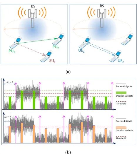
Focusing on the non-coordinated and asynchronous scenar-ios, the combination of dynamic spectrum sharing (DSS) and D2D, known as cognitive D2D (C-D2D), is considered in this paper, and a potential paradigm for future D2D communica-tions is studied. The major advantages of C-D2D are two-fold. First, the spectrum scarcity, worsened by the emerging ultra-dense networks, will be alleviated by opportunistically accessing spectrum in proximity [13], [14]. Recently, LTE in unlicensed band (LTE-U) opens a wide perspective for DSS-based commercial communications. Second, a listen-before-talk (LBT) technique provides a natural tool of interference mitigation, by excluding the coordination from BS. Thus, the listening to unknown wireless environments, e.g. detecting or discovering active device, will be of great importance to C-D2D [10], [15], [16]. Note that, in the context of C-C-D2D, the device discovery and spectrum detection may have the same formulation, i.e. directly identifying whether there are signals on the specific band and, if possible, estimating what the associated link information states (LSI) are, see Fig. 1-a. For asynchronous C-D2D communications, direct device discovery/detection [17], which will be implemented in ablind
manner [18], thereby requires in essence two functions: the existence detection and the LSI acquisition.
be unknown. So, it is unable to determine a proper decision threshold for detection. For another, the wireless environment may also change dynamically [23], [24], which renders the fading channel time-dependent and arouses additional informa-tion uncertainty in decision process, further deteriorating the detection performance. Whilst the fixed-threshold technique may be used (e.g. relying on a Neyman-Pearson criterion), it would noticeably degrade the performance, by causing the high miss detection (as illustrated by Fig. 1-b) and thereby the harmful interferences to primary transmission. Another expedient approach is to marginalize such uncertain states (e.g. dynamical channel or timing drift) [21] or exploiting their expectation as one practical alternative, which achieves less competitive performance.
Thesecondobjective, the acquisition of LSI will be of great significance to C-D2D communications [25], which should be estimated in real-time, in order to improve detection perfor-mance and optimize subsequent transmission. For example, except for promoting device detection, accurate timing is required in the hand-shake of two devices in proximity, whilst channel gains are critical to power control and mode selection (if the network involvement is available) [10], [31]. However, in out-of-coverage situations the acquisition of such LSI must be realized blindly, at the same time of detecting unassociated device. The involved two-level interruptions, i.e. (1) the mutual influence in estimating unknown timing and channel gains, and (2) the mutual interruption between detection and estimation as well as the resulting error propagation, will make most Bayesian schemes invalid.
In this study, a novel asynchronous device detection paradig-m is proposed for C-D2D coparadig-mparadig-munications, whereby the centralised coordination tend to be not practical. To be specific, we formulated the challenging task as one track-before-detect (TBD) problem, as known in the target-tracking literature [26]–[28]. In contrast to conventional sensing approaches where the signal is first detected, and then the signal is estimated, our new scheme jointly accomplishes detection and estimation in order to make use of all statistic information available in received signals. To do so, rather than a classical two-hypothesis test (THT) formulation, we adopted another new concept of random finite set (RFS). By unifying the binary existence of target signals and the associated state of object as one generalized random variable, RFS has become one pow-erful analysis tool to deal with object tracking problems [24], [25], [27], [29], [30], [42]. To sum up, the main contributions are summarized as follows.
1. We consider two inherent difficulties in C-D2D device detection, and thereby formulate a general dynamical system model. Both evolving timing drifts and time-dependent fading channels are cast into the model. Such two information uncer-tainties, which are characterized respectively by two random processes, are viewed as two hidden states to be estimated.
2. We find multipleheterogeneousrandom variables render the algorithm design a tough work. Specifically, the device de-tection concerns an unknown binary variable (i.e. “1” for active or “0” for sleep), whilst the estimation of timing drifts and fading channels is associated with another high-dimensional discrete space. Meanwhile, the timing drift is input-dependent,
(a)
[image:3.612.320.553.50.312.2]
(b)
Fig. 1. (a)Left: The spectrum detection is performed by a secondary user, while the two primary users are communicating with each other.Right: The device discovery is realized among two UEs. (b)Top: The synchronization between the unassociated device and the D2D devices is accomplished. Bottom: The dynamic timing drift exists among two unassociated devices.
while the channel fading is input-independent. Another major challenge is that the detection and estimation process will be coupled mutually. To combat this, we treat the mixed detection and estimation (MDE) process as one generalized estimation problem, and formulate the heterogeneous variables as one Bernoulli RFS.
3. We propose a flexible algorithm relying on Bayesian statistical inference, which accomplishes the devices detection (or spectrum sensing) and, at the same time, acquires two dynamical LSI. To address the MDE problem, which is prob-ably beyond the capacity of classical estimation techniques, the designed scheme is based essentially on a sequential maximum
a posteriori (MAP) criterion. Simplified implementation of the recursive estimation is then investigated, by resorting to a sequential importance sampling (SIS) technique.
4. We evaluate the detection/estimation performance in the presence of dynamical timing drift and time-dependent fading channel. It is demonstrated via simulation that, using our new algorithm, both two unknown LSI will be tracked accurately. The information uncertainty, therefore, can be reduced to the maximum, and the detection performance will be promoted. By alleviating the inflexible requirement on coordinated timing or pilot signaling, the proposed scheme will show the great promise to future C-D2D communications, by facilitating the spectrum-efficient and proximity-inspired transmissions.
estimates time-varying LSI and device state is proposed, by presenting a flexible Bernoulli filtering scheme. In Section IV, numerical results and performance analysis are provided. Finally, we conclude this investigation in Section V.
II. SYSTEMMODEL
In this paper, we consider a distributed D2D communication network, which employs dynamic spectrum access. The main motivations will be two aspects. First, a cluster-header is usually resource-demanding and becomes the network bottle-neck in terms of energy and longevity [1], [32]. Second, a centralized control relies on frequent information exchanges, which becomes even impractical in adverse environments.
In C-D2D, the device discovery, or spectrum sensing, share the same problem formulation, as illustrated in Fig. 1-(a). For spectrum sensing, a PU device will occupy a frequency band, while the SU manages to identify whether this band is occupied and utilizes a DSS strategy to avoid interference. If the band is unoccupied, a SU will access and talk with another proximity device; otherwise, it will sense another band [20], [23]. For direct device detection, a UE will sense the specific channel to find one potential device in proximity for data transmission. This process is also blind, in the case of out-of-coverage D2D scenario, as in spectrum sensing. More importantly, except for the similar objective, the unknown LSI involved in above two processes are almost the same.
(1) Due to the lack of centralized coordination, the timing information among two unassociated devices will be unavail-able. To this end, as illustrated in Fig. 1-(b), a detection slot may be deviated from the emission slot of another device. Thus, the statistical likelihood of decision variable will become unknown and the detection performance will be deteriorated remarkably, as a decision threshold is associated with with varying timing drifts.
(2) Meanwhile, given dynamical wireless environments (e.g. aroused by device mobility), the channel gain for a particular frequency will be time-dependent, by introducing random fluctuations in received signals. Combined with the timing drifts, the resulting serious information uncertainty poses formidable challenges to accurate device detection/discovery in asynchronous C-D2D scenarios.
A. Dynamic State-Space Model
For the device detection in C-D2D communications, a new dynamical system model is established, i.e.,
sn=S(sn−1), (1)
Mn=T(Mn−1, un), (2)
αn=H(αn−1), (3)
zn=Z(tn, αn, sn,{wn,m}Mm=1). (4)
Here, Eqs. (1)-(3) are referred as to dynamic equations, which respectively describe the stochastic transitions (from discrete time n−1 to time n) of unknown states, i.e., the existence statesn, the discrete timing driftMnand the fading
gainαn. Eq. (4) is themeasurementequation, which specifies
the coupling relationship between unknown states (Mn,αn)
and the observationzn at timen.
B. Dynamics of PU States
The first stochastic function S(·) : Z1 7→ Z1 specifies
the dynamical behavior of device states at the nth time. To be specific, sn=1 indicates the existence of an active
device, while sn=0 represents the absence of active device.
Here, it is modeled as one 1st-order Markov process, i.e. sn ∈ S , {0,1} [33], [34]. Accordingly, its transitional
probability matrix (TPM) is given by:
P=
1−pb pb
1−ps ps
, (5)
whereps denotes the survival probability, i.e., the probability
of a PU stays in an active stateS1and also inS1at the
previ-ous slot and the current slot, i.e.,ps:=Pr{sn+1= 1|sn= 1}.
pb is the birth probability, i.e., the probability a PU keeps
inactive state inS0 at the previous slot and switches to S1 at
the current slotn,pb:=Pr{sn+1= 1|sn= 0}.
Given the prior TPM, the inexplicit dynamic function S(sn−1)will be determined via:
Pr{S(sn−1) =sn}=Pr{sn−1|sn}, sn ∈ S. (6)
C. Dynamics of Channel Fading
The dynamical function H(·) : R1 7→ R1 characterizes the transition of channel fading αn ∈ A (A ⊂ R1). Note
that, here we focus on the fading gain (as required by the non-coherent observation and the mode selection application when roughly evaluating SNRs), which is modeled as one discrete-state Markov chain (DSMC) [35]–[37]. Different from the other auto-regressive (AR) model, the stochastic dynamic function H(αn−1) will be determined by a group of
transi-tional probabilities, i.e.,
Pr{H(αn−1) =αn}= Πk→k0, αn−1, αn∈ A.
Here, each transitional termΠk→k0 defines the probability
of a fading stateαn, switching from the statekat time index
(n0−1) to the statek0 at time indexn0, i.e.,
Πk→k0 ,Pr(αn0 =Ak0|αn0−1=Ak). (7)
For the slowly evolving fading, the transitional time is denoted as n0 = bn/Lc [23], [35], where L is the static length in which the fading gain αn will remain unchanged
temporarily. Taking the Rayleigh fading of|A|=Kstates for example, i.e.f(αn) = ασ2n
α
×exp(−α2n
2σ2
α
),Πi→j will be derived
via:
Πk→k0 ,Pr({αn0 ∈[vk0, vk0+1)|αn0 ∈[vk, vk+1)},
= 1 πk
Z vk0+1
vk0
Z vk+1
vk
f(αn0−1, αn0)dαn0−1dαn0, (8)
where f(αn0−1, αn0) is the bivariate Rayleigh joint
prob-ability density function (PDF) [38], and 0 ≤ k, k0 ≤
|A| − 1. The partitioning bounds vk will divide
chan-nel gain into K non-overlapped regions. Using an equi-probable partition rule, i.e. with K equivalent steady probabilities πk =
Rvk+1
vk f(αn)dαn = 1/K, we have
vk =
−2σα2×ln(1−k/K)
1/2
, and Ak =
Rvk+1
f(αn)dαn [35], [36]. Here, the first-order DSMC is used,
which is sufficient to characterize slow-varying fading chan-nels [23], [35]. Thus, the fading states are related only with its immediate neighborhood states, i.e. Θk→k0 = 0 for |k− k0| > 1. Accordingly, the TPM of fading channels, denoted byΠΠΠK×K={Πk→k0}, k, k0∈ {0,1,· · ·, K−1}, is
expressed as Eq. (9).
D. Dynamic of timing deviations
We consider two different types of timing drifts.
(1) Case 1: Uncorrelated drifting In the first case, the
transmission interval of different slots is independent of each other, i.e., E{(tn −tn−1)·(tn−1−tn−2)} = 0. Given the
detection slotTf and the sampling frequencyfs, there contain
M =bTf/fs]samples in each slot. As far as discrete samples
are concerned, the deviated samples Mn aroused by timing
drifts will be ranged in M,[0, M−1], and accordingly, in each slot there contains only (M−Mn)informative samples.
In order to determine the statistical distribution of Mn,
assume the interval between two transmissions follow the iden-tically and independently (i.i.d) exponential distributionE(λ), i.e. Pr{tn−tn−1}∼λ·exp{−λ(tn−tn−1)}. Given the initial
condition t0=0 and each emission intervalV(n),tn−tn−1,
the nth transmission time will be tn =P n
l=1V(l), and the
resulting deviationt∆(n)is:
t∆(n) =mod
hXn
l=1V(l), Tf
i
∈(0, Tf], (10)
wheremod[a, b]gives the modulo operation onawith regards tob. For the discrete samples, a similar relation holds, i.e.,
Mn=mod
hXn
l=1V∆(l), M
i
∈ M, (11a)
V∆(n) =b(tn−tn−1)/Tfc, (11b)
and the i.i.d random variable V∆(n) is also exponentially
distributed, i.e.V∆(n)∼E(λ∆), withλ∆=bλ/Tfc. Moving
on, we obtain the following equivalent relation, i.e.,
Mn =mod
nXn
l=1mod[V∆(l), M], M
o
,
=modhX
n
l=1Yl, M
i
, Yl∈ M. (12)
It is noted that Yl , mod[V∆(l), M] is also an i.i.d
random variable, with a discrete PDF specified by a group of probability mass {wm}(m∈ M), i.e.,
p(Yn) =
M−1
X
m=0
wm×δ(Yn−m), (13)
wm=
∞
X
k=0
λ∆×exp[−λ∆(m+kM)]. (14)
-100 -80 -60 -40 -20 0 20 40 60 80 100 10-4
10-3
Deviated samples
PD
F Simulation
[image:5.612.324.549.49.225.2]Uniform distribution
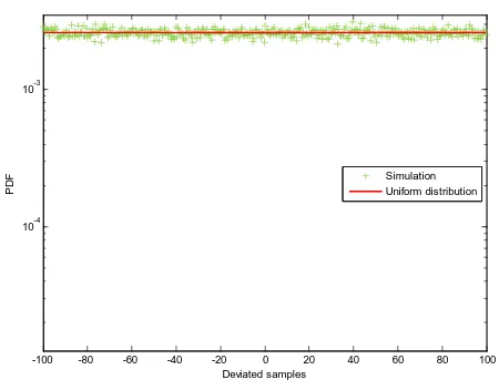
Fig. 2. The distribution of random timing deviations in the case of uncorrelated emission intervals. Each transmission interval is i.i.d distributed according to the negative exponential density ofλd= 10. The sample length
isM= 200.
For the above modulo operation, the central limits theorem (CLT) formodulo 1will be directly applied [39]. I.e., for the i.i.d variableYn ∈[0, M−1]the modulo on the summation
of Yn will converge weakly to auniform distribution, i.e.,
modhX
n
l=1Yl, M
in→∞
−→ U(0, M), (15)
subject to the condition
lim
n→∞p(Y1)p(Y2)· · ·p(Yn) = 0.
We then show that, for the above considered case, the term
∆n ,p(Y1)p(Y2)· · ·p(Yn)satisfies
∆n= n
Y
l=0
M−1
X
m=1
∞
X
k=1
λ∆×exp{−λ∆[m+kM]},
<
n
Y
l=0
M−1
X
m=1
λ∆×exp{−λ∆·m},
<
n
Y
l=0
λ∆×exp{−λ∆}=λn∆×exp(−nλ∆)
n→∞
−→ 0.
Thus, relying on the modulo-CLT, the deviated samples Mn in uncorrelated cases will be distributed according to
U(0, M), as further verified by Fig. 2. So, the transitional functionT(tn−1)will be given as:
Pr{T(tn−1|tn−1)}=Pr{T(tn−1)}= 1/M. (16)
(2) Case 2: Correlated drifting With correlated
trans-mission intervals, the etrans-mission interval of the nth time will become correlated with the previous (n − 1)th slot, i.e.
Π Π ΠK×K=
Π0→0 Π0→1 0 0 · · · 0 0 0
Π1→0 Π1→1 Π1→2 0· · · 0 0 0
..
. ... ... ... . .. ... ... ...
0 0 0 0 · · · Π(K−2)→(K−3) Π(K−2)→(K−2) Π(K−2)→(K−1)
0 0 0 0 · · · 0 Π(K−1)→(K−2) Π(K−1)→(K−1)
E{(tn −tn−1)(tn−1−tn−2)} 6= 0. In this case, the
statis-tical distribution of timing drifts will be hardly derived, and alternatively, we use a general Gaussian model to describe the stochastic procedure, i.e.,
tn =tn−1+τn,
where the driven termτnis assumed to follow an i.i.d Gaussian
process [40], with the zero mean and the variance σ2τ. It is found that, for the discrete samples, the samples deviationMn
will be characterized by:
Mn =Mn−1+ ∆n, (17)
where the discrete driven term ∆n accordingly follows a
discrete Gaussian processNd(0, σ∆2).
It should be notworthy that, as far as the real timing tn is
concerned, the resulting deviationMnwill be always positive.
For the convenience of analysis, yet we will consider the discrete deviationMnis equivalently ranged in[−M/2, M/2].
That is, a negative Mn accounts for the advanced drift, i.e.,
theMn deviated samples fall into the previous(n−1)th slot;
whilst a positive Mn indicates the delayed drifting and Mn
samples fall to the next (n+ 1)th slot. Of course, the other equivalent formulationMn∈[−M, M]can be also applicable,
and the designed algorithm is independent of specific prior information. As such, we have:
Pr{Mn|Mn−1} (18)
=
(
1.q2πσ2
∆·exp[−(Mn−Mn−1)2/2σ∆2], case1,
U(−M/2, M/2], case2.
E. Observation
The observationzn∈ Z(Z ⊂R1)at the nth detection slot
will be calculated via:
zn = M
X
m=1
n
αncn(m)δ(sn−1)GMn(m) +wn(m)
o2
, (19)
=
M
X
m=1
n
αncn(m)GMn(m) +wn(m)
o2
, sn= 1,
M
X
m=1
w2n(m), sn = 0.
Here,δ(x)denotes a Dirichlet function, which indicates the existence of the target signal; GMn(m) (m = 1,2,· · ·, M)
accounts for a window function imposed on target signals, which is aroused by timing driftsMn.H0andH1 correspond
to two hypotheses, respectively, i.e., the absence and presence of target signals cn(m) = bn(m) ×p(m), where bn(m)
represent the unknown information symbols, and p(m) is the pulse-shaping response. For simplicity, the binary phase shift keying (BPSK) signal is considered, i.e. bn(m)∈ B =
{√Es,−
√
Es} with EB{b2n(m)} = Es. The noise samples
wn(m) ∈ R1 are assumed to be zero-mean additive white
Gaussian noise (AWGN) which is independent of other hidden states, i.e., wn(m) ∼ N (0, σw2). When the non-coherent
observations are concerned [23], [24], the generalization of the
model and subsequent algorithm to other unknown modulated signals will be straightforward.
Note that, when Mn=0 we have GMn(m) = 1 for m =
1,· · ·, M. For the positive Mn > 0, the window function
GMn(m)will be specified by:
GMn(m) =
0, 1≤m≤M
n, (20a)
1, Mn+ 16m≤M, (20b)
and for a negativeMn<0, we have
GMn(m) =
1, 1≤m≤M− |Mn|, (21a)
0, M− |Mn|+ 1≤m≤M. (21b)
Considering a caseMn>0, two pieces of summed energy
will be calculated respectively, i.e.,
zn(1) =
Mn
X
m=1
w2n(m), zn(2) = M
X
m=Mn+1
[αncn(m)+wn(m)]2.
It is found that such two components will be independent of each other. Given independent noise samples, the likelihood functionp{zn|αn, sn = 1, Mn}is evaluated viap{zn(1)|sn=
1, Mn} ×p{zn(2)|αn, sn = 1, Mn}. Here, p{zn(1)|sn =
1, Mn} follows the central Chi-square distribution of the degree Mn, while p{zn(2)|αn, sn = 1, Mn} follows a
non-central Chi-square density of the degree (M −Mn) with a
non-central parameter[M −Mn]·E{c2n(m)}α 2
n/σ
2 w.
When bothM−Mn andMn are sufficiently large (>20),
then each component (zn(1) or zn(2)) follows the Gaussian
distributions, according to the CLT. Given different emission status of unassociated devices (i.e. sn) as well as the related
LSI (i.e., αn andMn), the approximated likelihood
distribu-tions will be:
ϕn(zn|sn= 0) =N {M σw2,4M σ 4
w}, (22)
ϕn(zn|αn, sn = 1, Mn) =
N {E{zn(1)|sn= 1, Mn},V{zn(1)|sn= 1, Mn}} ×
N {E{zn(2)|sn= 1, Mn},V{zn(2)|sn= 1, Mn}}. (23)
where each single mean and variance terms, in the case of sn=1, will be given by:
E{zn(1)|sn = 1, Mn>0}=Mnσw2, V{zn(1)|sn= 1, Mn >0}= 4Mnσ4w,
E{zn(2)|αn, sn= 1, Mn >0}= 2(M−Mn)Esα2nσ 2 w, V{zn(2)|αn, sn= 1, Mn>0}= 2(M−Mn)Esα2nσ
2 w
+ 4(M −Mn)σ4w.
III. ASYNCHRONOUSDEVICEDETECTION
To implement the mixed device detection and LSI es-timation in the context of unknown timing, we adopt the maximuma posteriori(MAP) criterion and design a stochastic filtering scheme. Rather than relying on a fixed threshold, we manage to exploiting fully the dynamical statistics involved in the received signals. Our new scheme is thereby rooted on a Bayesian rule, which is committed to estimate the joint posterior density, i.e.,
( ˆαn,sˆn,Mˆn) = arg max
αn∈A,sn∈S,Mn∈M
p(α1:n, s1:n, M1:n|z1:n),
wheres1:n={s1, s2,· · · , sn} denotes the trajectory of
trans-mission states until the nth slot, while α1:n, M1:n and z1:n
are three trajectories of fading gains, varying timing drifts and observations, respectively. It is noteworthy that, relying on a concept of THT, the Neyman-Pearson (NP) criterion becomes inadequate to the new formulation of joint estimation [34].
A basic idea here is the recursive estimation, which exploits the underlying dynamics of unknown states. That mean-s, a sequential Bayesian framework, i.e., predict using the Chapman-Kolmogorov (CK) equation and then updating with the Bayesian rule, will be adopted. A major difficulty is that, unlike the tracking of an established link channel, the likelihood density will be unavailable due to the random presence/absence of device. Therefore, the formulated MDE problem in Eq. (24) still remains a substantial challenge.
In the section, we suggest a new formulation to charac-terize the stochastic presence of device and the dynamics of its related LSI (i.e. the varying timing drift and channel fading). Then, for the specific application we further design a sequential estimation scheme.
A. Random Finite Set
We formulate a Bernoulli RFS (BRFS)FFFn to characterize asynchronous device detection with unknown LSI. To be specific, the BRFS cardinality of time n, which is denoted
bydn=|FFFn|(d∈N0={0,1,· · · })and follows a Bernoulli
distribution κ(d) = Pr{|FFFn| = d} [29], [30], [41], is used
to indicate whether an device is transmitting signal or not. Meanwhile, a compound state fn ,{Mn, αn} ∈ A × M ⊂ R2, related with an unassociated device, consists of unknown
timing drifts and fading gains, which evolves with time. Thus, an RFS FFFn is able to cast two-level uncertainties into one random process, i.e., whether there are target signals and what its related LSI is.
In following analysis, we adopt the Mahler’s approach to define the finite set statistics (FISST) PDF ofFFFn [29], i.e.,
p(FFFn={f1,f2,· · ·,fd}) =n!κ(dn)·p({f1,f2,· · ·,fd}).(25)
In the context of the set integral operation R
p(FFFn)dFFFn
(rather than the distribution integration),p(FFFn)can be viewed as one PDF, i.e., R
p(FFFn)δFFFn =p(FFFn =∅) + [1−p(FFFn= ∅)]×R p(fn)dfn= 1. For the considered BRFS, i.e.,|FFFn|=1, the above FISST PDFp(FFFn)is rewritten to:
p(FFFn) =
1−q
n, ifFFFn =∅, (26a) qn×p({Mn, αn}), ifFFFn={Mn, αn}. (26b)
Note that, for the cases dn >1 we will have p(FFFn)=0. In
other words, in a Bernoulli RFS an unassociated device is either active (e.g. with a probability of qn) or inactive (e.g.
with a probability of1−qn) [42]. Accordingly, the cardinality
density is specified as:
κ(d) =
1−q
n, ifFFFn=∅, (27a) qn, ifFFFn={Mn, αn}. (27b)
B. Sequential MAP
Using the Bayesian sequential inference, the transitional densities of unknown states as well as the likelihood on new observation will be fully utilized. Thus, a two-stage recursive procedure will be implemented, i.e.
pn|n−1(FFFn|y1:n−1) =
Z
F F Fn−1
φn|n−1(FFFn|FFnF −1)×pn−1|n−1(FFFn−1|y1:n−1)dFFFn−1,
(28)
pn|n(FFFn|yz1:n) =
ϕn(yn|FFFn)pn|n−1(FFFn|y1:n−1)
R
F F
Fnϕn(yn|FFFn)pn|n−1(FFFn|y1:n−1)dFFFn
.
(29)
As mentioned, the one-step prediction of Eq. (28) mainly utilizes the prior traditional information and a C-K equa-tion [43]. The updating stage in Eq. (29) relies on a Bayesian rule, by fully exploiting the real-time information carried with the new observation. Compared to classical Bayesian estimation methods, notable difference in the RFS inference is that, rather than the distribution integration, the set integral operations (i.e.δFFFn) will be used.
Recalling the previous Markov models, the transitional den-sity of our formulated BRFS, i.e.,φn|n−1(FFFn|FFFn−1), will be
characterized by also a 1st-order Markov process. Conditioned on different feasible states at the timen-1, we have:
φn|n−1(FFFn|∅) =
1−p
b, ifFFFn=∅,(30a) pb·bn|n−1({Mn, αn}), else, (30b)
and
φn|n−1(FFFn|fn−1) =
1−p
s, ifFFFn=∅, (31a) ps·pn|n−1(fn|fn−1), else. (31b)
Here, the a priori density bn|n−1({Mn, αn}) specifies an
initial distribution for a singleton state |FFFn| = 1, if one unassociated device that does not exist at timen-1 is appeared at the timen, i.e.bn|n−1({Mn, αn}) =Pr{{Mn, αn}|qn−1=
0}, as discussed shortly.
C. Bernoulli Filtering
The above sequential estimation, in the context of random absence of target signals, remain relatively different from classical Bayesian estimation, e.g. the Kalman filtering [37]. In sharp contrast, two coupled posterior densities need to be estimated jointly, in order to determine the FISST PDF pn|n(FFFn|z1:n) in Eq. (26). The first one, referred as to
the existence density, indicates whether the target signal is contained in received samples, i.e.,
qn|n,Pr(|FFFn|= 1, sn = 1|z1:n), (32)
The second one is used to characterize the related LSI (e.g. unknown timing drifts and fading gains) when an unassociated device is active at time n, which is also known as the a posteriorispatial PDF, i.e.,
Solving the above RFS inference process will be premised on a similar two-stage process. In the first stage, the above two densities will be predicted relying on the prior transitional densities as well as the posterior densities of previous time n−1. In the second stage, such two predicted densities will be updated by further exploiting the current observation.
1) Prediction Stage: With the help of C-K equation, the 1st-order prediction process will be realized. Given the posterior density of timen−1, i.e.qn−1|n−1andpn−1|n−1(fn), two
pre-dicted distributions of the timen, i.e.,qn|n−1 andpn|n−1(fn),
will be derived respectively from Eqs. (34) and (35): (see the bottom of the next Page):
qn|n−1=pb×(1−qn−1|n−1) +ps×qn−1|n−1. (34)
The similar derivation procedure of two above equations may be found in some previous works [25], [34], [42]. The expressions of such two densities are relatively easy to follow. Each predicated density will be contributed by two
complimentary terms, i.e., the component from a sustained active device (i.e. which is related with qn−1|n−1 and known
as thesurvivalcomponent), and the other component from the newly birthed device (i.e. which is related with1−qn−1|n−1
and refereed as to thebirth component).
2) Update Stage: Relying on the new observation zn, the
predicted densities attained by the first-stage will be updated. The updated densities, by incorporating the innovation infor-mation, will be more accurate, which are given by Eq. (36) (at the bottom of the page) and
pn|n({Mn, αn})
=R rn(zn|{Mn, αn})×pn|n−1({Mn, αn})
A,Mrn(zn|{Mn, αn})×pn|n−1({Mn, αn})dαndMn
,
(37)
where the likelihood ratio is defined as:
rn(zn|{Mn, αn}) =ϕn(zn|αn, sn= 1, Mn)/ϕn(zn|sn= 0).
(38)
With the derived two posterior densities, the unassociated device will be detected via the MAP criterion, i.e.,
ˆ sn =
1, ifq
n|n> γ, (39a)
0, ifqn|n≤γ, (39b)
where γ will be configured to 1/2 as in a Bayesian rule. Meanwhile, the unknown LSI will be estimated via:
{Mˆn,αˆn}= arg max
Mn∈M,αn∈A
pn|n({Mn, αn}). (40)
3) Related Densities: In the analysis, the prior transitional density of dynamical timing drifts will be determined via E-q. (41), which will be dependent of various emission intervals.
pn|n−1({αn, Mn}|{αn−1, Mn−1})
=Pr(α0n=Ak0|αn0−1=Ak)×Pr(Mn|Mn†) (41)
=
Π
k→k0·N(Mn−Mn†; 0, σ2∆), Type1,
Πk→k0·U (Mn−Mn†; [−M/2, M/2]), Type2.
Notice that, n† denotes the previous time slot of
unassoci-ated emission. It is noteworthy that this previous emission slot n†may be smaller thann−1. I.e. such anemission-dependent
dynamical process will be different from that of fading gain, which is closely related with PU’s emission states. In other words, the timing driftMn is not necessary to estimate in the
case of sn = 0 and, in contrast, the fading channel needs to
be estimated even ifsn=0. To be specific, if an unassociated
device is active at time n−1, then the estimated fading state is αˆn−1 = ˆαn−2 in the case of mod(n−1, L) > 0
and sn−1 = 0; otherwise, it will be estimated via the prior
transitional densityαˆn−1 = arg max αn−1∈A
p(αn−1|αˆn−2)in the
case of mod(n−1, L) = 0andsn−1= 0.
It is seen from the predict-update procedure that the pro-posed scheme can effectively address the aforementioned like-lihood disappearance and the mutual interruption problems. First, the combination of birth and survival components, see Eq. (34) and (35), as the expectation on the corresponding densities, would cope with the influence from the existence
uncertainty (sn = 1 or sn = 0). Second, the mutual
inter-ruption is fully embodied by two coupled densities, i.e., the existence density and the spatial density, which can be now estimated jointly.
As mentioned, the birth density will be of importance to sequential estimation, which should be properly designed. In this work, the birth density is specified as in Eq. (42), given the independent timing drift and channel fading, i.e.,
bn|n−1({Mn, αn}) =bn|n−1(αn)×bn|n−1(Mn). (42)
For the fading gain, a birth sub-density is assigned as:
bn|n−1(αn) =Pr{αn|sn−1= 0}, (43)
=
Z
A
pn|n−1(αn|α˜n−1)·bn−1( ˜αn−1)d˜αn−1,
where the termα˜n−1is viewed as an intermediate state, which
is derived from the estimated fading state of previous time
pn|n−1({Mn, αn}) =
pb·(1−qn−1|n−1)×bn|n−1(Mn, αn)
qn|n−1
+
ps·qn−1|n−1×
R
A,Mpn|n−1({Mn, αn}|{Mn−1, αn−1})·pn−1|n−1({Mn, αn})dαndMn
qn|n−1
. (35)
qn|n=
qn|n−1×
R
A,Mrn(zn|{Mn, αn})·pn|n−1({Mn, αn})dαndMn
1−qn|n−1+qn|n−1×
R
A,Mrn(zn|{Mn, αn})·pn|n−1({Mn, αn})dαndMn
n−1. Given the estimation stateαˆn−1, we have:
bn−1( ˜αn−1=Hj) =
1/3, αˆ
n−1=Hi &|i−j| ≤1,
0, αˆn−1=Hi &|i−j|>1.
For the timing drift, its birth sub-density is specified by:
bn|n−1(Mn) =Pr(Mn|z1:n−1),
'pn|n−1(Mn|Mˆn†). (44)
D. Implementations
Although the recursive propagation of posterior densities provides a theoretic framework for the BRFS estimation, the involved computation complexity will be very high. I.e., when the sample sizeM is large, then the state space of timing drifts will be enlarged. Considering the fading gains, the unknown state space will becomeK×Mdimensional, rendering a direct computation/integration infeasible. To alleviate the difficulty, particle filtering (PF) is used to implement the Bayesian inference via a simulated Monte-Carlo approach [44], relying on the sequential importance sampling (SIS).
1) PF: Using the PF, a group of discrete particlesx(ni)with
evolving probability mass (or weights)w(ni) (i= 1,2,· · ·, I),
which are simulated from a proposal density, i.e., x(ni) ∼ π(x(ni)|z1:n), are employed to approximate complex integration
via numerical summation [44]. That is, the involved density pn(xn)will be computed via:
pn(xn) = I−1
X
i=0
w(ni)×δ(x−x(ni)), (45)
where the compound state is xn , {Mn, αn}. Thus, the
essence of PF is to design a proper proposal density, from which we can (1) sample I discrete particles, and (2) update the particle weights recursively. In general, given a proposal densityπx(ni)|z1:n
, the particle weighsw(ni)are updated by:
w(ni)=w(ni−)1×
pzn|x(ni)
·px(ni)|x
(i)
n−1
πx(ni)|x1:n−1, z1:n
. (46)
2) Bernoulli PF: As far as Bernoulli PF (BPF) is con-cerned, we need to approximate the predicted spatial density via pˆn|n−1(x) ' P
I−1
i=0 w
(i)
n|n−1 × δ
x−x(ni|)n−1. Given two complementary components (i.e., survival and birth), a group of discrete particles are sampled from a piece-wise distribution [25], [42], i.e.,
x(ni|)n−1∼
(
ξn
xn|n−1|x
(i)
n−1|n−1, z1:n−1
, i= 1,· · ·, J,(47a)
βn(xn|n−1|z1:n−1), i=J+ 1,· · · , J+B. (47b)
where the firstJ particles will approximate the survival term, whilst the laterB particles are used to evaluate the birth term. Then, the associative weights evolve according to:
w(ni|)n−1= (48)
ps·qn−1|n−1
qn|n−1 ·
pn
xn(i|)n−1|xn(i−)1|n−1
ξn
xn|n−1|x
(i)
n−1|n−1, z1:n−1
·w
(i)
n−1|n−1,
i= 1,2,· · ·, J,
pb×(1−qn−1|n−1)
qn|n−1
×
bn|n−1
x(ni|)n−1
B×βn(xn|n−1|z1:n−1)
,
i=J+ 1,· · ·, J+B.
Usually, in order to eliminate particles with extremely small weights, a re-sample process will be adopted if necessary [45].
3) Proposal survival-density: The proposal density, related with the survival component, will be determined recursively. I.e., with the predict particles and weights of the previous time n−2, the posterior density of timen−1will be approached after updatingJ +B particle weights. Thus, J new particles can be simulated from the updated posterior density at time n−1, i.e.,
x(ni−)1|n−1∼ J+B
X
i=1
δx−xn(i−)1|n−2×
ϕn
zn−1|x
(i)
n−1|n−2
·wn(i−)1|n−2, (49)
These J particles x(ni−)1|n−1 (i = 1,· · ·, J), as survival particles, will be retained for the subsequent timen.
4) Proposal birth-density: The proposal birth density will be assigned directly as thea prioritransitional density, i.e.,
x(ni|)n−1∼bn|n−1(αn)×bn|n−1(Mn|z1:n−1). (50)
Premised on a PF approach, the predicted spatial density pn|n−1(x), which involves theK×M dimensional space, will
be approximated via:
Z
A,M
rn(zn|{Mn, αn})·pn|n−1({Mn, αn})dMndαn,
' J+B
X
i=1
rn
zn|x
(i)
n|n−1
×w(ni|)n−1. (51)
5) Practical Considerations: As the fading channel αn
will keep temporarily invariant within L successive slots, the observations within such a static length (in the case of qn|n > γ) can be accumulated, which further improves
the degree of likelihood density and thereby promotes the estimation performance. Besides, in order to reduce the popu-lation of particles when sampling from aK×M dimensional space,Iparticles are employed to respectively simulate fading states and timing drifts, and then I compound particles of 2-dimensional is formulated by binding them together.
An schematic flow of the proposed algorithm is summarized
inAlgorithm. 1. (1) Provided the current observationzn, the
posterior existence probability qn|n and the spatial density
pn|n(Mn, αn)are estimated, by using a two-stage (prediction
and update) procedure; (2) in the case ofqn|n > γ, the
obser-vation will be accumulated to further promote the accuracy of likelihood; (3) the unknown device as well as its associated LSI will be estimated by maximizing the posterior densities.
(1) O(M) multiplications are required when constructing the summed-energy observation. (2) In subsequent BPF, the required multiplications are basically proportional to the size of used particles I. Here, ϑ denotes the required multiplica-tions when processing each particles, including the transitional operation and likelihood evaluation.
As demonstrated by Eq. (46) and (48), the main computation of our algorithm comes from the evaluation of Gaussian likeli-hood function forI independent particlesx(ni), accompanying
M power operations. We assume a configuration of M=200 andI=100, and use a single core of anARM Cortex A9(which is not a cutting-edge, as far as the next-generation smart-phone is concerned) to implement the involved computation. We found the algorithm will take less than 0.1 millisecond-s (i.e. the real-time float-point computation). Reducing the sample size M and particle size I directly may lead to the simplified complexity, yet there involves a practical compro-mise between performance and complexity1. For the typical sensing-transmission frame length of 20∼100 milliseconds, therefore, the time-delay will be basically negligible. Also, if further considering the resource-efficient automatic generation of look-up-table [47], the power consumption is not really a big cost when implementing the algorithm locally (around 10 times per second in detection stage).
IV. NUMERICAL SIMULATIONS
In the section, the performance of the proposed algorithm will be evaluated via numerical simulations. In order to mea-sure the detection performance, theright detection ratioPDis
adopted as a performance metric as in refs. [23], [34], which takes both the miss detection probability Pm and the false
alarm Pf into considerations and, therefore, is more suitable
to the designed Bayesian scheme.
PD= 1−p(H1)Pm−p(H0)Pf. (52)
For time-dependent fading channels, the mean square error (MSE) of estimations will be evaluated, i.e.
MSEα,
1 N ×E
XN
n=1|αˆn−αn|
2/
|αn|2
. (53)
For the other important LSI, i.e. the varying timing drifts, the MSE will be calculated, i.e.
MSEt,
1 N ×E
XN
n=1|
ˆ
Mn−Mn|2/|Mn|2
. (54)
In the first simulation, the representative states of fading channel are K=7 and the variance of Rayleigh fading is σα2 = 0.5; the static length is L=20. The sample size is
M=100. The birth probability is pb=0.8 and the survival
probability is ps=0.2. The total particle size is I =200, i.e.
1For the sample size M, the tradeoff between sensing accuracy and transmission throughput has been investigated by Liang et.al. [46]. Here, we only refer to a compromise between detection accuracy and complexity computation. Notice that, for the concerned device detection with unknown timing drift, a larger sample sizeM was supposed to increase the accuracy of likelihood density and the detection performance. As shown by subsequent analysis, the increased uncertainty in timing drift, i.e.Mn∈[−M/2, M/2],
would degrade the detection. So, there involves another interesting compro-mise in configuringM.
Algorithm 1 Asynchronous device detections for C-D2D
Input: Observationz1:n, n= 1,· · · , N−1,
Initial densityq1|1, p1|1({M1, α1}),
Feasible fading stateA and its TPMΠΠΠK×K,
Feasible timing transitional modelMn =T(Mn−1). Output: Posterior densities qn|n, pn|n({Mn, αn}),
Existence statesn and LSI, i.e. {Mn, αn}.
? Initialize the particlesnx(1i), w1(i)o,I= 1,· · ·, J+B.
forn→1 toN do
? Calculate the predicted densityqn|n−1 via Eq. (34).
? Simulate(J+B)particlesx(ni|)n−1 from Eq. (47).
? Calculate the predicted particle weights wn(i|)n−1, and then normalize such particle weights.
? Evaluate the likelihood densityϕn(zn|{Mn, αn}, sn).
? Update the particles and their weights, and obtain
{x(ni|)n, wn(i|)n}.
? Calculate the existence density qˆn|n via Eq. (36), and
estimate the active statesˆn via Eq. (39).
? Approximate the spatial density pˆn|n({Mn, αn}) via
Eqs. (35) and (51), and estimate unknown LSI{Mn, αn}
via Eq. (40).
ifqˆn|n> γ and mod(n, L)>0 then
Accumulate the observations in[bn/Lc ×L+ 1, n];
Re-calculate the likelihood using the accumulated observations, and re-estimate fading stateαˆn.
end if
? Output the estimated state sˆn and the related LSI
{Mˆn,αˆn}.
end for
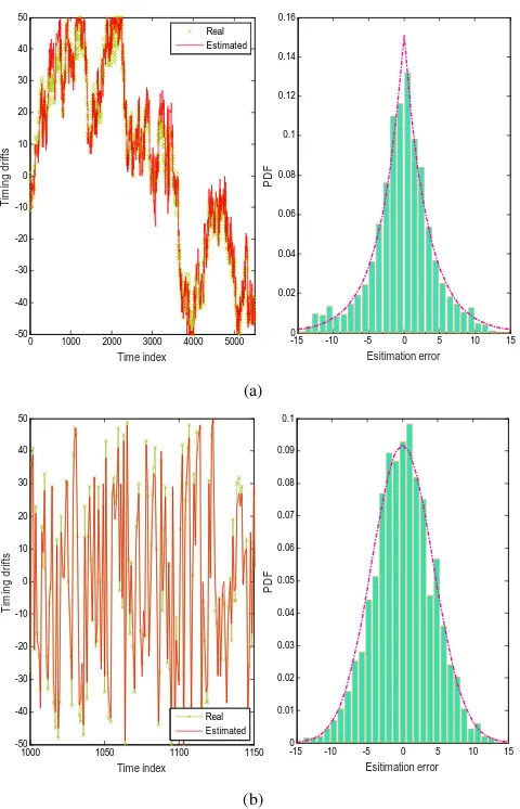
J =B = 100. We find from Fig. 3 (a)-Left, in the case of correlated transmission intervals (i.e., Type-1), the dynamical timing drifts will be varied in a correlated manner, as in Eq. (15). Using the proposed scheme, the unknown drift can be effectively tracked. From the MSE performance in Fig.
(a)-Right, the estimation of unknown timing is accurate relatively. Relying on the numerical results, the estimation error, i.e.
ˆ
Mn −Mn, will be distributed basically according to one
Laplace density, i.e. L(0,3.3). Despite the maximum devi-ation of M/2 (i.e. |Mn| ≤50 when M=100), the estimation error will never excess 15, and the mean MSE is only about 3.076 when SNR is 14dB. In Fig. 3-(b), the same observation will be made to the uncorrelated transmission intervals (i.e.
Type-2), yet with the increased estimation errors, due to the completely random timing drifts (see Fig. 3-(b)-Left).
A. Correlated timing drifts
0 1000 2000 3000 4000 5000 -50
-40 -30 -20 -10 0 10 20 30 40 50
Time index
T
im
in
g
dr
if
ts
Real Estimated
-15 -10 -5 0 5 10 15 0
0.02 0.04 0.06 0.08 0.1 0.12 0.14 0.16
Esitimation error
PD
F
(a)
1000 1050 1100 1150 -50
-40 -30 -20 -10 0 10 20 30 40 50
Time index
Ti
m
in
g
d
ri
ft
s
-15 -10 -5 0 5 10 15 0
0.01 0.02 0.03 0.04 0.05 0.06 0.07 0.08 0.09 0.1
Esitimation error
PD
F
Real Estimated
[image:11.612.56.296.49.422.2](b)
Fig. 3. (a)-Left: The estimation performance of dynamical timing drifts in the context of correlated emission intervals. (a)-RightThe estimation errors of timing drifts. In the simulation, the maximum timing drift is M=100, and the SNR is configured to 12dB. The estimation errors may follow a Laplace distribution L(0,3.3). (b)-Left The estimation performance of dynamic timing drift in the context of correlated emission intervals. (b)-Right The estimation error of the timing drifts, which follows a Gaussian distribution
N(0,4.32).
sample sizeM, the larger the uncertainty of varying timing is. Besides, given the sample sizeM, the estimation performance will be improved by an increased static length L.
The tracking performance of varying fading gains is shown in Fig. 5. We can see that, with the increasing of a static fading lengthL, the MSE performance of various sample sizes (both M=100 and M=200) will be promoted significantly. This is easy to follow. The larger the static lengthL, the more observa-tions (within a static length) will be accumulated, resulting in the more accurate likelihood information. However, it is noted that, when the sample size is M=200, the MSE of estimated fading gain will be slightly inferior to that of M=100 (when L= 20). Despite more samples ofM=200 and the increased accuracy of likelihood, the maximum timing deviations will also be increased to 100 (e.g. from 50 in the case ofM=100). As a consequence, the improved likelihood density would be compromised by the increased timing uncertainty. The theoretical analysis on proper configuration of sample sizeM
-4 -2 0 2 4 6 8 10 12 14 16 0
5 10 15 20 25
SNR /dB
M
S
E
of
t
im
ing dri
ft
[image:11.612.325.547.53.221.2]M=100, L=20 M=100, L=50 M=200, L=20 M=200, L=50
Fig. 4. MSE performance of dynamic timing drifts in the context of correlated transmission intervals.
-10 -5 0 5 10
10-3 10-2 10-1 100 101
SNR /dB
MS
E
of
f
a
di
n
g
ga
in
s
M=100, L=20 M=100, L=50 M=200, L=20 M=200, L=50
Fig. 5. MSE performance of time-dependent fading channels in the context of correlated transmission intervals.
remains still an open issue for future studies.
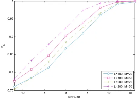
The detection probability is given by Fig. 6. First, we can see that increasing the static fading length L can enhance the accuracy of device detection, in the presence of unknown timing and channel fading. Taking a sample size M=200 for example, a rough gain of 5dB will be attained if L=50, compared to another case ofL=20. In contrast to a common sense, for a small static fading length (e.g.L=20), increasing the sample sizeM cannotalways achieve the detection gains, in the situation of asynchronous D2D device detection. As mentioned, only the improvement on the likelihood accuracy surpasses the enlargement of timing uncertainty, can the de-tection performance be improved, as the case of large static length L=50.
B. Uncorrelated timing drifts
[image:11.612.322.552.267.437.2]
-5 0 5 10 15
0.75 0.8 0.85 0.9 0.95 1
SNR /dB PD
[image:12.612.62.284.51.220.2]L=100, M=20 L=100, M=50 L=200, M=20 L=500, M=50
Fig. 6. Device detection performance in the context of correlated transmission intervals.
-10 -5 0 5 10 15 5
10 15 20 25 30 35 40 45 50 55
SNR /dB
M
S
E
of
t
im
ing dr
if
t
L=100, M=20 L=100, M=50 L=200, M=20 L=200, M=50
Fig. 7. MSE performance of dynamic timing drifts in the context of uncorrelated transmission intervals.
8.25 (samples) in high SNR regions (e.g. SNR>10dB). This is relatively different from the numerical results of correlated timing drifts. Meanwhile, we find that the estimation MSE of uncorrelated timing drifts will be higher than that of correlated drifts. Taking M=100 andL=50 for example, the mean MSE for uncorrelated drifts is about 8.22 samples when SNR=16dB, while the mean MSE under correlated drifts will only be 2.16 samples. This is mainly attributed to the underlying dynamics of correlated drifts, which may be further utilized to improve the estimation performance.
When it comes to varying fading channels, the estimation accuracy will be comparable to that of the correlated timing drifts. In the high SNR region, the slightly more accurate estimation will be obtained in the case of correlated timing drifts. Taking SNR=12dB for example, the MSE of uncorre-lated drifts is about 0.005 whenM=200 andL=50. While for the correlated drifts, the MSE becomes 0.0045.
The performance of device detection under uncorrelated timing drifts are shown by Fig. 9. Taking M=200 andL=50, when SNR is larger than 12dB, the right detection probability will be 1. We will see that, in this case, the residual errors of unknown timing drift is about 15 samples, while the relative
-10 -5 0 5 10 15 10-3
10-2 10-1 100 101
SNR /dB
M
S
E
of
c
hann
el
ga
in
[image:12.612.324.548.54.222.2]L=100, M=20 L=100, M=50 L=200, M=20 L=200, M=50
Fig. 8. MSE performance of time-dependent fading channels in the context of uncorrelated transmission intervals.
-10 -5 0 5 10 15 0.75
0.8 0.85 0.9 0.95 1
SNR /dB PD
L=100, M=20 L=100, M=50 L=200, M=20 L=200, M=50
Fig. 9. Device detection performance in the context of uncorrelated transmission intervals.
error of fading channels will be 0.005. By effectively sup-pressing the involved information uncertainties, the proposed scheme is applicable to asynchronous D2D device detection, even with varying fading gain and unknown timing drifts.
C. Comparative analysis
[image:12.612.62.288.267.432.2] [image:12.612.324.550.268.432.2]
-5 0 5 10 15
0.4 0.5 0.6 0.7 0.8 0.9 1
SNR /dB
PD Proposed: correlated Expectation: correlated, M/4 Expectation: correlated, 0 Proposed: uncorrelated Expectation: uncorrelated, M/4 Expectation: uncorrelated, 0
(a)
-2 0 2 4 6 8 10
2.9 3 3.1 3.2 3.3 3.4
Sensing SNR /dB
A
c
c
u
m
u
la
te
d
C
a
p
a
ci
ty (
b
it
s
/S
e
c
/H
z
)
Proposed scheme Expectation-based scheme
[image:13.612.83.527.55.234.2](b)
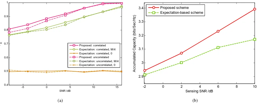
Fig. 10. (a) Device detection performance of the designed scheme vs the expectation likelihood-based methods. (b) The accumulated capacity for shared accessing scenario of different detection schemes.
can be available. In this case, the likelihood-based tech-nique can be utilized. To be specific, when the conditional likelihood p(zn|sn = 1,EM{Mn},EA{αn}) is larger than
p(zn|sn= 0), we will havesˆn=1, and otherwise,sˆn=0. Since
the timing driftsMn will be distributed in[−M/2, M/2], one
simple and direct solution is to assume EM{Mn} = 0. I.e.,
the detector will be totally unconscious of real-time drifts. From the simulation result, with the two-level information uncertainty aroused by varying fading and the timing drifts, the detection performance will be significantly deteriorated. For example, the right detection probability PD will be 0.5,
no matter what the SNR is. Similar results can be observed when the uncorrelated drifts are concerned.
In fact, more partial statistic information (i.e. expectation) on unknown timing drifts can be further exploited. For exam-ple, we note from simulation results that, when theexpectation
on timing deviations is configured to a half of the sample size (or maximum deviation), i.e.EM{Mn}=M/4, the detection
performance of likelihood-based methods will be improved, compared with the simple assumption EM{Mn} = 0. Even
so, the partial information inspired detection scheme still achieves the less attractive performance, as in Fig. 10-a. In comparison, by tracking two unknown LSI and suppressing the information uncertainty, a rough gain about 5∼6dB can be obtained by our new scheme.
Finally, we investigated the accumulated capacity in shared access scenarios. We consider two local links, one conducts primary transmissions and the other one (i.e. secondary link) manages to share the spectrum via a listen-before-talk strategy. Due to the false detection (with the probability p(H1|H0)),
the capacity of primary user will be degraded. The missed detection (with the probabilityp(H0|H1)), on the other hand,
will affect the shared capacity of secondary transmissions. Without losing generality, we assume the normalized capacity of primary user with no interference from shared transmission isCp, and the capacity when the missed detection occurs will
be decreased toCp0. The shared capacity of secondary user (i.e.
conducting proximity-based transmission) is Cs. It is easily
found the accumulated capacity is:
Ca=Cp·p(H1|H1)p(H1) +Cp0 ·[1−p(H1|H1)]p(H1)
+Cs·[1−P(H1|H0)]p(H0).
We then evaluated the promotion of accumulated capacity Ca by our proposed scheme. In numerical analysis, we
configured L = 20, M = 100, EM{Mn} = M/4,
p(H1)=p(H0)=0.5, Cp=2.32 bit/sec/Hz (i.e. SN RP=4),
Cp0=1.32 bit/sec/Hz (i.e. SIN RP=1.5), and Cs=4.39
bit/sec/Hz (i.e. SN RS=20). From Fig. 10-b, we noted the
proposed scheme can enhance the accumulated capacity Ca of shared accessing. Taking the sensing SNR of 10dB
for example, the accumulated capacity can be improved by 7% by using the new scheme, compared with a classical detection method (i.e. the likelihood-based detection utilizing the expectation of unknown LSI.)
More importantly, except for promoting the detection per-formance, the acquired LSI will be also of great significance, for example, to underlay D2D communications [48]. To be specific, the accurate fading gain will provide additional information for subsequent D2D mode selection and resource allocations. For example, consider two primary devices talk with each other via the time division duplexing (TDD) scheme, then the probed channel gain permits the real-time power adaption of shared transmission to limit its interference (e.g. with either peak or averaging interference constraint). As a result, the uninterrupted transmission of shared user and the harmonious coexistence between primary and secondary links would become a reality. To this end, the additional shared capacity can be also achieved, with the aid of our proposed scheme and the acquired channel information. Such additional benefits would be covered in our future studies.
V. CONCLUSIONS
fading channels. In order to achieve the reliable detection, we design a novel deep sensing paradigm to combat destructive effects from unknown LSI. The underlying dynamics of two unknown states are fully concerned, and a sequential Bayesian scheme is proposed, which acquires the varying timing drifts and fading channels when directly performing device detec-tion. To solve the complex MED problem, the two-stage recur-sive estimation is implemented, and the PF-based numerical approximation is further used to alleviate the computation complexity. Two types of timing drifts are considered, and the detection/estimation performance are numerically evaluated. It is demonstrated that, by dynamically tracking unknown drifts and fading gains, the detection performance will be improved significantly, compared to the expectation-based likelihood method. Our new scheme may further provide the useful information for transmission optimisation, e.g. the mode se-lection based on fading gains. By increasing the configuration flexibility, this scheme will be of promise to the emerging D2D communications, especially in adverse environments, e.g., out-of-coverage or publicity safety scenarios.
ACKNOWLEDGMENT
We greatly thank anonymous reviewers for their constructive comments and helpful feedback that allowed us to improve the paper significantly. We would also like to express our heartfelt thanks to Dr. Fahmy Suhaib of the University of Warwick, for his kind help in the hardware evaluation of the algorithm. This work was supported by Natural Science Foundation of China (NSFC) under Grant 61471061 and Grant 61571100.
REFERENCES
[1] X. Lin, J. G. Andrews, A. Ghosh, R Ratasuk, “An overview of 3GPP device-to-device proximity services,”IEEE Communications Magazine, vol. 52, no. 4, pp. 40-48, 2014.
[2] J. Seppala, T. Koskela, T. Chen, and S. Hakola, “Network controlled Device-to-Device (D2D) and cluster multicast concept for LTE and LTE-A networks,” in Proc. ofIEEE Wireless Communications and Networking Conference (WCNC), pp. 986-991, March 2011.
[3] M. J. Yang, S. Y. Lim, H. J. Park, and N. H. Park, “Solving the data overload: Device-to-device bearer control architecture for cellular data offloading,”IEEE Vehicular Technology Magazine, vol. 8, no. 1, pp. 31-39, 2013.
[4] L. Lei, Y. Kuang, X. (Sherman) Shen, C. Lin, and Z. Zhong, “Resource Control in Network Assisted Device-to-Device Communications: Solu-tions and Challenges,”IEEE Communication Magazine, vol. 52, no. 6, pp. 108-117, Jun. 2014.
[5] Cisco Visual Networking Index, Global Mobile Da-ta Traffic Forecast Update 2012-2017, White Paper, http//www.cisco.com/en/US/solutions/collateral/ns341/ns525/ns537/ns705/ ns827/ whitepaperc11-520862.html, 6th, 2013 Feb.
[6] X. M. Shen, “Device-to-device communication in 5G cellular networks,” IEEE Network, vol. 29, no. 2, pp.2-3, 2015.
[7] C. Q. Fan, B. Li, C. L. Zhao, W. S. Guo, Y.-C. Liang, “Learning-based Spectrum Sharing and Spatial Reuse in mm-Wave Ultra Dense Networks,” IEEE Transactions on Vehicular Technology, 2017, DOI: 10.1109/TVT.2017.2750801.
[8] Y. Peng, Q. Gao, S. Sun, and Y. Zheng, “Discovery of device-device prox-imity: Physical layer design for D2D discovery,” in Proc. ofIEEE/CIC International Conference on Communications in China-Workshops (CI-C/ICCC), pp. 176-181, 2013.
[9] A. Asadi, Q. Wang, V. Mancuso, “A survey on device-to-device communi-cation in cellular networks,”IEEE Communications Surveys&Tutorials, vol. 16, no. 4, pp.1801-1819, 2014.
[10] G. Fodor, E. Dahlman, G. Mildh, “Design aspects of network assisted device-to-device communications,”IEEE Communications Magazine, vol. 50, no. 3, pp.170-177, 2012.
[11] E. Yaacoub, O, Kubbar, “Energy-efficient device-to-device commu-nications in LTE public safety networks,” in Proc. of IEEE Global Communications Conference (Globecom Workshops), pp.391-395, 2012. [12] G. Fodor, S. Parkvall, S. Sorrentino, et.al. “Device-to-device commu-nications for national security and public safety,” IEEE Access, vol. 2, pp.1510-1520, 2014.
[13] B. Kaufman, J. Lilleberg, and B. Aazhang. “Spectrum Sharing Scheme Between Cellular Users and Ad-hoc Device-to-Device Users,” IEEE Transactions on Wireless Communications, vol. 12, no. 3, pp. 1038-1049, March 2013.
[14] C. Xu, L. Song, Z. Han, Q. Zhao, X. Wang, and B. Jiao, “Interference-aware resource allocation for device-to-device communications as an underlay using sequential second price auction,” in Proc. of IEEE International Conference on Communications (ICC), pp. 445-449, June 2012.
[15] J. Ma, G. Y. Li, and B. H. Juang, “Signal Processing in Cognitive Radio,” The Proceedings of IEEE, vol. 97, no. 5, May 2009, pp. 805-823. [16] E. Axell, G. Leus, E. G. Larsson, and H. V. Poor, “Spectrum Sensing
for Cognitive Radio: State-of-the-art and recent advances,”IEEE Signal Processing Magazine, vol. 29, no. 3, May 2012, pp. 101-116.
[17] H. Tang, Z. Ding, B. C. Levy, “Enabling D2D communications through neighbor discovery in LTE cellular networks,” IEEE Transactions on Signal Processing, vol. 62, no. 19, pp. 5157-5170, October 2014. [18] 3GPP “3rd generation partnership project technical specification group
SA study on architecture enhancements to support proximity services (ProSe) (Release12),” TR#23.703#V0.4.1, June 2013.
[19] N. Wang and T. A. Gulliver, “Low-Complexity Census-Based Collabora-tive Compressed Spectrum Sensing for CogniCollabora-tive D2D Communications,” in Proc. of 2015 IEEE Global Communications Conference (GLOBE-COM), 6-10th Dec. 2015, pp. 1-7.
[20] Y.-C. Liang, K. C. Chen, G. Y. Li, and P. M¨ah¨onen, “Cognitive radio networking and communications: an overview,” IEEE Transactions on Vehicular Technology,vol. 60, no. 7, September 2014, pp. 3386-3407. [21] F. F. Digham, M. S. Alouini, and M. K. Simon, “On the Energy
Detection of Unknown Signals Over Fading Channels,” in Proc. ofIEEE international Conference on Communications (ICC), Anchorage, AK, May 2003, vol. 5, pp. 3575-3579.
[22] Y. H. Zeng, Y. C. Liang, “Eigenvalue-based Spectrum Sensing Algo-rithms for Cognitive Radio,”IEEE Trans Commun., vol. 57, 2009, pp. 1784-1793.
[23] B. Li, C. L. Zhao, M. W. Sun, Z. Zhou, A. Nallanathan, “Spectrum Sensing for Cognitive Radios in Time-Variant Flat Fading Channels: A Joint Estimation Approach,”IEEE Transactions on Communications, 2014, vol. 62, no. 8, pp. 2665-2680.
[24] B. Li, M. W. Sun, X. F. Li, A. Nallanathan, C. L. Zhao, “Energy Detection based Spectrum Sensing for Cognitive Radios Over Time-Frequency Doubly Selective Fading Channels,” IEEE Transactions on Signal Processing,vol. 63, no. 2, Jan. 2015, pp. 402-417.
[25] B. Li, S. H. Li, A. Nallanathan, C. L. Zhao, “Deep Sensing for Future Spectrum and Location Awareness 5G Communications,”IEEE Journal Selected Areas Communications, vol. 33, no. 7, 2015, pp. 1331-1344. [26] B. Ristic and A. Farina, “Target tracking via multi-static Doppler shifts,”
IET Proc. Radar, Sonar Navig., vol. 7, no. 5, 2013, pp. 508-516. [27] B.-T. Vo, D. Clark, B.-N. Vo, and B. Ristic, “Bernoulli
forward-backward smoothing for joint detection and tracking,”IEEE Trans. Signal Processing, vol. 59, No. 9, 2011, pp. 4473-4477.
[28] S. Tekinalpl, A. A. Alatan, “Efficient Bayesian Track-Before-Detect,” in Proc. of 2006 International Conference on Image Processing (ICIP), 2006, pp. 2793-2796.
[29] R. Mahler,Statistical Multisource Multitarget Information Fusion. Nor-wood, MA, USA: Artech House, 2007.
[30] B.-T. Vo and B.-N. Vo, “A Random Finite Set Conjugate Prior and Application to Multi-target Tracking,” in Proc.7th IEEE Int. Conf. Intell. Sens., Sens. Netw. Inf. Proc. (ISSNIP), Adelaide, Australia, Dec. 2011, pp. 431-436.
[31] M. Jung, K. Hwang, and S. Choi, “Joint mode selection and power allocation scheme for power-efficient device-to-device (D2D) communi-cation,” in Proc. ofIEEE Vehicular Technology Conference (VTC-Spring), pp. 1-5, 2012.
[32] J. Seppala , T. Koskela , T. Chen and S. Hakola, “Network controlled Device-to-Device (D2D) and cluster multicast concept for LTE and LTE-A networks,” in Proc. ofIEEE Wireless Communications&Networking Conference (WCNC), pp. 986-991, 2011.
[34] B. Li, S. H. Li, Y. J. Nan, A. Nallanathan, C. L. Zhao, Z. Zhou “Deep Sensing for Next-generation Dynamic Spectrum Sharing: More Than Detecting the Occupancy State of Primary Spectrum,”IEEE Transactions on Communications,vol. 63, no. 7, 2015, pp. 2442-2457.
[35] P. Sadeghi, R. Kennedy, P. Rapajic, R. Shams, “Finite-state Markov Modeling of Fading Channels: A Survey of Principles and Applications,” IEEE Signal Processing Magazine, vol. 25, no. 5, 2008, pp. 57-80. [36] H. S. Wang, N. Moayeri, “Finite-state Markov Channel: A Useful Model
for Radio Communication Channels,”IEEE Transactions on Vehicular Technology,vol. 44, no. 1, Feb. 1995, pp. 163-171.
[37] H. S. Wang, P. Chang, “On Verifying the First Order Markovian Assumption for A Rayleigh Fading Channel Model,”IEEE Transactions on Vehicular Technology,vol. 45, no. 2, May 1996, pp. 353-357. [38] W. B. Davenport Jr. and W. L. Root,An Introduction to the Theory of
Random Signals and Noise,New York : IEEE Press, 1958.
[39] S. J. Miller, M. J. Nigrini. “The modulo 1 central limit theorem and Benford’s law for products,”arXiv preprint math/0607686,2006. [40] P. Pedrosa, R. Dinis, F. Nunes, et al. “Phase Drift Estimation and Symbol
Detection in Digital Communications: A Stochastic Recursive Filtering Approach,”IEEE Communications Letters,2012, vol. 16, no. 16, pp.854-857.
[41] B.-T. Vo, B.-N. Vo, and A. Cantoni, “Bayesian filtering with random finite set observations,”IEEE Trans. Signal Process., vol. 56, no. 4, pp. 1313-1326, 2008.
[42] B. Ristic, Ba-Tuong Vo, Ba-Ngu Vo, A. Farina, “A Tutorial on Bernoulli Filters: Theory, Implementation and Applications,”IEEE Trans. Signal Process., vol. 61, no. 13, July, 2013, pp. 3406-3430.
[43] Z. Chen, “Bayesian Filtering: From Kalman Filters to Particle Filters, and Beyond,”Statistics, 2003.
[44] P. M. Djuric, J. H. Kotecha, J. Q Zhang, Y. F. Huang, T. Ghirmai, M. F. Bugallo, J. Miguez, “Particle filtering,”IEEE Signal Processing Magazine, vol. 20, no. 5, 2003, pp. 19-38.
[45] A. Doucet, S. Godsill, C. Andrieu, “On sequential Monte Carlo sampling methods for Bayesian filtering,”Statistics and computing, 2000, vol. 10, no. 3, pp. 197-208.
[46] Y. C. Liang, Y. H. Zeng, E. C. Y. Peh et al. “Sensing-Throughput Tradeoff for Cognitive Radio Networks,”IEEE Transactions on Wireless Communications,vol. 7, no. 4, 2008, pp. 1326-1337.
[47] L. Deng, C. Chakrabarti, N. Pitsianis, et al. “Automated optimization of look-up table implementation for function evaluation on FPGAs,” in Proc of SPIE, 2015, 7444, pp. 744413-744413-9.