On the error in phase transition computations for compressed sensing

warwick.ac.uk/lib-publications

Manuscript version: Author’s Accepted Manuscript

The version presented in WRAP is the author’s accepted manuscript and may differ from the

published version or Version of Record.

Persistent WRAP URL:

http://wrap.warwick.ac.uk/117761

How to cite:

Please refer to published version for the most recent bibliographic citation information.

If a published version is known of, the repository item page linked to above, will contain

details on accessing it.

Copyright and reuse:

The Warwick Research Archive Portal (WRAP) makes this work by researchers of the

University of Warwick available open access under the following conditions.

Copyright © and all moral rights to the version of the paper presented here belong to the

individual author(s) and/or other copyright owners. To the extent reasonable and

practicable the material made available in WRAP has been checked for eligibility before

being made available.

Copies of full items can be used for personal research or study, educational, or not-for-profit

purposes without prior permission or charge. Provided that the authors, title and full

bibliographic details are credited, a hyperlink and/or URL is given for the original metadata

page and the content is not changed in any way.

Publisher’s statement:

Please refer to the repository item page, publisher’s statement section, for further

information.

On the Error in Phase Transition Computations for

Compressed Sensing

Sajad Daei, Farzan Haddadi, Arash Amini, Martin Lotz

Abstract—Evaluating the statistical dimension is a common tool to determine the asymptotic phase transition in compressed sensing problems with Gaussian ensemble. Unfortunately, the exact evaluation of the statistical dimension is very difficult and it has become standard to replace it with an upper-bound. To ensure that this technique is suitable, [1] has introduced an upper-bound on the gap between the statistical dimension and its approximation. In this work, we first show that the error bound in [1] in some low-dimensional models such as total variation and `1 analysis minimization becomes poorly large. Next, we develop a new error bound which significantly improves the estimation gap compared to [1]. In particular, unlike the bound in [1] that fails in some settings with overcomplete dictionaries, our bound exhibits a decaying behavior in such cases.

Index Terms—statistical dimension, error estimate, low-complexity models.

I. INTRODUCTION

U

NDERSTANDING the behavior of random compressed sensing problems in transition from absolute failure to success (known as phase transition) has been the subject of research in recent years [1]–[8]. Most of these works concentrate on simple sparse models and do not allude to the challenges in other dimensional structures such as low-rank matrices, block-sparse vectors, gradient-sparse vectors and cosparse (also known as analysis sparse [9]) vectors. For simplicity, we associate such structures with their common recovery techniques and rename the structures accordingly. For instance, total variation (TV), `1 analysis and `1,2 minimiza-tion refer to both the recovery techniques and the underlying low-dimensional structures. In this work, we revisit linear inverse problems with the aim of recovering a vector xPRn

from a few random linear measurements y“AxPRm. This

is summarized as solving the following convex program:

Pf : min

zPRn

fpzq

s.t. y“Az, (1)

where, APRmˆn is the measurement matrix whose entries

are i.i.d. random variables with normal distribution and f is a convex penalty function that promotes the low-dimensional structure. A major subject of recent research is the number of Gaussian measurements (the number of rows inA) one needs to recover a structured vectorxfromyPRm. In [3], a bound

is obtained using polytope angle calculations with asymptotic sharpness in case off “ } ¨ }1. A link between the number of

S. Daei and F. Haddadi are with the School of Electrical Engineering, Iran University of Science & Technology. A. Amini is with EE department, Sharif University of Technology. M. Lotz is with the Mathematics Institute, University of Warwick.

required measurements and the error in the denoising problem is investigated in [8]. For the particular case off “ } ¨ }TV in

Pf, we need to consider the denoising problem

p

x“arg min

zPRn

τ σ}z}TV` 1

2}y´z} 2

2, (2)

where y “ x`w with w being an additive noise drawn fromNp0, σ2_I

q. If we define the worst-case normalized mean squared error (NMSE) as

NMSE:“ lim

σÑ0τěinf0

E}x´x_p}2₂

σ2 , (3)

then, the result in [8] implies that the value of NMSE is a sharp estimate of the required number of measurements (for PTV) in the asymptotic case. Also, in [7], the authors showed that the mentioned NMSE is the same as the number of required measurements that TV approximate message passing (TV-AMP) algorithm needs. [2] introduced a general framework for obtaining the number of Gaussian measurements in different low-dimensional structures using Gordon min-max inequality [10] and the concept of atomic norms. Specifically, it was shown thatω2_pDpf,x

q XBnq `1measurements are sufficient. Here, Dpf,xq is the descent cone of f at x P Rn and ω2_pDpf,x

q XBnq is the squared Gaussian width, which intuitively measures the size of this cone. In [1], it has been shown that the statistical dimension of this cone, which is defined below and differs from the squared Gaussian width above by at most 1, specifies the phase transition of the [random] convex programPf from absolute failure to absolute success:

δpDpf,xqq:“Edist2pg,conepBfpxqqq. (4)

δpDpf,xqq is the average distance of a standard Gaussian i.i.d. vector g P Rn from non-negative scalings of the

sub-differential at point x P Rn. So far, we know that a phase

transition exists inPf and its boundary is interpreted via the statistical dimension. A natural question is how we can find an expression for the phase transition curve. The upper-bound forδpDpf,xqq, first used in the context of`1minimization by Stojnic ( [6]), is given by:

δpDpf,xqq ďinf

tě0E dist 2

pg, tBfpxqq:“Uδ. (5)

However, it is still unknown whetherUδ is sharp for different

low-dimensional structures. For ease of notation, we define the errorEδ by:

Here,Uδ represents a sufficient number of measurements that Pf needs for successful recovery. In [1], implicit formulas

are derived for the upper-bound (5) in case of`1 and nuclear norm. Recently, an explicit upper-bound for Uδ in case of

`1 analysis and TV minimization is presented in [11]. The proposed bound depends on a notion called “generalized analysis sparsity” and is numerically observed to be tight for many analysis operators. In [1], a general upper-bound expression for Eδ (known as the error estimate) for various

structure-inducing functions (e.g.`1) is proposed (see Theorem 1). For the cases of `1 and nuclear norm minimization, it is further shown that the normalized error estimate Epp

n (and thus Eδ

n ) vanishes in high dimensions. This result confirms thatUδ

is a good surrogate for δpDpf,xqq. However, the asymptotic behavior of Eδ

n in cases of}¨}1,2,}Ω¨}1and}¨}TV :“ }Ωd¨}1

where

Ωd“

»

— — — –

1 ´1 0 ¨ ¨ ¨ 0 0 1 ´1 ¨ ¨ ¨ 0

. ._. . ._. . ._. 0 ¨ ¨ ¨ ¨ ¨ ¨ 1 ´1

fi

ffi ffi ffi fl

PRn´1ˆn, (7)

is not studied. Thus, one could simply think of the following problems:

1) DoesUδ provide a fair estimate of the statistical

dimen-sion?

2) How to quantify the gap between the exact phase transi-tion curve and the one obtained viaUδ?

3) Can one extend the previous error bounds obtained for`1 minimization in [1] to other low-dimensional structures such as block sparsity, TV and `1 analysis?

In this work, we try to find answers to these ques-tions. Specifically, we want to study how well Uδ describes

δpDpf,xqqin low-dimensional structures represented by} ¨ }1, }¨}1,2,}¨}˚,}Ω¨}1and}¨}TV:“ }Ωd¨}1. A genericΩPRpˆn

can be tall, i.e.pąn, or fat, i.e.pďn; due to the similarity of the arguments used in this paper, we include square matrices in the category of fat matrices. TallΩ matrices cover various redundant1 _{analysis operators that are common in practice;}

in particular, redundant wavelet frames [12], and redundant random frames (widely used as a benchmark template in [9], [11], [13], [14]). Also fat matrices include examples such as the one-dimensional finite difference operator Ωd and

non-redundant random analysis operators (used in [11, Section 3.3]). We call a signalxPRn an analysis-sparse vector (also

called as cosparse vector [9]) with respect to the analysis operator Ω P Rpˆn if after applying Ω the resulting vector

becomes sparse; i.e., Ωxis sparse. We denote the support set of Ωx with S; similarly, S stands for the zero set of Ωx. The number of zeros in Ωx, i.e.,|S|, is called the cosparsity of x with respect to Ω [9], [11], [14]. We should highlight that in most of the existing literature regarding the`1-analysis problem it is assumed that Ω P Rpˆn has rows in general

position2_.

1_{The term redundant refers to an analysis operator with more number of}

rows than columns.

2_{Every subset ofnrows ofΩare linearly independent.}

Uδ δpDp} ¨ }1,xqq Eδ

n p Ep

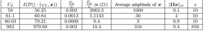
[image:3.612.80.299.255.309.2]

n in (21) s 9.458 9.0905 0.0003 0.064 1 16.828 16.8 0.0003 0.045 2 23.4544 23.04 .0005 0.036 3 61.244 60.84 0.0004 0.02 10 104.1814 104.04 0.0001 0.015 20

Table I: In this table, we examine the error estimate [1] for functionf“ } ¨ }1

and signalxwith dimensionn“1000. The upper-boundUδ is computed using the package SNOW in [1]. The true sample complexity is denoted by δpDp}¨}1,xqqand computed by squaringωpDp}¨}1,xqXBnq(see Appendix E for more details). For the considered class ofxsignals, we observe that there is a negligible gap between Epp

n in [1] and the true normalized error Eδ

n.

A. Motivation

Tables I and II present the results of a computer experiment designed to evaluate the error ofUδ in estimating the statistical

dimension. In two experiments shown in Tables I and II, we test the error bound for`1and TV minimization. The value of

δpDpf,xqqwhich is approximately equal toω2_pDpf,x qXBnq, is computed using the procedure proposed in [11, Section B.2] (see Appendix E). In the first experiment, for each sparsity level, we construct a sparse vector x P R1000 with random

non-zero values (distributed as Np0,?1000q) at uniformly random locations. In the second experiment, we setΩ“Ωd,

and generate a gradient sparse vector x PR1000 as the sum

of two components: a small but non-zero component in the spacenullpΩ_Sq, and a large component in the spacenullpΩq. The notationΩ_S refers to the matrixΩ restricted to the rows indexed byS (see Section IV-A for more details). For Tables I and II, the upper-bound (5) is obtained by [1, Equation D.6] and numerical optimization3, respectively. As shown in Tables I and II, there exists a gap between the true errorEδ and the

state of the art theoretical error estimate Epp in (21). While

the normalized gap, i.e., |Eδ´Epp|

n is negligible in the `1 case

(Table I), it is considerable in case of TV minimization (Table II). Now, a natural question that arises is: can we find a better bound that reduces the gap?

B. Contributions

In this work, we rigorously analyze the error of estimating the phase transition. The significance of this error is to have a good understanding about the required number of measure-ments thatPfneeds to recover a structured vector from

under-sampled measurements. Our analysis is general and holds for a variety of low-dimensional structures including sparse, block-sparse, analysis sparse and gradient-sparse vectors, as well as low-rank matrices. In brief, the contributions of this work can be listed as follows.

1) Identifying a failure regime for [1]: Forf “ }Ω¨ }1 in

Pf, the error estimate of [1] shown in (21), can become

remarkably large for some specific signals and analysis operators. For fat analysis operators, a typical signal x

with such property is constructed as:

x“PnullpΩSqw`PnullpΩqcPR

n_{, (8)}

3_{See also [15, Section 4] which proposes a numerical method to calculate}

Uδ δpDp} ¨ }TV,xqq Enδ p Ep

n in (21) Average amplitude ofx }Ωx}8 s

58 56.25 0.002 2063.3 1000 0.1 10

61.1 60.84 0.0013 5.1143 30 4 10

80.03 79.21 0.0008 0.4 3 0.9 10

[image:4.612.132.478.53.106.2]

982 979.69 0.002 10.4 316 0.4 850

Table II: In this table, we examine the TV error bound for gradient sparse signals with dimensionn“1000. The upper-boundUδ is obtained by Monte Carlo simulations and numerical optimization. The true sample complexityδpDp} ¨ }TV,xqq «ω2pDp} ¨ }TV,xq XBnqis obtained using the approach presented in Appendix E. The large values of Epp

n observed in this table are not necessarily caused by approximatingδpDpf,xqqwithUδ.

where w,cP Rn are arbitrary vectors. For tall analysis

operators, we can find pairs of Ω andx for which the error estimate [1] explodes. We precisely investigate this in Section IV.

2) Obtaining an error bound forδpDpf,xqqwith rather gen-eral fp¨q: δpDpf,xqqprecisely determines the boundary of failure and success ofPf. However, exact computation

of δpDpf,xqqis very difficult. It is common to approxi-mate δpDpf,xqqwithUδ. By providing an error bound,

we formally show that this approximation is good. More precisely, we show that

Eδ

n ďh2pβ, ωq, (9)

where β depends on Bfpxq, and h2pβ, ωq is a function ofβ andωpDpf,xq XBnqthat is succinctly shown byω. Under certain conditions, we show thath2pβ, ωqvanishes asngrows sufficiently large. To a great extent, the setting considered forf (see (30)) is nonrestrictive. In particular, it includes the important special cases of}Ω¨ }1 for tall and fat analysis operators.

In contrast to the error estimate of [1] that directly depends on xPRn, our bound is determined byBfpxq. Besides, our error bound holds even for rank-deficient fat Ω P Rpˆn matrices. We should emphasize that our

error estimate bound is not sharp in all cases of analysis operators and does not necessarily fill the gap between

Eδ andEpp in (21). In fact, there are various settings in

which the bound in [1], our bound, or both are effective.

C. Notation

Throughout the paper, scalars are denoted by lowercase letters, vectors by lowercase boldface letters, and matrices by uppercase boldface letters. The ith element of the vector x

is given either by xpiq or xi. The notation p¨q: stands for

the pseudo-inverse operator. We reserve calligraphic uppercase letters for sets (e.g. S) and denote the cardinality of a set S by |S|. The complement of a set S in t1, ..., nu (briefly represented asrns) is denoted byS. Similarly, the complement of an eventE is shown byE. For a matrixX PRmˆn and a

subset S Ď rns, the notation XS refers to the sub-matrix of X by including the rows indexed byS. Similarly, forxPRn, xS stands for the vector inRn that coincides withxat entries

indexed by S and zero elsewhere. Also, we use the notation

r

xS to represent a sub-vector ofx inR|S|, that is formed by

discarding the zero entries not indexed in S. The null-space of linear operators is denoted bynullp¨q. For a matrixΩ, the

operator norm is defined as }Ω}pÑq “ sup }x}pď1

}Ωx}q. Also,

κpΩq :“ σmaxpΩq

σminpΩq denotes the condition number of Ω. The

polar K˝ _{of a cone K Ă}

Rn is the set of vectors forming

non-acute angles with every vector inK, i.e.

K˝_{“ tvP}

Rn:xv,zy ď0 @zPKu. (10)

Bn _and

Sn´1 stand for the unit ball txP Rn : }x}2 ď1u and unit sphere tx P Rn : }x}2 “ 1u, respectively. PC is the matrix associated with the orthogonal projection onto the subspace C, that maps a vector inRn onto the subspace

CĂRn.

D. Outline

The paper is organized as follows. The required concepts from convex geometry are reviewed in Section II. Section III discusses two approaches in obtaining the error estimate. Section V is dedicated to present our main contributions. In Section IV, we investigate the estimate in [1] and introduce some examples for which the error estimate does not work. In Section VI, numerical experiments are presented which confirm our theory. Finally, the paper is concluded in Section VII.

II. CONVEXGEOMETRY

In this section, a review of basic concepts of convex geometry is provided.

A. Descent Cones

The descent coneDpf,xqat a pointxPRnconsists of the

set of directions that do not increasef and is given by:

Dpf,xq “ď

tě0

tzPRn:fpx`tzq ďfpxqu. (11)

The descent cone reveals the local behavior of f near xand is a convex set. There is also a relation between decent cone and subdifferential [16, Chapter 23] given by:

D˝

pf,xq “conepBfpxqq:“ ď

tě0

tBfpxq. (12)

B. Statistical Dimension

Definition 1. Statistical Dimension [1]: Let C Ď Rn be a

closed convex cone. The statistical dimension ofC is defined as:

δpCq:“E}PCpgq}22“Edist 2

pg,C˝

wherePCpxqis the projection ofxPRnonto the setCdefined

as:PCpxq “arg min zPC

}z´x}2.

The statistical dimension extends the concept of linear subspaces to convex cones. Intuitively, it measures the size of a cone. Furthermore,δpDpf,xqqdetermines the precise location of transition from failure to success in Pf.

C. Gaussian width

Definition 2. The Gaussian width of a setC is defined as:

ωpCq:“Esup

yPC

xy,gy. (14)

The relation between statistical dimension and Gaussian width is summarized in the following [2, Proposition 3.6], [1, Proposition 10.2].

ωpCXSn´1q ďωpCXBnq “_E}PCpgq}2“E distpg, C˝q, (15)

ω2pCXBnq “ pE}PCpgq}2q2ďδpCq. (16)

It is shown in [1, Proposition 10.2]. that the quantitiesω2 pCX

BnqandδpCqdiffer numerically by at most1.

D. Optimality Condition

In the following, we characterize when Pf succeeds in the noise-free case.

Proposition 1. [2, Proposition 2.1] Optimality condition: Let

f be a proper convex function. The vectorxPRnis the unique optimal point of Pf if and only ifDpf,xq XnullpAq “ t0u.

The next theorem determines the number of measurements needed for successful recovery of Pf for any proper convex

functionf.

Theorem 1. [1, Theorem 2]: Letf :_Rn

ÑRY t˘8u be a proper convex function and xPRn a fixed vector. Suppose that m independent Gaussian linear measurements of x are observed via y“AxPRm. If

měδpDpf,xqq ` c

8 logp4

ηqn, (17)

for a given probability of failure (tolerance) η P r0,1s, then, we have

PpDpf,xq XnullpAq “ t0uq ě1´η. (18)

Besides, if

mďδpDpf,xqq ´ c

8 logp4

ηqn, (19)

then,

PpDpf,xq XnullpAq “ t0uq ďη. (20)

III. RELATEDWORKS INERRORESTIMATION

For bounding the distance betweenδpDpf,xqqandUδ, two

different approaches are proposed in [1], [17]. In the following, we briefly describe these methods.

Result 1. [1, Theorem 4.3] Let f be a norm. Then, for any

xPRnzt0u:

0ďEδ ď

NumE

hkkkkkkikkkkkkj 2 sup

sPBfpxq

}s}2

f´ x

}x}2

¯ :“Epp. (21)

Result 2. [17, Proposition 1] Suppose that for xPRnzt0u,

Bfpxqsatisfies a weak decomposability assumption:

Dz0P Bfpxqs.t.xz´z0,z0y “0, @zP Bfpxq. (22)

Then4_,

inf

tě0Edistpg, tBfpxqq ďωpDpf,xq XB

n

q `6. (23)

A. Explanations

Result 2 presents an error estimate for the Gaussian width of the descent cone (restricted to the unit ball) that is used to upper-bound the number of Gaussian measurements in various low-dimensional structures [2, Section 3.1]. For functionsf “ } ¨ }1, } ¨ }1,2 and } ¨ }˚, the constraint (22) is satisfied (see

Section V-A). Forf “ }Ω¨ }1, however, this constraint is not generally guaranteed (see Appendix F).

Unlike Result 2, the error estimate (21) depends on Bf at the ground-truth vector x, and the vector x itself. Although [1, Theorem 4.3] restrictsf to be a norm, the provided proof remains valid for semi-norms such as TV. The error bound in (21), is effective for many structure-inducing functions including `1,`1,2, and nuclear norm. Particularly,

p

Ep

n

asymp-totically vanishes in these cases. However, the normalized error estimate Epp

n is large in some cases of `1 analysis and

TV minimization and does not reflect the actual error Eδ

n; in

Section IV-A, we study some examples. A naive interpretation of this fact is thatUδ is a poor approximation of δpDpf,xqq

in those cases. Fortunately, as we show in Section V, this argument is invalid, which in turn suggests that (21) is a loose bound in those cases.

IV. THE STUDY OF EXISTING RESULTS

A. Result 1 for various low-complexity models

Before we describe our contributions in Section V, we first evaluate the error estimate (21) when f is any of `1, `1,2,

nuclear norm, or `1-analysis for different analysis operators. An important observation is that the error estimate (21) is increasing with }x}2

fpxq; thus, whenever this term becomes large,

we might obtain a loose upper-bound. To better clarify this point, we study the case of `1-analysis in three categories of fat analysis operatorsΩ, rank-deficient tall analysis operators

Ω, and full-rank tall analysis operatorsΩ.

4_{This result is wrongly interpreted as inf}

tě0 b

Edist2pg, tBfpxqq ď

‚ Sparse vectors

Since δ`Dp} ¨ }1,xq ˘

“δ`Dp} ¨ }1,sgnpxqq ˘

, the bound

p

Ep in (21) can be written in terms ofsgnpxq:

p

Ep“

2 sup_}z

S}8ď1}sgnpxq `zS}2 }sgnpxq}1

}sgnpxq}2

ě2}sgnpx?q `1S}2

s “

2?n

?

s , (24)

where the inequality is for choosing a point 1_S in the feasible set}z_S}8 ď1. The above expression may lead

to large errors in low sparsity regimes (s!n), however, limnÑ8

p

Ep

n “0. This shows thatUδ is asymptotically a

fair approximation ofδ`Dp} ¨ }1,xq ˘

.

‚ Block-sparse Vectors

With the same approach as in the previous case, the actual error estimate is lower-bounded by

p

Epě

2?q

?

s (25)

where sand qstand for the number of non-zero blocks and the total number of blocks respectively. Again for small s, the error can become large whilelimqÑ8

p

Ep

q “

0; thus, Uδ is asymptotically a fair approximation of

δ`Dp} ¨ }1,2,xq ˘

.

‚ Low-rank Matrices

Let X P Rn1ˆn2 _{be the rank r ground-truth}

ma-trix (n1 ě n2) with the SVD decomposition X “

Un1ˆn1Σn1ˆn2V

H

n2ˆn2 (alternatively, we have the

re-duced SVD decomposition as X “Un1ˆrΣrˆrV

H n2ˆr).

Since δ`Dp} ¨ }˚,Xq

˘

“δ`Dp} ¨ }˚,Un1ˆrV

H n2ˆrq

˘ , we can replace X withUn1ˆrV

H

n2ˆrin (21):

p

Ep“

2 sup_}P

TKpZq}2Ñ2ď1}Un1ˆrV

H

n2ˆr`PTKpZq}F

}Un1ˆrVnH2ˆr}˚ }Un1ˆrVnH2ˆr}F

,

(26)

where

PTKpZq “

´

I´PspanpUn₁ˆrq

¯

Z

´

I´PspanpVn₂ˆrq

¯

.

Now, by setting

Z“Un1ˆn2

„

0 0

0 In2´r



V_nH 2ˆn2

in (26), we obtain a lower-bound onEpp as

p

Epě

2}Un1ˆn2V

H n2ˆn2}F

}Un1ˆrVnH2ˆr}˚ }Un1ˆrVnH2ˆr}F

“ 2 ?

n2 ?

r . (27)

Similar to the previous cases, when r! n2, the bound becomes large, while,limn1,n2Ñ8

p

Ep

n1n2 “0. This shows

that Uδ is asymptotically a fair approximation ofδ

` Dp} ¨ }˚,xq

˘ .

‚ Cosparse vectors (fat analysis operators)

For fat Ω P Rpˆn, the nullpΩq is non-trivial, and we can choose c such that PnullpΩqc ‰ 0. Now, if x “

PnullpΩ_Sqw`PnullpΩqc, wherew is an arbitrary vector,

the denominator of the bound in (21) can be written as

}Ωx}1 }x}2

“ }ΩSPnullpΩSqw}1 }PnullpΩ_Sqw`PnullpΩqc}2

. (28)

By increasing the norm of c using a scalar multiplier, the above fraction decreases. In other words, we can make the denominator of the error bound (21) arbitrarily small (alternatively enlarge the error bound (21)). One of the well-known examples in this category is the finite difference operator Ωd, where nullpΩdq consists

of constant vectors. For this example, the denominator can be reduced by setting c “ α1nˆ1 P nullpΩdq and

α"1.

‚ Cosparse vectors (rank-deficient tall analysis

opera-tors)

Similar to the previous case,nullpΩqis non-trivial. Thus, the same approach can be devised to make the bound in (21) arbitrarily large.

‚ Cosparse vectors (full-rank tall analysis operators)

WhenΩis a full-rank and tall matrix, we cannot gener-ally find xthat results in a small value of }Ωx}1

}x}2 . Here,

we show the existence of pairs pΩ,xq for which the aforementioned ratio becomes arbitrarily small.

Let|S| ąn,|S| ăn,σą0and define

A_|S|ˆn “U|S|ˆndiagt1,1, . . . ,1

loooomoooon

pn´1qtimes

, σuV_nˆnT ,

where U_|S|ˆn and Vnˆn are arbitrary incomplete and

complete unitary matrices, respectively. It is evident that

A_|S|ˆn is a full-rank tall matrix. Let ui and vj stand

for the ith and jth columns of U and V, respectively. We know that A vn “ σun. Now, define B_|S|ˆn “

rv1, . . . ,v_|S|sT (since |S| ă n, this is possible). Obvi-ously,B vn“0. Finally, we define

Ω“ „

A B



, x“vn, S“ t1, . . . ,|S|u,

S“ t|S| `1, . . . ,|S| ` |S|u.

Indeed, the design is such thatΩS “Aand ΩS “B. AsAhas full column rank,Ωis also a full-rank matrix. It is straightforward to check thatxPnullpΩ_Sq, and

}Ωx}1 }x}2

“ }Ωx}1“ › › › › „ A B  vn › › › › 1

“ }Avn}1“σ}un}1.

Now, we can reduceσwhile keeping the rest untouched. In this way, we construct non-trivial pairs of pΩ,xqfor which the ratio }Ωx}1

}x}2 can be set arbitrarily small.

Remark 1. The value of Epp provides an upper-bound on

the gap betweenUδ andδ

`

Dpf,xq˘. However, its normalized

value (e.g., Epp

n in the `1 minimization) is important in

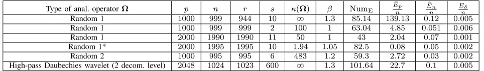
Type of anal. operatorΩ p n r s κpΩq β NumE p Ep

n p En

n Eδ

n Random 1 1000 999 944 10 8 1.3 85.14 139.13 0.12 0.005

Random 1 1000 999 999 2 100 1 63.04 4.85 0.051 0.006

Random 1 2000 1990 1990 11 50 1 43 2.04 0.07 0.001

Random 1* 2000 1995 1995 10 1.94 1.05 82.5 0.08 0.05 0.002

Random 2 1000 995 995 6 483 1.2 59.3 2.72 0.03 0.002

[image:7.612.66.548.52.123.2]

High-pass Daubechies wavelet (2 decom. level) 2048 1024 1023 600 8 1.3 101.64 22.7 0.1 0.005

Table III: We examine the functionf “ }Ω¨ }1 whenΩis a tall analysis operator. Three types of operators are considered: Random 1, Random 2 and

wavelet. These operators are constructed using the procedure proposed in Items 1, 2, and 3 in Section VI, respectively. For the wavelet case, we construct a 3072ˆ1024 Daubechies wavelet transform where we only retain its high-pass coefficients (of size2048ˆ1). The number of decomposition levels in the wavelet transformation is two. Except for Random 1*, we construct cosparse signals according to the procedure explained in Section VI. For Random 1* we usex“PnullpΩ_Sqc, wherecis uniformly distributed on the unit sphereSn´1. In this table,NumE denotes the numerator ofEpp and is equal to 2 sup_sPBfpxq}s}2.

Type of Analysis operatorΩ p n r s β NumE p Ep

n p En

n

Eδ

n Random 1 1490 1500 1490 5 1 71.76 51.93 0.056 0.001

Random 1 1999 2000 1999 10 1 83.06 5.8 0.0136 0.008

Random 1 1999 2000 1997 10 1 82.72 18.38 0.04 0.001

Random 2 1999 2000 1999 10 1.05 124.3 16.15 0.008 0.002

TV 1999 2000 1999 350 1 124.76 9.94 0.08 0.001

TV 1999 2000 1999 10 1 123.72 891.3 0.003 0.001

TV* 1999 2000 1999 10 1 123.12 0.2 0.002 0.001

Low-pass Daubechies wavelet (1 decom. level) 2048 2048 2047 10 1.05 85.8 130.36 0.071 0.002

[image:7.612.81.532.195.294.2]

High-pass Daubechies wavelet (1 decom. level) 1024 1024 1023 8 1.08 63.4 13.9 0.1 0.005

Table IV: We examine the functionf “ }Ω¨ }1 whenΩis a fat analysis operators. Four types of operators are considered: Random 1, Random 2, finite

difference, and wavelet. The cases of Random 1 and 2 are constructed using the procedure explained in Items 1 and 2 in Section VI, respectively. We build the wavelet matrices with Daubechies structure where we retain low- and high-pass coefficients. The considered number of decomposition levels is1. As it is clear, our error boundEnp outperforms the previous error estimate (21) denoted byEpp in all cases. Except for TV*, we construct cosparse signals according

to the procedure explained in Section VI. For TV* we usex“PnullpΩ_Sqc, wherecis uniformly distributed on the unit sphereSn´1. In this table,NumE

denotes the numerator ofEpp and is equal to2 sup_sPBfpxq}s}2.

B. Weak decomposability condition

For functions f “ t} ¨ }1,} ¨ }1,2,} ¨ }˚u, one can always

find a vector z0P Bfpxqsuch that the weak decomposability assumption (22) holds. More precisely, one can use [18, Definition 2]:

z0“sgnpxq for f “ } ¨ }1,

z0“

xVb

}xVb}2

for f “ } ¨ }1,2,

Z0“Un1ˆrV

H

n2ˆr for f “ } ¨ }˚, (29)

where Un1ˆr and Vn2ˆr are the bases corresponding to

the reduced singular value decomposition of the ground-truth matrixX:“Un1ˆrΣrˆrV

H

rˆn2. The setstVbu

q

b“1stand for a partitioning oft1, ..., nuintoqblocks of equal length. In [15], it is shown thatf “ } ¨ }TVsatisfies the weak decomposability assumption (22), i.e., there exists z0 P B} ¨ }TVpxq which satisfies (22). In Section V-A, we show that the weak decom-posability condition does not necessarily hold for the general family of f “ }Ω¨ }1; in particular, we construct counter-examples for the case of full-rank tall analysis operators.

V. MAIN RESULTS

Our main results which are stated in the following theorem, estimate the distance between δpDpf,xqqand its correspond-ing upper-bound.

Theorem 2. Letf be a proper convex function that promotes the structure of x ‰0P Rn and let g P Rn be a standard i.i.d Gaussian vector. SupposeBfpxqsatisfies

Dz0 s.t.xz´z0,z0y “0, @zP Bfpxq. (30)

Then for any positive values of λ, ζ, we have that

0ďEδ ďp4λβ`γqωpDpf,xq XBnq `γpζ`2λβq `4λ2β2

:“Epn, (31)

and

0ďinf

tě0E distpg, tBfpxqq ´ωpDpf,xq XB

n

q ď1.6`4β,

(32)

whereγ is the constant

γ“

? 72

d

ln 3

1´4e´λ2

2 _´2e´

ζ2 2

, (33)

and β is given by

β“ }z1}2 }z0}2

, (34)

where

z1“arg min

zPBfpxq

}z}2. (35)

Proof. See Appendices A and B.

Remark 2. The error estimate in (31) is the main result of Theorem 2, while (32) can be thought of as an exten-sion of Result 2 to more general structure-inducing func-tions (including`1-analysis). Despite the similarities between

inftě0E distpg, tBfpxqq and inftě0 b

Remark 3. Ifβ is bounded, as ωpDpf,xq XBnq ď?n, Epn

n

asymptotically tends to 0. We numerically observe in Section V-A that for functionsf “ t} ¨ }1,} ¨ }1,2,} ¨ }˚,}Ω¨ }1u,β is bounded in most cases ofΩ. In case of`1 analysis,β can be upper-bounded by a function of thegeneralized sign vector of

x (i.e.ΩT_sgn

pΩxq).

When β is bounded in the`1-analysis case, our bound in Theorem 2 implies that the normalized error gap is vanishing asymptotically; equivalently, it implies that Uδ is a good

estimate of δ`Dp}Ω ¨ }1,xq ˘

. Our result holds for various analysis operators including the ones that have non-trivial linear dependencies among their rows. It should be noted that we do not guarantee the boundedness of β; in caseβ fails to remain bounded, our error estimate is no longer effective.

A. Evaluation ofβ

To computeβ, we need bothz1 in (35) andz0in (30). It is not difficult to see that for functionsf “ t} ¨ }1,} ¨ }1,2,} ¨ }˚u,

z1 in (35) is obtained by

z1“sgnpxq for f “ } ¨ }1,

z1“

xVb

}xVb}2

for f “ } ¨ }1,2,

Z1“Un1ˆrV

H

n2ˆr for f “ } ¨ }˚, (36)

where Un1ˆr and Vn2ˆr are bases corresponding to the

re-duced singular value decomposition of the ground-truth matrix

X :“Un1ˆrΣrˆrV

H

rˆn2.

Choosing z0 “ z1 in the subdifferential is common for functions f “ t} ¨ }1,} ¨ }1,2,} ¨ }˚u [17], [18]. Unlike these

simple choices, obtaining z0 for the cosparse vectors is more involved. In the following proposition, we discuss this issue when f “ }Ω¨ }1, where Ω is either a tall or a fat analysis operator.

Proposition 2. Consider the cosparse vector x PRn in the analysis domain ΩPRpˆn with supportS. Then,

z0“PnullpΩ_SqΩ T

sgnpΩxq, (37)

satisfies (30).

Proof. See Appendix D.

In what follows, we examine some special and important implications of this proposition.

Remark 4. In case of Ω“I (i.e.f “ } ¨ }1),z0“sgnpxq. This supports the fact that choosing z0 in the subdifferential is reasonable and efficient.

Remark 5. (Upper-bound on β) Employing (37), we can expressβ as

β :“ inf_}

r

z_S}8ď1}Ω

T_sgn

pΩxq `ΩH SzrS}2 }PnullpΩ_SqΩTsgnpΩxq}2

ď }Ω

T

SsgnpΩSxq}2 }PnullpΩ_SqΩTSsgnpΩSxq}2

. (38)

The boundedness of β is consistently observed in our nu-merical results (see Tables III and IV). We also prove the boundedness for some special cases of Ω P Rpˆn. For

instance, for fat matrices with orthogonal rows (a special case of which is investigated in Item 1 of Section VI),β equals1. (see Appendix H for the proof). Another example is when the elements ofΩare drawn from an i.i.d. Gaussian distribution. In this case, under the assumption |S|`_n1 ďρ ă1, we have that

βď ? 1

1´ρ

with high probability in high dimensions (see Appendix G for the proof).

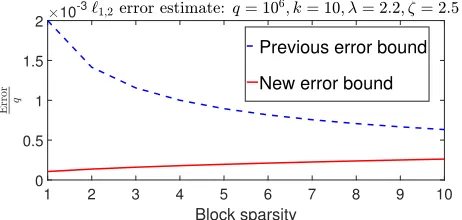
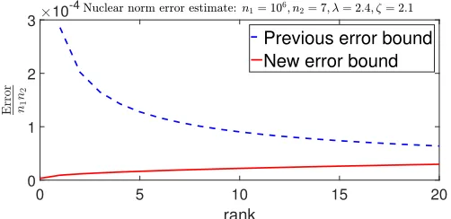
VI. NUMERICAL EXPERIMENTS

In this section, we numerically compare the new error bound of (31) against the bound (21) derived using the existing approach for various low-dimensional structures. For each test, we optimizeλandζ to minimize the right-hand side of (31). Figures 1, 2, and 3 show the proposed error bound (31) and the error estimates (24), (25), and (27), for } ¨ }1,} ¨ }1,2 and } ¨ }˚, respectively. In all cases, the sparsity/rank values are

set very small. To computeωpDpf,xq XBnqin (31), we used its upper-bound obtained via (16), [1, Equations D.6, D.10], and [19, Lemma 1]. It is clear from these figures that the new error bound outperforms the previous error bound (21) in very low sparsity/rank regimes; it should be emphasized that the curves depict the upper-bound of (31). Notice that in these three cases, both Epp

n and En

n tend to zero at large n.

Due to the varying nature of the `1 analysis case, we construct three kinds of analysis operators as follows:

1) Random 1: We first generate a pˆn Gaussian matrix with i.i.d. elements. Then, we compute its SVD as

UpˆpΣpˆnVnˆnH . Then,Σ is replaced with the matrix

Σ1:“ „

Ir 0rˆn´r

0p´rˆr 0p´rˆn´r



(39)

to get

Ω“UpˆpΣ1VnˆnH . (40)

When r “ n ďp, the constructed Ω in (40) is a tight frame. To have an analysis operator with more varied singular values, we proceed with

Ω“DpˆpUpˆpΣ1VnˆnH , (41)

whereDpˆp is a diagonal matrix. This type of matrices

is widely used as a benchmark in [11], [13], [14]. The above approach was directly adopted from [14].

2) Random 2: In this case, we simply use the Gaussian ensemble by constructing a p ˆn matrix with i.i.d. elements that each followsNp0, σ2

q. Here,σ2_implicitly specifies the range of the singular values.

3) Wavelet: We choose a redundant wavelet transform from the package SPOT [20] to construct an analysis operator. The wavelet filter is chosen from the Daubechies family and has length8. In some cases, we retain only the high-pass or low-high-pass coefficients. The rows of the wavelet operatorΩ might have non-trivial linear dependencies. For a general analysis operator Ωpˆn, we first randomly

check whetherΩSPnullpΩ_Sqis the trivial0operator or not. In

the trivial case, we regenerateS and repeat the test; otherwise, we formxvia

x“PnullpΩ_Sqw,

wherewis such thatΩx‰0. In this paper, as we would like to highlight the difference between the new error bound and the existing ones, we focus on a subclass of analysis sparse vectors. More specifically, whenever there are non-trivial linear dependencies among the columns of the analysis operator (fat or tall), we generate xaccording to the procedure explained in Section IV-A. Whenever the analysis operator is of type Random 2 (with highly coherent rows), we generate xas

x“PnullpΩ_Sqpw`αvrq, (42)

where w P Rn and α P R are arbitrary quantities and vr is the right singular vector of ΩSPnullpΩ_Sq

correspond-ing to the minimum non-zero scorrespond-ingular value (indeed, r “ rankpΩSPnullpΩ_Sqq). With this choice, the denominator of the

error bound (21) simplifies to

}ΩSPnullpΩ_Sqw`ασrur}1

}PnullpΩ_Sqw`αPnullpΩ_Sqvr}2

, (43)

where ur is the rth left singular vector of ΩSPnullpΩ_Sq.

For highly coherent analysis operators where the minimum singular value is very small, by increasingα, the denominator of the error bound (21) is likely to decrease.

For the tall analysis operators of type Random 1 in (41), we construct pairs of pΩ,xqas follows. We set

ΩS “D1U|S|ˆnVH,

Ω_S “D2U_|S|ˆnVH, (44)

where D1 andD2 are arbitrary diagonal matrices with non-negative values of size |S| ˆ |S| and |S| ˆ |S|, respectively, andU_|S|ˆn is a sub-matrix ofUpˆprestricted to the rows and

columns in S andrns, respectively. We further generatexas

x“PnullpU_|S|ˆnVH_qpw`αv_min1 q, (45)

where αą0 is an arbitrary real,w is an arbitrary vector in

Rn andvmin1 is the right singular vector corresponding to the minimum singular value σmin of U|S|ˆnVHPnullpU_|S|ˆnVH_q.

Then, the denominator of the error bound (21) becomes

}ΩSx}1 }x}2

“

}D1U|S|ˆnVHPnullpU

|S|ˆnVHq

w`ασminD1u1_min}1

}P_nullpU |S|ˆnVHq

w`αP_nullpU |S|ˆnVHq

v1

min}2 , (46)

whereu1

[image:9.612.323.553.55.162.2]

min is the left singular vector corresponding toσmin. As we have full control over α and the diagonal elements of D1, we can make the error bound (21) arbitrarily large (decreasing the diagonal elements ofD1while increasing α).

Table III compares the two error bounds for various exam-ples of tall analysis operators. We observe that our error bound (31) is considerably superior to the error estimate (21). We use three kinds of analysis operators: Random 1, 2 and Daubechies wavelet for different sparsity levels and dimensions. Notice

0 5 10 15 20

Sparsity

0 0.5 1 1.5

2 10

-3

Previous error bound New error bound

Figure 1: Two strategies of obtaining the error ofδpDpf,xqqfrom (5) in case off“ } ¨ }1. The previous and new error bounds come from (24) and (31),

respectively.

1 2 3 4 5 6 7 8 9 10

Block sparsity 0

0.5 1 1.5

2 10 -3

Previous error bound

[image:9.612.315.546.211.321.2]

New error bound

Figure 2: Comparison of the error (6) in case off“ } ¨ }1,2. The previous

and new error bounds come from (25) and (31), respectively.

that the Daubechies wavelet of size2048ˆ1024is constructed by retaining the high-pass components of a2-level Daubechies wavelet of size 3072 ˆ1024. The wavelet transformation is computed by the SPOT package [20]. The procedure of computing ωpDp}Ω¨ }1,xq X Bnq in (31) is explained in Appendix E.

In Table IV, we examine fat analysis operators including Random 1 and 2 structures, TV and Daubechies wavelet. Again, our bound (31) confirms thatUδ is close to δpDp}Ω¨

}1,xqq, while the error bound (21) is inconclusive.

Different from the above mentioned strategies for generating analysis-sparse signals, we also construct signals (shown by Random 1* in Table III and TV* in Table IV) as x “

PnullpΩ_Sqcwherecis uniformly distributed on the unit sphere.

In these cases, we observe that the error estimate (21) is effective.

VII. CONCLUSION

In this work, we presented an error estimate bound for the statistical dimension. This new bound shows that the statistical dimension is well described by its common upper-bound (5) in some settings of TV structure and `1 analysis.

APPENDIXA PROOF OFTHEOREM2 (31)

Before beginning the proof, we define some parameters and provides a proof sketch to enhance the readability. Givenλą 0, we define the parameters

α:“_Ertgs ` λ

}z0}2

, (47)

tg :“arg min

0 5 10 15 20

rank

0 1 2

3 10

-4

[image:10.612.55.306.58.180.2]

Previous error bound New error bound

Figure 3: Comparison of the error (6) in case off “ } ¨ }˚. The previous

and new error bounds come from (27) and (31), respectively.

and the function

φpgq:“dist2pg, αBfpxqq ´dist2pg,conepBfpxqqq. (49)

Notice that due to [1, Lemma C.1], whenever f is a proper convex function (as is the case in this paper),tg is well-defined

and unique. Define the event

E “ !

|tg´Ertgs| ă λ

}z0}2 )

. (50)

For fixed g, by considering the condition (30), tg is a _}z1 0}2

Lipschitz function of g[17, Lemma 3]5. Hence, by a concen-tration inequality for Lipschitz functions of Gaussian vectors (see, for example, [21, Theorem 8.40]), we get that

PtEu ěp0:“1´2e´

λ2

2 . ₍₅₁₎

Proof skech . The goal is to find an upper-bound for Eδ.

Instead of boundingEδ, we bound the expression

Edist2pg, αBfpxqq ´δpDpf,xqq “

Edist2pg, αBfpxqq ´Edist2pg,conepBfpxqqq “Eφpgq,

which is counted as its upper-bound. To reach this goal, we do the following steps:

1) WhenE holds, we find that

φ1pgq:“φpgq ´4λβdistpg,conepBfpxqqq ď4λ2β2.

2) We obtain a lower-bound for the probability of the event

φ1pgq ď4λ2β2.

3) Then, we obtain a concentration inequality for the expres-sionφ1pgqwhich is associated withEφ1pgq(see Lemma 1).

4) Combining the concentration inequality in Item 3 and the lower-bound in Item 2, we reach a contradiction unless we have that _Eφ1pgq is bounded above by a certain expression.

5) Finally, the upper-bound on _Eφpgq (and thus bound on Eδ) is directly obtained using the upper-bound on Eφ1pgq.

We now prove each of the above mentioned parts in details. Suppose that E holds. Define z˚ _{such that}

dist2pg, tgBfpxqq “ }g´tgz˚}22. (52)

5_{The proof of [17, Lemma 3] does not needz}

0to be an element ofBfpxq. Take

z“tg

αz

˚_{` p1´}tg

αqz1 P Bfpxq, (53)

wherez1is defined in (35). That this is an element ofBfpxq follows from the fact that bothz1 andz˚ are in Bfpxq, and that E implies that tg{α ă 1. Then, we can find an

upper-bound forφpgqas follows:

dist2pg, αBfpxqq ď }g´αz}22“ }g´tgz˚`tgz˚´αz}22

“ }g´tgz˚}22` }tgz˚´αz}22`2xg´tgz˚, tgz˚´αzy

ďdist2pg,conepBfpxqqq

` ptg´αq2}z1}22`2|tg´α|xg´tgz˚,z1y

ďdist2pg,conepBfpxqqq

`4λ2β2`4λβdistpg,conepBfpxqqq, (54)

where for the last inequality we use the fact thatE holds, the definition of β (34), and the Cauchy-Schwartz inequality. In the following, we obtain a lower-bound for the probability of the eventφ1pgq ď4λ2β2.

P

!

φ1pgq ď4λ2β2 )

“_P !

φ1pgq ď4λ2β2 ˇ

ˇE)_PtEu`

P

!

φ1pgq ď4λ2β2 ˇ

ˇE)_PtEu ě_PtEu ěp0, (55)

where we used (54), which implies _P !

φ1pgq ď4λ2β2 ˇ ˇE)“ 1, and (51).

In what follows, we propose a lemma that provides a relation betweenφ1pgqandEφ1pgq.

Lemma 1. Let g P Rn be a standard normal i.i.d. vector. Then, for givenλ, ζą0,

Ptφ1pgq ´Eφ1pgq ď ´γpζ`Edistpg,coneBfpxqq `2λβqu ďp0, (56)

where

γ:“ ?

72 d

ln 3

1´4e´λ₂2 _´2e´ζ₂2

,

as defined in(33).

The proof of this Lemma is postponed to Appendix C. By considering (55) and (56), we reach a contradiction unless

Erφ1pgqs ďγpζ`2λβ`Edistpg,conepBfpxqqqq `4λ2β2. (57)

By expressingφ1 in terms of φ and identifying the expected distance to the subdifferential cone as the Gaussian width, we reach the right-hand side of (31). The left-hand side is obtained by applying the Jensen’s inequality on the infimum of an affine function (which is always concave).

APPENDIXB PROOF OFTHEOREM2 (32)

structure-inducing functions including `1 analysis. However, this bound is not an error estimate for the task of predicting the phase transition (see the explanations in Remark 2) and is used in our analysis in proving (31). We proceed with an overview of the proof. We first define

φ2pgq:“distpg, αBfpxqq ´distpg,coneBfpxqq. (58)

Proof skech . The goal is to find an upper-bound for the expression

inf

tě0Edistpg, tBfpxqq ´ωpDpf,xq XB

n

q. (59)

We instead intend to find an upper-bound for_Eφ2pgq. To reach this goal, we follow the below steps:

1) Under the assumption that the eventEholds, we find that

φ2pgq ď2λβ.

2) We obtain a lower-bound for the probability of the event

φ2pgq ď2λβ.

3) We obtain a concentration inequality for the expression

φ2pgqwhich is a2-Lipschitz function ofg.

4) The concentration inequality in Item 3 and the lower-bound in Item 2 contradict each other unless we have that Eφ2pgqis bounded above by a certain expression.

We now provide the details of the proof. Suppose that (50) holds. Define z˚ _{such that}

distpg, tgBfpxqq “ }g´tgz˚}2. (60)

By recalling (53) and (47), we have that

distpg, αBfpxqq ď }g´αz}2“ }g´tgz˚`tgz˚´αz}2

ď }g´tgz˚}2` }tgz˚´αz}2ď }g´tgz˚}2`

|tg´α|}z1}2ďdistpg,coneBfpxqq `2λβ. (61)

Since _PtEu ěp0, we have that

Ptφ2pgq ď2λβu ěp0, (62)

by the argument in (55). Moreover, since φ2pgq is a 2-Lipschitz function of g, the concentration inequality for Lip-schitz functions [21, Theorem 8.40], implies that

P

!

φ2pgq ´Erφ2pgqs ď ´r )

ďe´r₈2_{. (63)}

With a change of variables, we reach:

P!φ2pgq ´Erφ2pgqs ď ´ c

8 ln 1

p0 )

ďp0. (64)

Note that (62) and (64) contradict each other unless

Etφ2pgqu ď c

8 ln 1

p0

`2λβ. (65)

Finally, by setting λ“2we reach (32).

APPENDIXC PROOF OFLEMMA1

Define the functions

f1pgq:“distpg, αBfpxqq,

f2pgq:“distpg,conepBfpxqqq,

h1pgq:“f12pgq,

h2pgq:“f22pgq, (66)

and the event

E1:“ #

f2pgq ´Ef2pgq ďζ +

. (67)

Suppose thatE andE1 hold. Then,

|h1pgq ´h1pg1q| “ |f1pgq ´f1pg1q||f1pgq `f1pg1q| ď 2}g´g1

}2pζ`Ef2pgq `2λβq, (68)

where the second inequality comes from the fact that f1 is 1-Lipschitz function of g. The last inequality is the result of

f1pgq ďf2pgq `2λβ (61). Now suppose that onlyE1 holds, Then, with the same reasoning, we have:

|h2pgq ´h2pg1q| “ |f2pgq ´f2pg1q||f2pgq `f2pg1q| ď

}g´g1

}2p|f2pgq| ` |f2pg1q|q ď2}g´g1}2pζ`Ef2pgqq, (69)

P!h1´Erh1s ď ´

r 3 ˇ ˇ ˇ ˇ

E,E1 )

ďe´

r2

72pζ`Ef2pgq`2λβq2_, P

!

h2´Erh2s ě

r 3 ˇ ˇ ˇ ˇ E1 )

ďe´

r2

72pζ`Ef2pgqq2_{. (70)}

Consequently,

Ptφ1pgq ´Erφ1pgqs ď ´ru “

P

!

h1´Erh1s ´h2`Erh2s ´4λβf2`4λβErf2s ď ´r )

ď_Pth1´Erh1s ď ´

r

3u `Pth2´Erh2s ě

r

3u`

Ptf2´Erf2s ě

r

12λβu ďP

!

h1´Erh1s ď ´

r

3 ˇ ˇ ˇE1

)

PtE1u

`_P !

h1´Erh1s ď ´

r

3 ˇ ˇ ˇE1

)

PtE1u`

P!h2´Erh2s ě

r

3 ˇ ˇ ˇE1

)

PtE1u`

P!h2´Erh2s ě

r

3 ˇ ˇ ˇE1

)

PtE1u `Ptf2´Erf2s ě

r

12λβu ď

e´

r2

72pζ`Ef2pgq`2λβq2

`2e´λ₂2

`e´ζ₂2

`e´

r2

72pζ`Ef2pgqq2

`e´ζ₂2

`e´ r 2

72ˆ4λ2β2 _ď3e´

r2

72pζ`Ef2pgq`2λβq2

`2e´λ 2 2 <sub>`2e</sub>´

ζ2

2 _,

(71)

where in the third inequality, we used

P

!

h1´Erh1s ď ´

r

3 ˇ ˇ ˇE1

) “_P

!

h1´Erh1s ď ´

r

3 ˇ ˇ ˇE1,E

)

PtEu

`P!h1´Erh1s ď ´

r

3 ˇ ˇ ˇE1,E

)

PtEu, (72)

APPENDIXD PROOF OFPROPOSITION2

The condition (30) for function f “ }Ω¨ }1 can be stated as:

Dz0: xΩTw´z0,z0y “0 :@wP B} ¨ }1pΩxq. (73)

By settingw“sgnpΩxq `v_S where}v_S}8ď1, we have:

xΩTsgnpΩxq `ΩT

SvrS,z0y “ }z0}22,

@rvS with}vrS}8ď1. (74)

Sincez0andsgnpΩxqare fixed and bothvrS and´vrS satisfy

}vrS}8ď1, it holds that:

xΩT

SvrS,z0y “0. (75)

The expressions (74) and (75) lead to:

z0PnullpΩ_Sq, (76)

xΩTsgnpΩxq,z0y “ }z0}22. (77)

To satisfy (76) and (77) simultaneously, we choose the vector

z0“ A_A1

2PnullpΩSqc0, (78)

where

A1“ xΩTsgnpΩxq,PnullpΩ_Sqc0y,

A2“ }PnullpΩ_Sqc0}22,

andc0 is an arbitrary vector. By choosingc0“ΩTsgnpΩxq, we have:

z0“PnullpΩ_SqΩ T_sgn

pΩxq (79)

APPENDIXE

NUMERICAL COMPUTATION OF THEGAUSSIAN WIDTH

The Gaussian width ωpDpf,xq XBnq plays a key role in our proposed error estimate in Theorem 2. In this appendix, we explain how to compute this quantity numerically. This approach is adapted from [11, Section B.2]. Recall that this quantity is defined as

ωpDpf,xq XBnq:“_E sup

yPDpf,xq }y}2ď1

xy,gy. (80)

By choosing a sufficiently small t, e.g.t “0.01in (11) (the rationale of this choice is discussed in [11, Section B.2]), the expression inside E can be simplified as the simple convex program:

ωpDpf,xq XBnq «_E sup

fpx`tyqďfpxq }y}2ď1

xy,gy, (81)

that can be solved using the CVX package [22].

APPENDIXF

THE WEAK DECOMPOSABILITY CONDITION FOR

`1-ANALYSIS

With a counterexample, we show that the mentioned de-composability condition does not hold in general. Let Ωpˆn

be a tall analysis operator in general position andxnˆ1 be an analysis-sparse vector such that S “ supppΩxq with |S| ě

p´n (see [14, Section 2.1]). For the weak decomposability condition of [17] to hold forpΩ,S,xq, we shall have that

Dw0P B} ¨ }1pΩxq,

@wP B} ¨ }1pΩxq: xΩTpw´w0q, ΩTw0y “0. (82)

In particular, we can set w“sgnpΩxq `v_S, wherevpˆ1 is an arbitrary vector with}v}8ď1. SincepΩxqS “0pˆ1, we

can write that

@v, }v}8ď1 :

xΩTsgnpΩxq `ΩT

SvrS , Ω

T_w

0y “ }ΩTw0}22. (83)

By setting v “ 0 and applying the result for general v, we obtain

xΩT

SvrS,Ω

T_w

0y “0, (84)

for arbitrary v with }v}8 ď1, or equivalently, for arbitrary

v. This implies that

xvrS, ΩSΩ

T_w

0y “0, (85)

or equivalently

Ω_SΩTw0“0. (86)

Asw0P B} ¨ }1pΩxq, we know thatw0“sgnpΩxq `v0S for some}v0}8 ď1.Therefore,

Ω_SΩT_SĂv0_S “ ´Ω_SΩTsgnpΩxq “ ´Ω_SΩTSsgnpΩSxq. (87)

BecauseΩis in general position,Ω_SΩT

S is invertible and we can express_Ăv0_S as

Ă

v0_S “ ´ `

Ω_SΩT_S˘´1Ω_SΩT_SsgnpΩSxq. (88)

Now, the contradiction comes from the fact that the entries

v0 in the above equation are not necessarily confined to the intervalr´1,1s. We show this by a numerical example:

x“ „

´.4472

.8944 

,Ω“ »

– 1 1 2 1 1 2 fi

fl,S“ t1,3u,S “ t2u. (89)

For the latter signal, it holds that

r

v0_S “ ´1.4, (90)

APPENDIXG

ASYMPTOTIC BEHAVIOR OFβWHENΩISGAUSSIAN ENSEMBLE

We find an upper-bound on β when the analysis operator is a Gaussian ensemble (whether fat or tall). Recall that an upper-bound forβ is obtained in (38) as follows:

βď }Ω

T

SsgnpΩSxq}2 }PnullpΩ_SqΩTSsgnpΩSxq}2

. (91)

SinceΩS is statistically independent ofΩ_S,PnullpΩ_Sqdefines

a projection onto an n´ |S| subspace that is independently and uniformly oriented with respect to v “ Ω

T

SsgnpΩSxq }ΩT

SsgnpΩSxq}2.

In addition

β ď 1

}PnullpΩ_Sqv}2

. (92)

As the relative orientation of v with respect to nullpΩ_Sq determines the upper-bound for β, we can fix v on the unit sphere and randomly rotate nullpΩ_Sq with a uniform Haar measure. Equivalently, we can fix nullpΩ_Sq and randomly selectvwith a uniform distribution on the unit sphere. In fact, the choice v “ _}gg_}

2 whereg is an i.i.d. random vector with

standard normal distribution independent of nullpΩ_Sqfulfills this requirement. With this choice, we can rewrite the upper-bound onβ as

β ď }g}2

}PnullpΩ_Sqg}2

. (93)

It is straightforward to check that }PnullpΩSq¨ }2 and } ¨ }2 are 1-Lipschitz functions. Therefore, in high dimensions, we know that }PnullpΩ_Sqg}2 and }g}2 are concentrated around

E}PnullpΩ_Sqg}2andE}g}2, respectively. Also, by [23, Corol-lary 3.2] and [21, Proposition 8.1], it holds that

E}PnullpΩ_Sqg}2ě b

E}PnullpΩ_Sqg}22´1,

E}g}2ď ?

n. (94)

Letru1, . . . ,un´|S|sbe a basis fornullpΩSq. Then, we have

E}PnullpΩ_Sqg}22“

n´|S|

ÿ

i“1

E|xui,gy|2“ n´|S|

ÿ

i“1

uTi EggTui.

(95)

Because_EggH

“I, we can now simplify (95) as

E}PnullpΩ_Sqg}

2 2“

n´|S|

ÿ

i“1

uT_iui

loomoon 1

“n´ |S|. (96)

As a result, due to (94) and (96), we reach

βď

?

n

b

n´ |S| ´1

.

APPENDIXH

ANALYSIS OPERATORS WITH ORTHOGONAL ROWS

In this section, we consider a fat analysis operator Ω P

Rpˆn that is constructed via the recipe in Item 1 of Section

VI. The result, however, holds for all analysis operators for whichΩΩT is diagonal.

WhenΩ in (41) is fat with full row-rank, we have r“p

andΩcan be expressed as

Ω“DpˆpUpˆpVnˆpT . (97)

Using MATLAB matrix notations, we have:

Ω_S “DpS,SqUpS,rpsqVprns,rpsqT,

ΩS “DpS,SqUpS,rpsqVprns,rpsqT. (98)

As a consequence, it holds that

Ω_SΩT_S “DpS,SqUpS,rpsqUTpS,rpsqDpS,Sq. (99)

SinceUpS,rpsqUT_pS,

rpsqis a submatrix ofU UT

“Ip, we

have that

Ω_SΩT_S “0. (100)

Thus, the denominator ofβ becomes

}PnullpΩSqΩ

T_sgn

pΩxq}2“ }pIn´Ω:_SΩ_SqΩTSsgnpΩSxq}2

“ }ΩT_SsgnpΩSxq}2. (101)

By checking the gradient of the cost in the optimization in the definition ofβ (numerator), we can check that

z_S “ ´pΩ_SΩT_Sq´1Ω_SΩT_SsgnpΩSxq “0 (102)

is the unique minimizer (the gradient of the cost is zero atz_S, andz_S satisfies the constraints). Also, the minimum value of the cost (value of the numerator) becomes }ΩTsgnpΩxq}2 with this choice of z_S. This reveals that the numerator of β

equals its denominator, i.e.,β“1.

ACKNOWLEDGMENT

The authors thank the anonymous reviewers for valuable comments and suggestions to improve the quality of the paper. S.Daei also wishes to thank Mohammad Ali Hoseini Nasab for fruitful discussions.

REFERENCES

[1] D. Amelunxen, M. Lotz, M. B. McCoy, and J. A. Tropp, “Living on the edge: Phase transitions in convex programs with random data,”

Information and Inference: A Journal of the IMA, vol. 3, no. 3, pp. 224–

294, 2014.

[2] V. Chandrasekaran, B. Recht, P. A. Parrilo, and A. S. Willsky, “The con-vex geometry of linear inverse problems,”Foundations of Computational

mathematics, vol. 12, no. 6, pp. 805–849, 2012.

[3] D. Donoho and J. Tanner, “Counting faces of randomly projected polytopes when the projection radically lowers dimension,”Journal of

the American Mathematical Society, vol. 22, no. 1, pp. 1–53, 2009.

[4] M. Rudelson and R. Vershynin, “On sparse reconstruction from fourier and gaussian measurements,” Communications on Pure and Applied

Mathematics, vol. 61, no. 8, pp. 1025–1045, 2008.

[5] M. Bayati, M. Lelarge, and A. Montanari, “Universality in polytope phase transitions and message passing algorithms,” The Annals of

Applied Probability, vol. 25, no. 2, pp. 753–822, 2015.

[6] M. Stojnic, “Various thresholds for `1-optimization in compressed

[7] D. L. Donoho, I. Johnstone, and A. Montanari, “Accurate prediction of phase transitions in compressed sensing via a connection to minimax denoising,” IEEE transactions on information theory, vol. 59, no. 6, pp. 3396–3433, 2013.

[8] S. Oymak and B. Hassibi, “Sharp mse bounds for proximal denoising,”

Foundations of Computational Mathematics, vol. 16, no. 4, pp. 965–

1029, 2016.

[9] M. Elad, P. Milanfar, and R. Rubinstein, “Analysis versus synthesis in signal priors,”Inverse problems, vol. 23, no. 3, p. 947, 2007. [10] Y. Gordon, “On milman’s inequality and random subspaces which

escape through a mesh in Rn,” in Geometric Aspects of Functional

Analysis, pp. 84–106, Springer, 1988.

[11] M. Genzel, G. Kutyniok, and M. M¨arz, “`1-analysis minimization and

generalized (co-) sparsity: When does recovery succeed?,”arXiv preprint

arXiv:1710.04952, 2017.

[12] P. G. Casazza, G. Kutyniok, and F. Philipp, “Introduction to finite frame theory,” inFinite Frames, pp. 1–53, Springer, 2013.

[13] M. Kabanava and H. Rauhut, “Analysis `1-recovery with frames and

Gaussian measurements,” Acta Applicandae Mathematicae, vol. 140, no. 1, pp. 173–195, 2015.

[14] S. Nam, M. E. Davies, M. Elad, and R. Gribonval, “The cosparse analysis model and algorithms,”Applied and Computational Harmonic

Analysis, vol. 34, no. 1, pp. 30–56, 2013.

[15] B. Zhang, W. Xu, J.-F. Cai, and L. Lai, “Precise phase transition of total variation minimization,” in Acoustics, Speech and Signal Processing

(ICASSP), 2016 IEEE International Conference on, pp. 4518–4522,

IEEE, 2016.

[16] R. T. Rockafellar,Convex analysis. Princeton university press, 2015. [17] R. Foygel and L. Mackey, “Corrupted sensing: Novel guarantees for

sep-arating structured signals,”IEEE Transactions on Information Theory, vol. 60, no. 2, pp. 1223–1247, 2014.

[18] E. Candes and B. Recht, “Simple bounds for recovering low-complexity models,”Mathematical Programming, vol. 141, no. 1-2, pp. 577–589, 2013.

[19] S. Daei, F. Haddadi, and A. Amini, “Exploiting prior information in block sparse signals,”arXiv preprint arXiv:1804.08444, 2018. [20] E. Van den Berg and M. Friedlander, “Spot-a linear-operator toolbox,”

URL http://www. cs. ubc. ca/labs/scl/spot, 2014.

[21] S. Foucart and H. Rauhut,A mathematical introduction to compressive

sensing, vol. 1. Birkh¨auser Basel, 2013.

[22] M. Grant and S. Boyd, “CVX: Matlab software for disciplined convex programming, version 2.1,” Mar. 2014.