Synthesizing Samples for Zero-shot Learning
IJCAI Anonymous Submission 2625
Abstract
Zero-shot learning (ZSL) is to construct recogni-tion models for unseen target classes that have no labeled samples for training. It utilizes the class attributes or semantic vectors as side information and transfers supervision information from related source classes with abundant labeled samples. Ex-isting ZSL approaches adopt an intermediary em-bedding space to measure the similarity between a sample and the attributes of a target class to perfor-m zero-shot classification. However, this way perfor-may suffer from the information loss caused by the em-bedding process and the similarity measure cannot fully make use of the data distribution. In this pa-per, we propose a novel approach which turns the ZSL problem into a conventional supervised learn-ing problem by synthesizlearn-ing samples for the unseen classes. Firstly, the probability distribution of an unseen class is estimated by using the knowledge from seen classes and the class attributes. Sec-ondly, the samples are synthesized based on the distribution for the unseen class. Finally, we can train any supervised classifiers based on the syn-thesized samples. Extensive experiments on bench-marks demonstrate the superiority of the proposed approach to the state-of-the-art ZSL approaches.
1
Introduction
Recent years have witnessed the tremendous progress of sev-eral machine learning and computer vision tasks, such as ob-ject recognition, scene understanding, and fine-grained classi-fication, together with the development of deep learning tech-niques [Krizhevskyet al., 2012; He et al., 2016]. It should be noticed that the learning scheme of them requires suffi-cient labeled samples for model training, like ImageNet [Rus-sakovskyet al., 2015]. This is affordable when dealing with common objects. However, the objects “in the wild” follow a long-tailed distribution such that the uncommon ones do not occur frequently enough, and the new concepts emerge ev-eryday especially in the Web, which makes it difficult and ex-pensive to collect and label a sufficiently large training set for model learning [Changpinyoet al., 2016]. How to train effec-tive classification models for the uncommon classes without
Elephant Panda
Lion Dolphin
Dog Monkey
……
Classes
Class Embedding Sample Embedding
Elephant
Lion
Panda Monkey Dolphin
Dog 0.14 0.49
0.66 0.72 1.06
[image:1.612.326.548.217.288.2]0.59
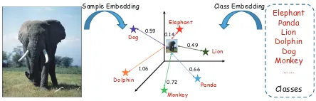
Figure 1: Framework of embedding based ZSL approaches.
using the labeled samples becomes an important and practi-cal problem and has gathered considerable research interests from the machine learning and computer vision communities. It is estimated that humans can recognize approximate
30,000 basic object categories and many more subordi-nate ones and they are able to identify new classes given an attribute description [Lampert et al., 2014]. Based on this observation, many zero-shot learning (ZSL) approach-es have been proposed [Akataet al., 2015; Al-Halahet al., 2016; Romera-Paredes and Torr, 2015; Zhang and Saligrama, 2016a]. The goal of ZSL is to build classifiers for target un-seen classes given no labeled samples, with class attributes as side information and fully labeled source seen classes as knowledge source. Different from many supervised learn-ing approaches which treat each class independently, ZSL associates classes with an intermediary attribute or seman-tic space and then transfers knowledge from the source seen classes to the target unseen classes based on the associa-tion. In this way, only the attribute vector of a target (un-seen) class is required and the classification model can be built even without any labeled samples for this class. In particular, an embedding function is learned using the la-beled samples of source seen classes that maps the images and classes into a common embedding space where the dis-tance or similarity between them can be measured. Because the attributes are shared by both source and target class-es, the embedding function learned by source classes can be directly applied to target classes [Farhadiet al., 2009; Socheret al., 2013]. Finally, given a test image, we map it into the embedding space and measure its distance to each target class and return the class with the minimal distance. An illustration of this ZSL framework is shown in Figure 1.
in-Elephant Panda
Lion Dolphin
Dog Monkey
……
Classes
Elephant Dolphin
Lion
Classifier Training
Data Synthesizing
[image:2.612.66.284.52.126.2]Prediction
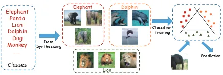
Figure 2: The proposed data synthesizing based ZSL. duced from the other seen objects, and then utilize them as supervision to guide the future classification [Miller et al., 2000]. Inspired by this observation, we propose a novel ZS-L framework based on data synthesis, as shown in Figure 2, which is totally different from existing embedding based ap-proaches. Intuitively, the embedding based ZSL can be re-garded as learning how to recognize the characteristics of an image and match them to a class. On the contrary, our frame-work can be described as learning what a class visually looks like. In particular, the proposed framework has two explic-it advantages over the embedding based framework. First-ly, the embedding based framework has to map the test im-age into an embedding space. It should be noticed that the embedding step may bring in information loss such that the overall performance of the system degrades [Fuet al., 2014; Zhang and Saligrama, 2016b; Lazaridouet al., 2015]. The proposed framework classifies a test image in the original space, which can avoid this problem. Secondly, the super-vised learning techniques has been developed rapidly in re-cent decades but it is not clear how to combine the embedding based framework with most of them. In the proposed frame-work, labeled samples for the target classes are synthesized. In this way, we turn the ZSL problem into a conventional su-pervised learning problem such that we can take advantage of the power of supervised learning techniques in the ZSL task.
In particular, we synthesize samples for each target class by probability sampling. Given the labeled samples from source classes, the conditional probability p(x|c) for each source classcis computed. Then by using the association between the source classes’ attributes and target classes’ attributes, we estimate the conditional probability for each target class by a linear reconstruction method. Next, based on the distribu-tion, some samples are synthesized. At last, any classification model can be learned in a conventional supervised way with the synthesized samples. The contributions of this paper are: 1. We propose a novel ZSL framework based on data syn-thesis. By synthesizing samples for each target class, we can turn the ZSL problem into a conventional supervised learning problem such that we can make use of many powerful tools and avoid the information loss from the embedding process.
2. Based on the structure of class attributes and image fea-tures, we adopt a simple linear reconstruction method to es-timate the conditional probability for each target class and then the samples are synthesized based on the distribution. We empirically demonstrate that the synthesized samples can well approximate the true characteristics of the target classes. To our best knowledge, this is the first work to estimate the conditional probability in the image feature space for ZSL.
3. Comprehensive experimental evidence on four bench-mark datasets demonstrates that the proposed approach can consistently outperform the state-of-the-art ZSL approaches.
2
Preliminaries and Related Works
2.1
Problem Definition and Notations
The definition of zero-shot learning is as follows. We are giv-en a set of source classesCs = {cs
1, ..., csks} andnslabeled
source samplesDs ={(xs
1,y1s), ...,(xsns,y
s
ns)}for training,
where xs
i ∈ Rd is the feature vector and ysi ∈ {0,1}ks
is the corresponding label vector which has yij = 1if the
sample i belongs to class cs
j or0 otherwise. We are given
some target samplesDt={xt
1, ...,xtnt}fromkttarget
class-esCt={ct
1, ..., ctkt}satisfyingC
s∩ Ct=∅. The goal of ZSL
is to build classification models which can predict the label c(xti)givenxti with no labeled training data for target class-es available. To associate source classclass-es and target classclass-es to facilitate knowledge transfer, for each classci ∈ Cs∪ Ct, we
assign a class attribute representationai∈Rq to it which can
be constructed from manual definition or theword2vectool.
2.2
Related Works
As introduced before, most of the existing ZSL approaches follow the embedding based framework illustrated in Figure 1. Formally, based on the problem definition and notations above, the classification methods of the previous approaches can be summarized into the general function as follows:
c(xt) =argmaxc∈Ctsim(φ(xt), ψ(ac)) (1)
whereφis the embedding function for images,ψis the em-bedding function for classes, andsim(·,·)is a similarity or distance measure function between the embedded images and classes. Existing ZSL approaches differ from each other due to different choices of these functions. For example, Lampert et al.[2014] adopted linear classifiers, identity function, and Euclidean distance respectively. Romera-Paredes and Tor-r [2015] used lineaTor-r pTor-rojection, identity function and inneTor-r product similarity. Fu et al. [2015] propose to use a deep model DeViSE [Fromeet al., 2013] for image projection and measure the similarity using the semantic manifold distance obtained from absorbing Markov chain process. Zhang and Saligrama [2016a] utilized the unit-ball constrained projec-tion, simplex constrained projecprojec-tion, and aligned inner prod-uct similarity. Some approaches have more complicated for-mulation. But we can also simplify them into the general function. For example, the formulation of Changpinyo et al.[2016] can be simplified as the combination of the linear projection by virtual classifiers, exponential transformation, and inner product similarity. Recently many ZSL approach-es have been proposed [Akataet al., 2015; Xianet al., 2016; Bucheret al., 2016; Fu and Sigal, 2016]. Because of space limit, we cannot review all of them in detail. But they mostly follow the general function above. To learn these functions, the labeled source samples are used to maximize the function:
(φ, ψ) =argmax(φ,ψ) X
isim(φ(x t
i), ψ(ac(xti))) (2)
(a) AwA (b) aPY
Figure 3: t-SNE visualization of samples from AwA and aPY datasets. Points with the same color belong to the same class. use of the unlabeled target samples to better capture the tar-get class structure [Kodirovet al., 2015; Guo et al., 2016; Zhang and Saligrama, 2016b]. However, we need to empha-size here that our work focuses on the inductive ZSL setting where no samples in target classes are available at all.
Data synthesis is an effective method to deal with the lack of training data, such as in the learning from imbalanced data problem [He and Garcia, 2009] and few-shot learning prob-lem [Milleret al., 2000; Kwittet al., 2016]. However, how to apply it to the zero-shot scenario is still a problem. Yu and Aloimonos [2010] made attempt to synthesize data for ZSL using the Author-Topic model [Rosen-Zviet al., 2010]. However, it should be noticed that their approach can only deal with discrete attributes and discrete visual features like bag-of-visual-word feature. In most of the recent ZSL set-tings, which are more practical in real world, the attributes and the visual features usually have continuous values, like the word2vecbased attributes and the deep learning based visual features. Obviously, it is unclear and difficult, if not impossible, to apply their approach to these settings, while our approach is capable of handling these practical scenarios.
3
The Propose Approach
3.1
Distribution Estimation by Reconstruction
Because of the lack of labeled samples, it is challenging to train classifiers for target classes in a conventional supervised way. To address this problem, we propose to synthesize some samples for each target class. In particular, for each target class, we wish to estimate its conditional probabilityp(x|c)
and then it is easy to synthesize samples from it by simple probability sampling. However, if we have no prior about the data distribution, the estimation will be somehow difficult. Therefore, we first briefly investigate the distribution of data. It is demonstrated that the pre-trained convolutional neu-ral network is a very powerful image feature extractor [Don-ahueet al., 2014]. Therefore, we choose the VGG-19 net-work [Simonyan and Zisserman, 2014] and use thefc7layer outputs as the image feature, which is a4,096-dimensional vector. We use the t-SNE [Van der Maaten and Hinton, 2008] to visualize the features of some classes from Animal with Attributes (AwA) [Lampertet al., 2014] and aPascal-aYahoo (aPY) [Farhadiet al., 2009], as shown in Figure 3. Here, it can be observed that the samples from the same class rough-ly form a cluster. Based on the observation, it is reasonable to assume a Gaussian distribution for each target class, i.e., p(x|c)∼ N(uc,Σc). For source classes, the mean vectoruc
ܿଵ௦ ܿଶ௦
ܿଵ௧
ܿଶ௧ 0.6
0.6 0.4
0.4
(0.6,0.4)
(0.6,0.4)
(a) Similarity
ܿଵ௦ ܿଶ௦
ܿଵ௧
ܿଶ௧
0.6
0.6 0.4
0.4
(0.7,0.3)
(0.8,0.2)
(b) Reconstruction
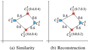
Figure 4: The numbers next to lines are the similarity between classes. The numbers in the brackets are the weights to esti-mate the parameters. In the left subfigure, only the similarity is considered such that two different target classes may have the same estimated distribution. In the right subfigure, the problem is solved since the structure of classes is considered. and the covariance matrixΣccan be easily obtained from its
labeled samples. However, for a target class, we have no more than the attribute vectorat
c and thus it is not that
straightfor-ward to estimate the parameters like the source classes. There is a saying, “one takes the behavior of one’s compa-ny.” In fact, this idea has been widely accepted by machine learning and computer vision communities. In the image clas-sification task, it is always believed that similar images (short distance between their features) are more likely to belong to the same class, which is the underlying assumption ofkNN classifier [Altman, 1992]. Analogously, in the class level, this idea seems reasonable too, indicating that similar classes should have similar properties, like the probability distribu-tion. Fortunately, the similarity between classes can be mea-sured by their attributes. One simple way to measure the sim-ilarity between a target classctand any source classcs
jis:
sj =exp(−
kat c−asjk22
ǫ2 ) (3)
whereǫis the mean value of the distances between attribute vectors of any two source classes. With the similarity, it is straightforward to estimate the distribution parameters forct
:
uct = 1
z
Xks
j=1sjuc s
j, Σct =
1
z
Xks
j=1sjΣc s
j (4)
wherez =P
jsjis a normalization parameter. In this way,
the distribution parameters for a target class can approximate-ly estimated from the information of the source classes’.
However, only considering the similarity seems too sim-ple to well capture the properties of classes. As illustrated in Figure 4(a), because two target classesct
1andct2have the
same distance to source classescs
1 and cs2, they obtain the
same parameters by Eq. (4) even if they are different. In fact, the relative structure of the classes should be also taken into account. To address this issue, we propose a reconstruction method to estimate the parameters. In particular, suppose the parameters are estimated withwjas the the weights as below:
uct= 1
z
Xks
j=1wjucsj, Σct =
1
z
Xks
j=1wjΣcsj (5)
To preserve the structure, we hope the weights are constructed such thatact ≈1
z
P
[image:3.612.74.285.58.154.2]reasonable to minimize the following reconstruction error:
min
wj
kact−Awk22+R(wj), s.t. X
jwj= 1 (6)
whereA= [as
1, ...,asks]andRis a regularization term.
Ob-viously, without proper regularization, solving the problem may assign large weights to dissimilar classes. As discussed above, we hope the similar classes have more impact on the target class. Therefore, following the locality constrained re-construction [Wanget al., 2010], we further incorporate the similaritysjas a regularization to the weights as follows:
min
wj
kact−Awk22+λ X
jwj/sj, s.t.
X
jwj = 1 (7)
Whereλis a trade-off parameter. Obviously, for dissimilar class with smallsj, minimizing the function will assign small
weightwj. The solution to the above problem is given by:
w= ((A−1a′ct)(A−1a ′
ct) ′
+λdiag(s1, ..., sks))
−1/z (8)
wherez = P
jwj is the normalization factor. Moreover,
we can take one step further to remove the influence of dis-similar source classes on the target class. In particular, we do not need to use all source classes for reconstruction. In-stead, we only need thek-nearest neighbors (k ≪ ks) ofct
inCs, denoted asN
k. In this way, the matrixAis reduced to
AN N = [asj]j∈Nk and we now just solve the subproblem to
obtain weightswj(j ∈ Nk)and simply setwj = 0(j /∈ Nk).
Then with the reconstruction based weights, the probability distribution parameters ofctcan be constructed by Eq. (5).
There is one issue worth discussing about. The covari-ance matrix contains a large number of parameters. For ex-ample, when using the4,096-dimensional deep feature, the matrix has about16 million elements. Therefore, the esti-mation of it will be complicated and very imprecise if we use the whole matrix without any constraint. Here we con-sider two convenient simplifications. The first is to assume
Σc = σcI which is the simplest approximation. In fact,
Socheret al.[2013] also assumed the isotropic Gaussian to prevent overfitting the target class. In this way, we only need to estimate the parameterσcfor each class. The second is to
assumeΣc =diag(σc1, ..., σcd)where we only consider the
diagonal elements and the other elements are assumed to be
0. This is more complicated than the isotropic variance such that it can better fit the data, but much simpler than the whole variance with orders of magnitudes and thus it is more pre-cise and less likely to overfit. In the experiment section, we consistently use the second simplification for the matrixΣc.
3.2
Classifier Training
For each target classct∈ Ct
, we obtain the estimated condi-tional probability distributionp(x|ct)∼ N(u
ct,Σct). Then
we can perform random sampling with the distribution to syn-thesizeS samples for each target class, which leads to a la-beled training set withkt× Ssynthesized samples for
learn-ing classifiers for target classes. In this way, we turn the ZSL problem into a conventional supervised learning problem. In-tuitively, any supervised classifiers can be used based on the synthesized training set, such askNN classifier, SVM, and L-ogistic Regression. Moreover, some other techniques such as
boosting methods like AdaBoost and metric learning methods can be also utilized. Compared to existing embedding based ZSL approaches, it is more straightforward to combine our approach with the supervised learning techniques such that our approach can better take advantage of the power of them. Here we can notice that our approach falls into the em-bedding based framework in an extreme case. In particular, if only one sample for each target class is synthesized and we require it to beuct and we use the1NN classifier, it
be-comes a standard embedding and similarity measure proce-dure, which is equivalent to the embedding based framework if we regard the original image feature space as the embed-ding space. However, in this way, the variance information is not considered. In addition, because only one sample is syn-thesized, it fails to provide sufficient variability, which is a critical problem for the recognition task [Kwittet al., 2016].
3.3
Discussion
Now we analyze the error bound of our approach. Denote
Dsyn as the synthesized labeled samples for target classes,
andDt
as the true samples of target classes. The true labeling function ish(x)and the learned prediction function isf(x). The distribution ofDsyn
isPsynand ofDtisPt. We define
the prediction error offinDsynandDtrespectively as:
ǫsyn(f) =Ex∼Psyn[|h(x)−f(x)|] (9)
ǫt(f) =Ex∼Pt[|h(x)−f(x)|] (10)
We can consider it as a domain adaptation problem [Ben-Davidet al., 2006]. Following the Theorem 1 in [Ben-David et al., 2006], suppose the hypothesis spaceHcontainingf is of VC-dimensiond, then with probability at least¯ 1−δ, for everyf ∈ H, the expected errorǫt(f)is bounded as follows:
ǫt(f)≤ˆǫsyn(f) +
r
4
n( ¯dlog
2en
¯
d +log
4
δ)
+dH(Dsyn,Dt) +ρ
(11)
where ˆǫsyn(f) is the empirical error of f in Dsyn, ρ =
inff∈H[ǫsyn(f) +ǫt(f)], dH(Dsyn,Dt) is the distribution
distance betweenDsyn andDt,eis the base of natural
loga-rithm, andn=ktSis the number of synthesized samples.
Our goal is to minimize ǫt(f). In fact, training classifier
withDsynis to minimizeˆǫ
syn(f). For the second term, we
can notice that the embedding based case, as discussed above, hasn = kt×1, while our approach hasn = ktS(S ≫ 1)
indicating that our approach can generalize better, which is consistent with the observation by Kwitt et al.[2016]. The third term is very important. In fact, the distribution ofDsyn
Table 1: The statistics of datasets.
AwA aPY SUN CUB
#source class 40 20 707 150 #source sample 24,295 14,140 12,695 −
#target class 10 12 10 50
#target sample 6,180 2,644 200 −
#attributes 85 64 102 312
previous works have paid little attention to evaluate the qual-ity of the attributes in a principled way. The only metric con-sidered before is the test performance. However, since the la-bels for test samples are not available, this is not feasible for real-world applications. But with this term, we can use the estimated and true distributions of source classes to compute the distance to the measure the quality of attributes, which can further guild the design and choice of the attributes.
4
Experiment
4.1
Datasets and Settings
In this paper, we adopt four benchmark datasets for ZSL. The first is Animal with Attributes (AwA) [Lampertet al., 2014] using a standard source-target split with 40 source classes and10target classes. The second is aPascal-aYahoo [Farhadi et al., 2009]. The aPascal subset has20objects from VOC challenge and the aYahoo subset has related12objects col-lected from Yahoo image search engine. Following the s-tandard setting, the aPascal provides the source classes and the aYahoo provides the target classes. The third is SUN scene recognition dataset [Patterson and Hays, 2012] which has717scenes like “airport” and “palace”. Following the s-tandard setting [Jayaraman and Grauman, 2014],707scenes are source classes and10scenes are target classes. The fourth is Caltech-UCSD-Birds-200-2011 (CUB) [Wahet al., 2011] which has200bird species. We follow the suggested split by Akata et al. [2015] which uses 150 species as source classes and 50 species as target classes. For each image, we use the VGG-19 network pre-trained on ImageNet [Si-monyan and Zisserman, 2014] as feature extractor follow-ing Zhang and Saligrama [2016a]. Specifically, we use the
4,096-dimensional output of the top fully-connected layer of the network as the feature vector. For all datasets, we utilize the attributes provided by the original datasets. The detailed statistics of these four datasets are summarized in TABLE 1.
To determine the model parameters, we employ the class-wise cross-validation method [Zhang and Saligrama, 2016a; Guoet al., 2016]. In particular, we use the labeled source classes to simulate the zero-shot setting by splitting them by class into a training set and a validation set. We use4-fold CV in this paper. After obtaining the optimal parameters, we use the whole training set to train the final model for evaluation.
4.2
Analysis
The quality of distribution estimation. We first investigate one key issue of our approach. Specifically, we use the re-lationship among class attributes to estimate the conditional distribution of each target class. So, it is very important that
true1 syn1 true2 syn2
(a) AwA
true1 syn1 true2 syn2
(b) aPY
Figure 5: Investigation on the quality of the synthesized sam-ples. True1 and true2 denote the true samples from two tar-get classes. Syn1 and syn2 stand for the synthesized samples from the estimated distributions of the corresponding classes.
1 5 10 50 100 500 1000
50 60 70 80 90
#Synthesized samples per class
Accuracy (%)
SVM−rec SVM−sim LR−rec LR−sim 1NN−rec 1NN−sim
(a) AwA
1 5 10 50 100 500 1000
35 40 45 50 55 60
#Synthesized samples per class
Accuracy (%)
SVM−rec SVM−sim LR−rec LR−sim 1NN−rec 1NN−sim
(b) aPY
Figure 6: Investigation on the influence of different classifiers (SVM, LR,1NN), different distribution estimation methods (reconstruction using Eq. (5), simimlarity using Eq. (4)), and the number of synthesized samples for each target class. the estimated distribution can approximate the true distribu-tion, or otherwise the classifiers trained with the synthesized samples perform poorly for true samples. In Figure 5, we use t-SNE to visualize the true samples from two target class-es (denoted as true1 and true2) and the synthclass-esized samplclass-es for these two classes respectively sampled from the estimated distributions (denoted as syn1 and syn2) for AwA and aPY datasets. It can be observed that the estimated distributions can well approximate the true distributions, which demon-strates that it is challenging but feasible to use class attributes to estimate the data distribution for target classes and the pro-posed reconstruction method can yield high quality estima-tion results. The other datasets and classes also have similar results, which builds a solid foundation for our approach.
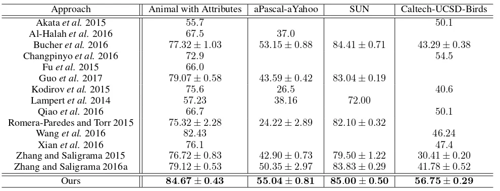
[image:5.612.320.550.215.313.2]Table 2: Zero-shot classification accuracy on four benchmark datasets.
Approach Animal with Attributes aPascal-aYahoo SUN Caltech-UCSD-Birds
Akataet al.2015 55.7 50.1
Al-Halahet al.2016 67.5 37.0
Bucheret al.2016 77.32±1.03 53.15±0.88 84.41±0.71 43.29±0.38
Changpinyoet al.2016 72.9 54.5
Fuet al.2015 66.0
Guoet al.2017 79.07±0.58 43.59±0.42 83.04±0.19
Kodirovet al.2015 75.6 26.5 40.6
Lampertet al.2014 57.23 38.16 72.00
Qiaoet al.2016 66.7 50.1
Romera-Paredes and Torr 2015 75.32±2.28 24.22±2.89 82.10±0.32
Wanget al.2016 82.43 46.24
Xianet al.2016 76.1 47.4
Zhang and Saligrama 2015 76.72±0.83 42.90±0.73 79.50±1.22 30.41±0.20
Zhang and Saligrama 2016a 79.12±0.53 50.35±2.97 83.83±0.29 41.78±0.52
Ours 84.67±0.43 55.04±0.81 85.00±0.50 56.75±0.29
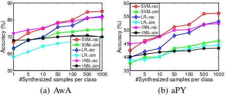
The effect of classifiers. As an important property, our approach turns the ZSL problem into the conventional super-vised learning problem such that we can utilize any powerful supervised tools. In this paper, we simply adopt three kinds of classifiers, SVM, Logistic Regression (LR) and1NN. We evaluate their performance on AwA and aPY and the results are shown in Figure 6. Typically, SVM performs better than LR and1NN especially when sufficient samples are synthe-sized. In fact, there is still difference between the estimated distribution and true distribution although the former can well approximate the latter as shown in Figure 5. Fortunately, the max-margin property of SVM seems to be to somehow robust to the distribution gap. In the future, we plan to incorporate some domain adaptation techniques [Pan and Yang, 2010] in the transductive setting to further improve the performance.
The effect of the number of synthesized samples. We further investigate the impact of the number of synthesized samples for each target class, i.e.,S, on the performance, as shown in Figure 6. Generally, the performance gets better with more synthesized samples at first since more information and variability about the target classes are given [Kwittet al., 2016]. When sufficient samples are synthesized (S >500), the accuracy stops increasing given more samples finally.
4.3
Benchmark Comparison
Now we compare the proposed approach to the state-of-the-art ZSL approaches on four benchmark datasets. Based on the above analysis, we employ SVM as the classifier. For each target class,500samples are synthesized using the re-construction based distribution. The results are summarized in Table 2. From the results, we can clearly observe the con-sistently improvements upon the state-of-the-arts given by the proposed approach, which demonstrates the effectiveness of the sample synthesis idea for ZSL. In fact, our framework is based on data synthesis and turns the ZSL problem into a con-ventional supervised learning setting, which is totally differ-ent from the embedding based framework adopted by most ZSL approaches. The results validate the superiority of the proposed framework to the embedding based framework.
Among all baselines, Zhang and Saligrama [2016a] adopts the most joint embedding function, which achieves one of the best results on AwA, aPY, and SUN. The approach of Chang-pinyo et al. [2016] constructs the synthesized classifiers in the image feature space, which is equivalent to using image feature space as the embedding space, achieving best result in baselines on CUB. However, it can be observed that they still perform worse than our approach, which is another important evidence for the superiority of the proposed approach.
Moreover, we observe that the proposed approach is even better than some transductive approaches, like Kodirovet al. [2015]. In the transductive setting, the unlabeled target sam-ples are given such that it is easier to capture the properties of target classes compared to the inductive setting where only the attributes of the target classes are available. However, be-cause an embedding is employed, the structure of data is not well preserved. It demonstrates that the embedding step may cause information loss such that the overall performance of the system degrades. Without the embedding, our approach directly synthesizes samples in the original feature space, pre-venting it from this problem, and leading to better results.
5
Conclusion
References
[Akataet al., 2015] Z. Akata, S. E. Reed, D. Walter, H. Lee, and B. Schiele. Evaluation of output embeddings for fine-grained image classification. InCVPR, 2015.
[Al-Halahet al., 2016] Z. Al-Halah, M. Tapaswi, and R. Stiefelha-gen. Recovering the missing link: Predicting class-attribute as-sociations for unsupervised zero-shot learning. InCVPR, 2016.
[Altman, 1992] N. S. Altman. An introduction to kernel and
nearest-neighbor nonparametric regression.The American Statis-tician, 46(3):175–185, 1992.
[Ben-Davidet al., 2006] Shai Ben-David, John Blitzer, Koby Crammer, and Fernando Pereira. Analysis of representations for domain adaptation. InNIPS, 2006.
[Bucheret al., 2016] Maxime Bucher, St´ephane Herbin, and
Fr´ed´eric Jurie. Improving semantic embedding consistency by metric learning for zero-shot classiffication. InECCV, 2016. [Changpinyoet al., 2016] Soravit Changpinyo, Wei-Lun Chao,
Bo-qing Gong, and Fei Sha. Synthesized classifiers for zero-shot learning. InCVPR, 2016.
[Donahueet al., 2014] J. Donahue, Y. Jia, O. Vinyals, J. Hoffman, N. Zhang, E. Tzeng, and T. Darrell. Decaf: A deep convolutional activation feature for generic visual recognition. InICML, 2014. [Farhadiet al., 2009] A. Farhadi, I. Endres, D. Hoiem, and D. A. Forsyth. Describing objects by their attributes. InCVPR, 2009. [Fromeet al., 2013] A. Frome, G. S. Corrado, J. Shlens, S. Bengio,
J. Dean, M. Ranzato, and T. Mikolov. Devise: A deep visual-semantic embedding model. InNIPS, 2013.
[Fu and Sigal, 2016] Yanwei Fu and Leonid Sigal. Semi-supervised vocabulary-informed learning. InCVPR, 2016.
[Fuet al., 2014] Y. Fu, T. M. Hospedales, T. Xiang, Z. Fu, and
S. Gong. Transductive multi-view embedding for zero-shot
recognition and annotation. InECCV, 2014.
[Fuet al., 2015] Zhenyong Fu, Tao Xiang, Elyor Kodirov, and Shaogang Gong. Zero-shot object recognition by semantic man-ifold distance. InCVPR, 2015.
[Guoet al., 2016] Yuchen Guo, Guiguang Ding, Xiaoming Jin, and Jianmin Wang. Transductive zero-shot recognition via shared model space learning. InAAAI, 2016.
[Guoet al., 2017] Yuchen Guo, Guiguang Ding, Jungong Han, and Yue Gao. Zero-shot recognition via direct classifier learning with transferred samples and pseudo labels. InAAAI, 2017.
[He and Garcia, 2009] Haibo He and Edwardo A. Garcia. Learning from imbalanced data.IEEE TKDE, 2009.
[Heet al., 2016] K. He, X. Zhang, S. Ren, and J. Sun. Deep resid-ual learning for image recognition. InCVPR, 2016.
[Jayaraman and Grauman, 2014] D. Jayaraman and K. Grauman. Zero-shot recognition with unreliable attributes. InNIPS, 2014. [Kodirovet al., 2015] Elyor Kodirov, Tao Xiang, Zhenyong Fu, and
Shaogang Gong. Unsupervised domain adaptation for zero-shot learning. InICCV, 2015.
[Krizhevskyet al., 2012] Alex Krizhevsky, Ilya Sutskever, and Ge-offrey E. Hinton. Imagenet classification with deep convolutional neural networks. InNIPS, 2012.
[Kwittet al., 2016] Roland Kwitt, Sebastian Hegenbart, and Marc Niethammer. One-shot learning of scene locations via feature trajectory transfer. InCVPR, 2016.
[Lampertet al., 2014] Christoph H. Lampert, Hannes Nickisch, and Stefan Harmeling. Attribute-based classification for zero-shot visual object categorization.IEEE TPAMI, 2014.
[Lazaridouet al., 2015] Angeliki Lazaridou, Georgiana Dinu, and Marco Baroni. Hubness and pollution: Delving into cross-space mapping for zero-shot learning. InACL, 2015.
[Milleret al., 2000] Erik G. Miller, Nicholas E. Matsakis, and Paul A. Viola. Learning from one example through shared densi-ties on transforms. InCVPR, 2000.
[Pan and Yang, 2010] Sinno Jialin Pan and Qiang Yang. A survey on transfer learning.IEEE TKDE, 2010.
[Patterson and Hays, 2012] Genevieve Patterson and James Hays. SUN attribute database: Discovering, annotating, and recogniz-ing scene attributes. InCVPR, 2012.
[Qiaoet al., 2016] Ruizhi Qiao, Lingqiao Liu, Chunhua Shen, and Anton van den Hengel. Less is more: Zero-shot learning from online textual documents with noise suppression. InCVPR, 2016. [Romera-Paredes and Torr, 2015] Bernardino Romera-Paredes and Philip H. S. Torr. An embarrassingly simple approach to zero-shot learning. InICML, 2015.
[Rosen-Zviet al., 2010] M.l Rosen-Zvi, C. Chemudugunta, T. L. Griffiths, P. Smyth, and M. Steyvers. Learning author-topic mod-els from text corpora.ACM TIST, 2010.
[Russakovskyet al., 2015] O. Russakovsky, J. Deng, H. Su,
J. Krause, S. Satheesh, S. Ma, Z.g Huang, A. Karpathy, A. Khosla, M. S. Bernstein, A. C. Berg, and Fei-Fei Li. Ima-genet large scale visual recognition challenge.IJCV, 2015. [Simonyan and Zisserman, 2014] Karen Simonyan and Andrew
Zisserman. Very deep convolutional networks for large-scale im-age recognition.CoRR, abs/1409.1556, 2014.
[Socheret al., 2013] Richard Socher, Milind Ganjoo, Christo-pher D. Manning, and Andrew Y. Ng. Zero-shot learning through cross-modal transfer. InNIPS, 2013.
[Van der Maaten and Hinton, 2008] Laurens Van der Maaten and Geoffrey Hinton. Visualizing data using t-sne.JMLR, 2008. [Wahet al., 2011] C. Wah, S. Branson, P. Welinder, P. Perona, and
S. Belongie. The Caltech-UCSD Birds-200-2011 Dataset. Tech-nical report, 2011.
[Wanget al., 2010] Jinjun Wang, Jianchao Yang, Kai Yu, Fengjun Lv, Thomas S. Huang, and Yihong Gong. Locality-constrained linear coding for image classification. InCVPR, 2010.
[Wanget al., 2016] D. Wang, Y. Li, Y. Lin, and Y. Zhuang. Rela-tional knowledge transfer for zero-shot learning. InAAAI, 2016. [Xianet al., 2016] Y. Xian, Z. Akata, G. Sharma, Q. Nguyen, M. Hein, and B. Schiele. Latent embeddings for zero-shot clas-sification. InCVPR, 2016.
[Yu and Aloimonos, 2010] Xiaodong Yu and Yiannis Aloimonos. Attribute-based transfer learning for object categorization with zero/one training example. InECCV, 2010.
[Zhang and Saligrama, 2015] Z. Zhang and V. Saligrama. Zero-shot learning via semantic similarity embedding. InICCV, 2015. [Zhang and Saligrama, 2016a] Z. Zhang and V. Saligrama. Zero-shot learning via joint latent similarity embedding. InCVPR, 2016.