warwick.ac.uk/lib-publications Manuscript version: Author’s Accepted Manuscript
The version presented in WRAP is the author’s accepted manuscript and may differ from the published version or Version of Record.
Persistent WRAP URL:
http://wrap.warwick.ac.uk/129922
How to cite:
Please refer to published version for the most recent bibliographic citation information. If a published version is known of, the repository item page linked to above, will contain details on accessing it.
Copyright and reuse:
The Warwick Research Archive Portal (WRAP) makes this work by researchers of the University of Warwick available open access under the following conditions.
Copyright © and all moral rights to the version of the paper presented here belong to the individual author(s) and/or other copyright owners. To the extent reasonable and
practicable the material made available in WRAP has been checked for eligibility before being made available.
Copies of full items can be used for personal research or study, educational, or not-for-profit purposes without prior permission or charge. Provided that the authors, title and full
bibliographic details are credited, a hyperlink and/or URL is given for the original metadata page and the content is not changed in any way.
Publisher’s statement:
Please refer to the repository item page, publisher’s statement section, for further information.
Why higher working memory capacity may help you
1
learn: Sampling, search, and degrees of approximation
2
Kevin Lloyd
Max Planck Institute for Biological Cybernetics
Max-Planck-Ring 8, 72076 T¨
ubingen, Germany
3
Adam Sanborn
Department of Psychology, University of Warwick
Gibbet Hill Road, Coventry, CV4 7AL, UK
4
David Leslie
Department of Mathematics and Statistics, Lancaster University
Lancaster, LA1 4YF, UK
5
Stephan Lewandowsky
School of Psychological Science, University of Bristol
Clifton, BS8 1TU, UK
6
Abstract
7
Algorithms for approximate Bayesian inference, such as those based on sampling 8
(i.e., Monte Carlo methods), provide a natural source of models of how people may 9
deal with uncertainty with limited cognitive resources. Here, we consider the idea 10
that individual differences in working memory capacity (WMC) may be usefully 11
modeled in terms of the number of samples, or “particles”, available to perform in-12
ference. To test this idea, we focus on two recent experiments that report positive 13
associations between WMC and two distinct aspects of categorization performance: 14
the ability to learn novel categories, and the ability to switch between different cat-15
WMC as a number of particles, we show that a single model can reproduce both 17
experimental results by varying the number of particles — increasing the number 18
of particles leads to both faster category learning and improved strategy-switching. 19
Furthermore, when we fit the model to individual participants, we found a positive 20
association between WMC and best-fit number of particles for strategy switching. 21
However, no association between WMC and best-fit number of particles was found 22
for category learning. These results are discussed in the context of the general chal-23
lenge of disentangling the contributions of different potential sources of behavioral 24
variability. 25
1
Introduction
26
How to deal with uncertainty arising from noisy and incomplete information is a 27
ubiquitous challenge for natural and artificial agents alike. Bayesian statistics pro-28
vides a rigorous system for representing and reasoning about such uncertainty, yield-29
ing a principled method for updating beliefs in the light of new evidence (Bernardo 30
& Smith, 1994). Human behavior is often well described in terms of Bayesian in-31
ference, from “low level” sensorimotor (K¨ording & Wolpert, 2004) and perceptual 32
(Yuille & Kersten, 2006) phenomena, to “high level” competencies, such as causal 33
reasoning (Griffiths & Tenenbaum, 2005), category learning (Sanborn, Navarro, & 34
Griffiths, 2010), and predictions about future everyday events (Griffiths & Tenen-35
baum, 2006; reviews include Chater & Oaksford, 2008; Sanborn & Chater, 2016; 36
Tenenbaum, Kemp, Griffiths, & Goodman, 2011). 37
How humans frequently — though by no means always (e.g., Tversky & Kahne-38
man, 1974) — achieve this consistency with Bayesian principles is less clear. Though 39
simple in principle, exact Bayesian calculations are frequently intractable in real-40
world settings, leading to a need for approximations. In statistics and computer 41
science, this challenge has been met through the development of powerful, general-42
purpose techniques for approximate Bayesian inference, such as Monte Carlo meth-43
ods (Gelfand & Smith, 1990; Robert & Casella, 2004), which allow for the practical 44
application of Bayesian methods in complex domains. 45
The practical success of these techniques has naturally led to an interest in 46
whether they also tell us something about how people reason under uncertainty. 47
logical and neural mechanisms that underlie how people process probabilistic in-49
formation (Chater & Oaksford, 2008; Doya, Ishii, Pouget, & Rao, 2007). Since 50
the aim of these algorithms is to approximate the normative solution to a com-51
putational problem — i.e., to approximate Bayesian inference — they have been 52
called rational process models when considered as candidate psychological mecha-53
nisms (Griffiths, Vul, & Sanborn, 2012; Sanborn et al., 2010). This distinguishes 54
them from traditional process models in cognitive psychology, which are typically 55
rich in postulated psychological mechanisms but often poor in terms of normative 56
foundations (cf. Anderson, 1990). 57
Importantly, Monte Carlo methods can in principle approximate probabilistic 58
inference arbitrarily well when sufficient time and memory is available, thereby pro-59
viding a benchmark for ideal performance. At the same time, these methods display 60
systematic deviations from the normative solution when resources are limited. Such 61
“qualitative fingerprints” associated with different species of approximation may 62
then be particularly illuminating when considering human cognition, where it is 63
generally assumed that information processing capacity is limited (Daw, Courville, 64
& Dayan, 2008; Gigerenzer & Goldstein, 1996; Kahneman, 2003; Simon, 1982). 65
One such limitation has long been associated with working memory (Cowan, 66
2001; Miller, 1956), defined in cognitive psychology as the memory system respon-67
sible for temporary storage and manipulation of task-relevant information (Bad-68
deley, 1992; Baddeley & Hitch, 1974). Individual differences in working memory 69
capacity (WMC), such as measured in the complex span paradigm (Daneman & 70
Carpenter, 1980), have been found to predict performance on a variety of cognitive 71
tasks, including conventional intelligence tests (Conway, Jarrold, Kane, Miyake, & 72
Towse, 2007). Indeed, WMC may account for up to one half of the variance in 73
general intelligence (Conway, Kane, & Engle, 2003). 74
However, the exact nature of the WMC limitation that underpins such individ-75
ual differences remains the subject of debate, with proposals variously emphasizing 76
decay of representations (e.g., Baddeley, Thompson, & Buchanan, 1975), resource 77
constraints (e.g., Just & Carpenter, 1992), or interference (e.g., Oberauer & Kliegl, 78
2006; see Oberauer, Farrell, Jarrold, & Lewandowsky, 2016 for a recent discus-79
sion). Indeed, opinions continue to differ as to whether working memory is best 80
conceptualized as discrete, e.g., comprising a limited number of “slots”, or as a 81
in memory (Ma, Husain, & Bays, 2014; Suchow, Fougnie, Brady, & Alvarez, 2014). 83
Our approach in the current work is to consider WMC limitations within the 84
broader context of probabilistic inference, asking whether WMC may be usefully 85
modeled as a constraint on the amount of inferential resources available. The im-86
plication is that at least in tasks involving uncertainty, enhanced performance in 87
individuals with higher WMC may be attributable to an ability to better approxi-88
mate “ideal” Bayesian solutions. 89
To begin to explore this idea, we focus on recent experiments showing positive 90
associations between WMC and performance on category learning tasks (Lewandowsky, 91
2011; Lewandowsky, Yang, Newell, & Kalish, 2012; Sewell & Lewandowsky, 2011, 92
2012). This focus is motivated by two considerations. Firstly, category learning 93
tasks are well characterized as probabilistic inference problems, requiring partic-94
ipants to reason about possible underlying category structures. Even when the 95
mapping between stimuli and category labels is deterministic, participants face 96
epistemic uncertainty regarding the nature of this mapping. Normative solutions 97
to such problems, as well as how these solutions may be practically approximated 98
— notably via Monte Carlo methods — have received substantial attention (An-99
derson, 1990; Goodman, Tenenbaum, Feldman, & Griffiths, 2008; Sanborn et al., 100
2010). We build on this previous work here. Secondly, WMC appears to be posi-101
tively associated with two distinct aspects of categorization: the ability to acquire 102
novel categories (i.e., category learning; Lewandowsky, 2011), and the ability to 103
flexibly switch between different categorization strategies (sometimes referred to as 104
“knowledge restructuring”; Sewell & Lewandowsky, 2012). Previous work has ex-105
plored how such positive associations may arise in formal category learning models 106
(Lewandowsky, 2011; Sewell & Lewandowsky, 2011, 2012) but has treated these 107
aspects of categorization separately, and via different models and mechanisms; the 108
possibility that WMC may influence both category learning and knowledge restruc-109
turing via a single mechanism has not been explored, and we seek such a common 110
mechanism in the present article. 111
The key assumptions of the current work are that individuals approximate 112
Bayesian solutions to category learning problems by sampling from probability 113
distributions (i.e., via Monte Carlo inference) and, more importantly, that an indi-114
vidual’s WMC directly translates into how many samples, or hypotheses, they are 115
the number of active hypotheses allows us to reproduce the positive associations 117
between WMC and both aspects of categorization performance — category learn-118
ing and knowledge restructuring — with a single mechanism. Before describing 119
the modeling approach and results in detail, we briefly summarize the basic ideas 120
behind Monte Carlo methods and the target experimental results. 121
1.1
Monte Carlo as a psychological mechanism
122
In the Bayesian paradigm, background knowledge gives rise to a constrained set of 123
candidate hypotheses H for the true state of nature, and to associated degrees of 124
belief P(h) in each candidate in the set h ∈ H. The sum of all beliefs about the 125
true state of nature is fixed to 1. Such “prior” beliefs are updated in the light of 126
observed data dto yield “posterior” beliefsP(h|d) via Bayes’ theorem, 127
P(h|d) = P P(d|h)P(h) h0∈HP(d|h0)P(h0)
,
where the likelihood P(d|h) quantifies how expected the data are under each can-128
didate hypothesis. 129
As we will describe in detail below, for our purposes the state of nature is the 130
true category structure that participants are required to learn; the set of candidate 131
hypotheses is the space of all possible category structures that a participant is 132
assumed to be able to generate; and the observed data are the particular category 133
instances presented to participants that they must categorize and for which they 134
subsequently receive feedback about the correct category label. 135
While Bayes’ theorem is simple to write down, it leads to complex practical 136
issues such as the source of the prior distribution, the choice of likelihood function, 137
and how to compute and summarize the posterior distribution if the hypothesis 138
space His very large — such as whenHis the space of all possible categories. 139
In Monte Carlo methods, the basic idea is to approximate the target distribution 140
P(h|d) by drawing samples from it. In other words, one representsP(h|d) with a 141
set of samples{h(i)} ∼P(h|d) from that distribution, each randomly selected with 142
a frequency proportional to its probability in the full distribution. 143
In the case where beliefs are updated sequentially as new information arrives 144
— as in the experiments we consider below, where participants receive feedback 145
trial by trial — one attempts to approximate a sequence of target distributions, 146
“particle filtering” (Doucet, de Freitas, & Gordon, 2001). As we will describe in 148
more detail, one way of promoting a good approximation to posterior distributions 149
in this instance is to propose local changes to a current hypothesish, and to accept 150
or reject the proposed variant h0 as a function of its posterior probability. This 151
latter process can be thought of in terms of continuous exploration, or search, of 152
the hypothesis space for regions of high probability. 153
These two characteristics of Monte Carlo inference — representation by a limited 154
number of hypotheses, and inference as involving an active process of exploration, 155
or search, of the posterior — draw parallels with working memory, which is typically 156
characterized not only as limited in capacity but also asactive memory (Baddeley, 157
1992). In other words, if WMC is the number of hypotheses that one can actively 158
maintain and manipulate at a given time, and if these latter processes can be cast in 159
terms of probabilistic inference, then a possible analogy between working memory 160
processes and Monte Carlo inference presents itself. 161
Of course, the idea that sampling plays a role in psychological mechanisms has 162
a long tradition in psychology (Busemeyer, 1985; Estes, 1950; Restle, 1962; Stew-163
art, Chater, & Brown, 2006), though not typically in the context of approximating 164
Bayesian inference. More recent work has explicitly considered sample-based infer-165
ence as a possible psychological mechanism (recent reviews include Griffiths et al., 166
2012; Suchow, Bourgin, & Griffiths, 2017). For example, Vul and Pashler (2008) 167
argued that the “wisdom of crowds” effect, where the error of a judgment averaged 168
over individuals is substantially smaller than the average error of individual judg-169
ments, is consistent with individuals using only a limited number of samples to form 170
estimates (cf. Lewandowsky, Griffiths, & Kalish, 2009). Other work has focused on 171
apparent suboptimalities displayed in people’s sensitivity to the ordering of infor-172
mation when they must update their beliefs over time. Such order effects have 173
been successfully captured by models employing sequential inference with limited 174
samples in a variety of domains, including change detection (Brown & Steyvers, 175
2009), garden path effects in sentence processing (Levy, Reali, & Griffiths, 2008), 176
and category learning (Sanborn et al., 2010). 177
1.2
Working memory capacity and category learning
178
Despite the central importance of both working memory and categorization in cogni-179
The nature of this relationship is of interest not only to provide further constraints 181
on adequate theories of these faculties, but also in light of recent arguments for the 182
existence of multiple categorization systems that rely to differing degrees on distinct 183
memory systems. One salient hypothesis is that category learning tasks that can be 184
solved with relatively simple, verbalizable rules (“rule-based” tasks) rely especially 185
on working memory, while tasks with solutions that generally defy description in 186
terms of simple rules (“information-integration” tasks) do not (Ashby & Maddox, 187
2005, 2011; Ashby & O’Brien, 2005). 188
In contrast to this proposal, recent studies have found a positive association be-189
tween WMC and category learning performance, regardless of whether the catego-190
rization task is rule-based (Lewandowsky, 2011) or based on information-integration 191
(Lewandowsky et al., 2012). Interestingly, WMC has also been found to be posi-192
tively associated with a somewhat distinct aspect of categorization, namely the abil-193
ity to flexibly switch between different categorization strategies (Sewell & Lewandowsky, 194
2012) — a capacity that the authors refer to as “knowledge restructuring”. These 195
apparently disparate findings, which we describe next, form the target of the current 196
work. 197
1.2.1 A positive association between WMC and category learning
198
Lewandowsky (2011) used a battery of four working memory tasks (memory updat-199
ing, operation span, sentence span, and spatial short-term memory tasks — refer 200
to the original paper for further detail and references) to measure the WMC of 201
participants before testing their category learning performance on the six classical 202
problem types of Shepard, Hovland, and Jenkins (1961) (henceforth “SHJ”). Each 203
problem type involves learning to assign each of a set of 8 stimuli to categoryAor 204
B based on their values on 3 binary dimensions (Fig. 1A); half of the stimuli are 205
assigned to category A, and the other half to category B. There are 72 possible 206
assignments that satisfy these conditions, but these reduce to 6 “types” assuming 207
interchangeability of dimensions and labels (Fig. 1B). The problem types vary with 208
respect to the number of stimulus dimensions that are relevant for classification. 209
For example, in a Type I problem, only a single dimension is relevant; in a Type 210
VI problem, by contrast, all 3 dimensions are relevant. 211
Consistent with the classical results, Lewandowsky found that the average trend 212
est, with Types II–V clustered in between (Fig. 1C). Crucially, structural equa-214
tion modeling of WMC and category learning measures also revealed that WMC 215
was positively related to category learning performance in each problem type (see 216
Lewandowsky, 2011 for details). In Figure 1D, we replot the data to show the over-217
all proportion of errors for each problem type given the median split of participants 218
into high- and low-WMC groups based on their WMC scores. There is a clear 219
trend for high-WMC participants to make fewer errors on each type of problem. 220
Entering errors into a 2 (WMC: low, high)×6 (Problem: I, II, III, IV, V, VI)×12 221
(Block: 1–12) repeated measures ANOVA confirmed that high-WMC participants 222
were more accurate than low-WMC participants (F(1,111) = 13.63, p < .01), with 223
no significant interactions between WMC and the other factors. Low-WMC par-224
ticipants made significantly more errors on each problem type, with the exception 225
of Type IV. 226
1.2.2 A positive association between WMC and knowledge
re-227
structuring
228
Sewell and Lewandowsky (2012) found that higher WMC (where WMC was as-229
sessed using the same battery of measures as in Lewandowsky, 2011) was associated 230
not only with better category learning performance, consistent with the findings of 231
Lewandowsky (2011), but also with an improved ability to switch between cat-232
egorization strategies when instructed to do so — an ability assumed to reflect 233
knowledge restructuring (Sewell & Lewandowsky, 2011). 234
Like the SHJ problems, the basic task in the studies by Sewell and Lewandowsky 235
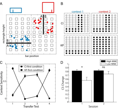
(2012) was to learn to assign stimuli to categoryAorB. Here, stimuli were rectan-236
gles that varied with respect to 3 features (height, the position a vertical bar located 237
along their base, and color). Stimuli were assigned to category A or B depending 238
on their position in stimulus space (Fig. 2A). Height and bar offset were continu-239
ous dimensions, whereas color could take only one of 2 values (e.g., blue or red). 240
Training stimuli (filled circles, Fig. 2A) were clustered into two separate regions of 241
category space, with categories arranged so that partial category boundaries (solid 242
lines, Fig. 2A) could not be integrated in a coherent manner — i.e, neither partial 243
boundary could be extended in a way that allowed accurate classification of training 244
stimuli in the other cluster, thereby encouraging co-ordination of multiple partial 245
colour
shape
size
A
B
I
II
III
IV
V
VI
Block 0
0.2 0.4 0.6
Proportion Error
I II III IV V VI
1 2 3 4 5 6 7 8 9 10 11 12
C
I II III IV V VI
Pr
opor
tion Er
ror (
O
ver
all)
0 0.1 0.2 0.3
D
Problem Type
High WMC Low WMC
*
**
**
ns*
[image:10.595.71.520.142.489.2]**
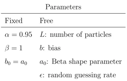
Figure 1: The 6 category learning problem types of Shepard et al. (1961).
(A) Each one of 8 stimuli is defined by its unique combination of values on three
di-mensions (e.g., color, size, and shape) that correspond to the edges of the cube. (B) In
each problem type, 4 stimuli are assigned to category A (filled circles), and the
remain-ing 4 stimuli are assigned to category B (open circles). (C) Learning curves for each
problem type, averaged over all participants, measured by Lewandowsky (data replotted
from Lewandowsky, 2011). (D) Overall proportion of errors for high- and low-WMC
participants (median split by WMC score) for each problem type. Error bars represent
B
A
D
C
bar position
rec
tangle heigh
t
A B
A
B
0 0.5 1
CI-first condition KP-first condition
Transfer Test
1 2 3 4
Con
te
xt S
ensitivit
y
CI
KP
context 1 context 2
2 1
Session 0
0.1 0.2 0.3 0.4 0.5 0.6 0.7 0.8 0.9 1
CS Change
High WMC Low WMC
[image:11.595.74.521.73.481.2]*
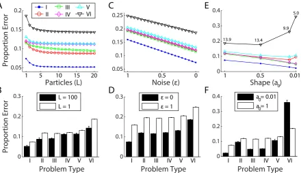
nsFigure 2: Knowledge restructuring task of Sewell and Lewandowsky (2012).
(A) Experimental stimuli. These were rectangles (two examples shown at top) that varied with respect
to their height, position of a vertically-oriented bar along their base, and color (e.g., blue or red). Stimuli
were assigned to categoryA or B depending on their position in stimulus space. Filled circles denote
training stimuli, open squares denote test stimuli, and solid lines indicate the partial rule boundaries. (B)
Ideal response profiles associated with the context-insensitive (CI; top row) and knowledge-partitioning
(KP; bottom row) categorization strategies. Shading indicates the probability with which a test stimulus
should be classified as belonging to category A (darker color indicates a higher probability). Ideal
performance in the different contexts (i.e., test stimulus presented in blue or red) is shown in the left
and right columns of panels, respectively. (C) Context sensitivity across all transfer tests for
knowledge-partitioning (KP)-first and context-insensitive (CI)-first conditions. Error bars indicate ±1 SEM. (D)
Mean absolute change in context sensitivity (CS) for participants with WMC scores in the top and
bottom quartiles (“High” and “Low” WMC, respectively) for Session 1 (i.e., between transfer tests 1 and
2) and Session 2 (i.e., between transfer tests 3 and 4). Error bars indicate +1SE. Figures A–C after
Importantly, equally good categorization performance in this task could be ob-247
tained by learning any one of a number of different strategies. For example, a 248
participant could use the color of the rectangle to decide whether height (for blue 249
rectangles) or bar position (for red rectangles) predicted category A or B — this 250
was named a knowledge-partitioning (KP) strategy. Alternatively, a participant 251
could attend to whether bar position was to the left or right of center in order 252
to then diagnose category membership based on either height or, again, bar po-253
sition — thereby ignoring the color dimension entirely. This latter was named a 254
context-insensitive (CI) strategy. 255
The crucial experimental manipulation was to encourage a participant, using 256
verbal instruction, to first learn one of these 2 strategies — by hinting that the 257
problem could be solved using bar position (for a participant assigned to the “CI-258
first” experimental group) or color (for a participant assigned to the “KP-first” 259
experimental group) — before giving the participant an unexpected instruction to 260
switch to using the alternative strategy. The degree to which participants’ predic-261
tions conformed to a CI or KP strategy could be assessed via their generalization 262
performance on a set of test stimuli (open squares, Fig. 2A), since generalization 263
performance should be either insensitive (CI strategy) or sensitive (KP strategy) 264
to the color of the presented stimuli (Fig. 2B). On the basis of their generalization 265
pattern, participants were assigned a “context sensitivity” score, summarizing the 266
degree to which their performance best conformed to a CI (context sensitivity close 267
to 0) or KP (context sensitivity close to 1) strategy. 268
Regardless of whether participants were encouraged to use a CI or KP strategy in 269
the first instance, they were able to shift between strategies without any training on 270
the novel strategy (Fig. 2C), an ability assumed to reflect knowledge restructuring 271
(Sewell & Lewandowsky, 2011). More importantly for our purposes, however, was 272
the finding of a significant positive correlation between WMC and the extent of 273
knowledge restructuring, the latter being measured in terms of the absolute change 274
in context sensitivity in each test session (see Sewell & Lewandowsky, 2012, for full 275
details of the structural equation modeling approach and results). Figure 2D shows 276
the average change in context sensitivity for participants with WMC scores in the 277
top and bottom quartiles, for Session 1 (i.e., changes between transfer tests 1 and 2) 278
and Session 2 (i.e., changes between transfer tests 3 and 4). Entering these change 279
2) repeated measures ANOVA confirmed a main effect of WMC on change in context 281
sensitivity (F(1,47) = 4.42, p < .05). High-WMC participants had significantly 282
higher changes in context sensitivity in Session 1 (t(48) = 2.81, p < .01), though 283
not in Session 2 (t(48) = 1.17,ns); we defer discussion of this, and further subtleties 284
of the experimental results, until later (see Discussion). 285
The results of Sewell and Lewandowsky (2012) thus suggest that WMC supports 286
not just standard category learning but also the flexible application of different 287
categorization strategies. 288
2
Modeling approach
289
The hypothesis of the current study was that by equating working memory capacity 290
(WMC) with the number of samples available for inference in a Bayesian category 291
learning model, positive associations between WMC, category learning, and knowl-292
edge restructuring would naturally arise, consistent with the experimental findings. 293
Our model can be described as comprising three parts: 1) a model of how 294
participants are assumed to represent categories, specified in terms of an explicit 295
process whereby categories can be constructed (i.e., a “generative model”); 2) a 296
procedure by which participants are assumed to infer categories in light of their 297
prior assumptions and the experimental stimuli; and 3) a means for translating 298
participants’ beliefs about categories into choice, i.e., a prediction of the category 299
label associated with a stimulus before receiving feedback about the true label. 300
2.1
Category representation
301
Many representational formats for categories have been discussed in the literature, 302
including rules (Bruner, Goodnow, & Austin, 1956; Goodman et al., 2008; Nosof-303
sky, Palmeri, & McKinley, 1994), prototypes (Posner & Keele, 1968; Rosch, 1973), 304
exemplars (Kruschke, 1992; Medin & Schaffer, 1978; Nosofsky, 1986), or some mix-305
ture of these (Anderson, 1991; Ashby, Alfonso-Reese, Turken, & Waldron, 1998; 306
Love, Medin, & Gureckis, 2004). In the current work, we chose to work within the 307
framework of classification and regression tree (CART) models (Breiman, Fried-308
man, Olshen, & Stone, 1984), which can be considered a type of rule-based rep-309
resentation. This choice was largely pragmatic. Firstly, CART models offer an 310
are readily described in terms of simple, verbalizable rules (i.e., “rule-based”, in 312
the terms of Ashby & Maddox, 2005) and that also suggest an ordering on rules 313
(particularly the task of Sewell & Lewandowsky, 2012; see below). Secondly, as 314
we will describe, these models are amenable to a Bayesian formulation (Chipman, 315
George, & McCulloch, 1998), which is obviously crucial for our purposes. 316
Most broadly, CART models (Breiman et al., 1984) provide a flexible method for 317
specifying the conditional distribution of a response variable (e.g., a category label) 318
given a collection of input predictors (e.g., stimulus features). In the experiments we 319
consider, category labels are always binary,y∈ {A, B}, and each stimulus to be cat-320
egorized is represented by ap-dimensional feature vectorx= (x1, x2, . . . , xp).1 The 321
models work by recursively partitioning the input space into axis-aligned cuboids 322
— imagine making a series of axis-aligned “slices” through the input space — and 323
applying a simple conditional model to each region; the sequence of partitions on 324
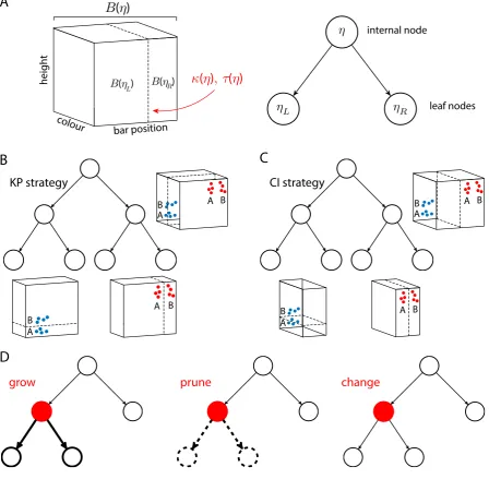
the input space can be represented as a binary tree (Fig. 3A). 325
Formally, a binary tree structureTconsists of a hierarchy of nodesη∈T. Nodes 326
with children, or leaves, are referred to as internal nodes, while nodes without 327
children are referred to asleaf nodes (Fig. 3A, right). The set of internal nodes for 328
T is denoted IT, and the set of leaves is denoted LT. Each internal node η ∈ IT
329
has exactly two children, called the left child ηL and right child ηR. Each node is 330
associated with a blockB(η)⊆Rp of the input space as follows (cf. Fig. 3A, left): 331
the root node is associated with the entire input space, while each further internal 332
node splits its block into two parts by selecting a single dimensionκ(η) ={1, . . . , p} 333
and locationτ(η) so that 334
B(ηL) =B(η)∩ {x:xκ(η)≤τ(η)} and
B(ηR) =B(η)∩ {x:xκ(η)> τ(η)}.
The block of input space associated with a node η is determined by the ranges 335
on each dimension j that it covers, and we denote the corresponding range Rηj = 336
[Rη,j−, Rη,+j ]. We call the tupleT = (T, κ, τ) thedecision tree. 337
In addition to a decision tree T with K leaf nodes, a CART model has a pa-338
rameter Θ = (θ1, θ2, . . . , θK), which associates parameter valueθk with thekth leaf 339
node. If a stimulusxlies in the region of thekth leaf node, theny|xhas distribution 340
η
ηL ηR
internal node
leaf nodes
A
B(η L) B(η R)
bar position
heigh
t
colour
A B A
B
A B
A B
A B
AB
A
B A B
B
C
B(η)
D
κ
(
η
)
, τ
(
η
)
KP strategy CI strategy
[image:15.595.75.524.78.517.2]grow prune change
Figure 3: Representing categories with a classification tree.
(A) Consider the stimulus space of Sewell and Lewandowsky (2012), which comprises 3 stimulus
dimen-sions (color, height, and bar position) and can be represented as a cube (left). A single partition of this
space into 2 subspaces can be achieved by selecting one of the stimulus dimensions (here, bar position)
and splitting the space on that dimension at a particular location. This partitioning can be represented
by a simple binary tree (right). The root nodeη (which is also an “internal” node) is associated with the
full stimulus spaceB(η). In this example, nodeηis split on the dimension corresponding to bar position
(κ(η) = bar position) at a location τ(η). This partitions the input space into two blocks, B(ηL) and
B(ηR), associated with the “leaf” nodesηLandηR. (B) Tree corresponding to a knowledge-partitioning
(KP) strategy; the initial split is on the color dimension. (D) Tree corresponding to a context-insensitive
(CI) strategy; the initial split is on the bar position dimension. (E) In the model, proposed modifications
to trees may be of 3 types, each involving the initial random selection of a node (shaded red): grow
selects a leaf node for expansion (i.e., splitting); prune selects an internal node and renders it a leaf
node by deleting all nodes below it; andchange selects an internal node and assigns it a new rule (i.e.,
f(y|θk) for some parametric family f. It is typically assumed that, conditional on 341
(Θ,T), y values within a leaf node are i.i.d., and furthermore, thaty values across 342
leaf nodes are independent. Thus, lettingnk denote the number of observations as-343
signed to thekth leaf node and lettingyk,i denote theith observation ofy assigned 344
to leafk, 345
p(y1:n|x1:n,Θ,T) = K Y
k=1 nk
Y
i=1
f(yk,i|θk), (1)
where n = PK
k=1nk is the total number of observations. As we will make more 346
precise below, for us, the parameterθk is the probability that a stimulus within the 347
kth leaf node has category label A. 348
This provides a general framework for representing categories, but we require a 349
more detailed specification for the experiments of interest. We now do this for the 350
categorization task used by Sewell and Lewandowsky (2012), described above. The 351
SHJ tasks employed in Lewandowsky (2011) are simpler and are straightforwardly 352
modeled with only minor modifications. 353
In the Sewell–Lewandowsky task, the stimulus on each trial t comprised a 3-354
dimensional input xt = (xt,1 = bar positiont ∈ R, xt,2 = heightt ∈ R+, xt,3 = 355
colort ∈ {blue = 0,red = 1}).2 On training trials, participants made a category 356
prediction before observing the binary category label yt ∈ {A, B}. The “ideal” 357
knowledge-partitioning (KP) and context-insensitive (CI) strategies which partic-358
ipants were encouraged to learn and deploy can be naturally represented in tree 359
form (Figs 3B,C). 360
In the Bayesian framework, we need to specify some prior beliefs about the 361
state of nature. In the current case, the relevant prior beliefs concern category 362
structure which, by modeling assumption, can be formalized as a prior distribution 363
on decision trees. Such a prior can be imposed implicitly by specifying a stochastic 364
process for generating such trees. Following Chipman et al. (1998), we set the prior 365
probability of a nodeη in tree structureTbeing split into children nodes to be 366
pSPLIT(η,T) =
α
(1 +dη)β
, (2)
wheredη denotes the depth of the node (the depth of the root node is zero), andα < 367
1 andβ ≥0 are parameters controlling expected tree size. Under this specification, 368
2Of course, in reality, bar position and height were much more restricted than indicated — we mean
the probabilitypSPLIT is a decreasing function of node depth, and decreases more 369
steeply for large β (cf. Figure 3 of Chipman et al., 1998). In all simulations, we 370
fix α = 0.95 and β = 1, which gives a prior mean on the number of terminal 371
nodes ≈3.7 (Chipman et al., 1998), but results are essentially identical for other 372
reasonable parameterizations. 373
In addition to a prior on tree structure T achieved through a prior on a node’s 374
probability of splitting, we need to specify the prior probability of a nodeηsplitting 375
on each stimulus dimension κ(η) = {1, . . . , p} and location τ(η). We generally 376
assume that the probability of splitting on each dimension is equal, i.e., 377
p(κ(η) =j) = 1/p, j= 1, . . . , p. (3)
Conditional on the choice of dimension, a split location is assumed to be drawn 378
uniformly from the node’s range on the relevant dimension: 379
τ(η)|κ(η) =j∼ U(Rη,j−, Rη,+j ). (4)
However, consideration of the information given to participants at the outset of 380
Sewell and Lewandowsky’s experiment leads us to a slightly different prior for the 381
root node η0. In particular, in the experiment, participants were initially told 382
that stimulus color (KP-first condition) or bar position (CI-first condition) reliably 383
indicated whether height or bar position was diagnostic of stimulus category. We 384
assume that this information is reflected in the prior probability of splitting the 385
root nodeη0 on a particular dimension. Thus, we introduce a “bias” parameter b 386
to indicate that splits of the root node η0 on one dimension should be regarded as 387
much more likely than on the others. Lettingj∗ indicate the dimension highlighted 388
by instruction, we can write this prior probability as 389
p(κ(η0)) =
b ifκ(η0) =j∗, 1−b
2 otherwise.
. (5)
Settingb <1, which would give nonzero probability to alternative splits at the root, 390
might reflect incomplete confidence in the experimenter’s instructions, for example. 391
In addition, participants were not only guided to a particular initial dimension 392
— bar position or color — but effectively also to an initial split location. Thus, 393
in the KP-first condition, attention was drawn to the color of the stimulus, while 394
was whether the bar was to the left or right of centre. We therefore assume that 396
split locations for the highlighted dimension at the root node are known. Note 397
that the question of split location is actually irrelevant in the case of the (binary) 398
color dimension since all split locations on (0,1) are equivalent in terms of the 399
resulting partition. However, this dimension can be treated as continuous for ease 400
of presentation and without consequence for modeling outcomes. 401
The preceding specifies a simple prior distribution on decision trees p(T) that 402
can be summarized as a process of deciding whether to split each node and, if so, 403
selecting a splitting dimension and location. To complete the model specification, 404
we also require a likelihood model p(y1:t|x1:t,T) that gives the conditional proba-405
bilities of stimulus labels given the tree structure. In this case, we simply assume 406
that the kth leaf node has an associated probabilityθk of generating labelA, 407
p(yt|θk,xt) =θkyt(1−θk)1−yt, (6)
and that this probability is an i.i.d. draw from a Beta distribution, 408
θk iid
∼Beta(a0, b0). (7)
Standard analytical simplification for this beta-binomial model yields the marginal 409
likelihood 410
p(y1:t|T,x1:t) =
Γ(a0+b0) Γ(a0)Γ(b0)
K K Y
k=1 Γ(nt
kA+a0)Γ(ntk·−ntkA+b0) Γ(nt
k·+a0+b0)
, (8)
where nt
kA and ntk· are respectively the number of instances of category A and
411
the total number of data points in the partition of leaf k up to trial t. Note 412
that for a given tree, this likelihood is higher for leaves assigned observations with 413
homogeneous labels (i.e., with labels that are either mostlyAor mostly B). These 414
are exactly the partitions that constitute “good” solutions to the categorization 415
problem. 416
2.2
Inference
417
Given the model specified above, we assume that participants seek to represent 418
the sequence of posterior distributions over possible trees {p(T |x1:t, y1:t)}Tt=1 as 419
Generally, a brute force procedure of enumerating all possible trees, a space which 421
dramatically increases in size with t, is not a plausible model of how participants 422
perform inference. Instead, we assume that people’s beliefs are represented by a 423
relatively small number of samples from these posterior distributions which can be 424
updated over time. In other words, we model participants as performing particle
425
filtering(Daw & Courville, 2008; Doucet et al., 2001; Sanborn, Griffiths, & Navarro, 426
2006). 427
As mentioned above, two aspects of the inference process which we now describe 428
draw parallels with working memory. Firstly, similar to the idea that there is a limit 429
on the number of items that can be held in working memory (Cowan, 2001), we 430
assume there is a bounded number of hypotheses about category structure — in this 431
case, the samples/particles which correspond to particular tree structures — that 432
can be entertained at a given time. Secondly, similar to the notion that working 433
memory isactive (Baddeley, 1992), involving the manipulation rather than merely 434
passive storage of items, we assume that inference involves a continuing process 435
whereby local transformations to current hypotheses are proposed, and which may 436
be accepted or rejected. The latter process promotes diversity in the hypothesis set 437
and continuous exploration of the hypothesis space. 438
In detail, we assume that on a given trial t, a participant’s beliefs are repre-439
sented by a small set ofLpossible trees{T(l)}L
l=1 with associated weights{w (l) t }Ll=1 440
proportional to their posterior probability. This set of trees constitutes the limited 441
set of hypotheses putatively maintained in a working memory of capacityL. With 442
the observation of the stimulus and category label on the next trialt+ 1, a proper 443
reweighting of thelth tree is given by the following update (Chopin, 2002): 444
w(l)t+1∝wt(l)p(T
(l)|x
1:t+1, y1:t+1)
p(T(l)|x
1:t, y1:t)
∝wt(l)p(y1:t+1|T
(l),x 1:t+1)
p(y1:t|T(l),x1:t)
=wt(l)p(yt+1|T(l),xt+1, y1:t). (9)
As standard within particle filtering methods (Doucet et al., 2001), this reweighting 445
process can be alternated with aresampling stage in which very unlikely trees, i.e., 446
those with very low weights, are discarded to be replaced by replicates of more 447
probable trees. A simple way of doing this is to sample Ltimes with replacement 448
(Gordon, Salmond, & Smith, 1993). 450
Additionally, this resampled particle set can then be “rejuvenated” (Chopin, 451
2002; Gilks & Berzuini, 2001), reintroducing diversity and allowing continuous ex-452
ploration of alternative solutions. This is the “active” step which, we suggest, recalls 453
conceptions of working memory as involving active manipulation of currently-stored 454
items. Specifically, we may, without altering the targeted posterior distribution of 455
interest, propose transformations of trees from a Markov chain transition kernel 456
qt+1(·|T(l)) and accept or reject these proposals such that we retain the appro-457
priate stationary distribution p(T |x1:t+1, y1:t+1). Closely following the transition 458
kernel suggested by Chipman et al. (1998), we consider the scheme where for each 459
tree {T(l)}, a new treeT(l)∗ is proposed by randomly choosing among 3 possible
460
transformations (Fig. 3D): 461
1. GROW: Randomly select a leaf node, then draw a splitting dimension and 462
location from the prior (Equations (3) and (4)). Not permitted if the split 463
leads to an empty node (i.e., a partition with no assigned data points). 464
2. PRUNE: Randomly select an internal node, then turn it into a leaf node by 465
deleting all nodes below it. Not permitted if the tree comprises only the root 466
node. 467
3. CHANGE: Randomly select an internal node, then randomly reassign it a 468
splitting dimension and location by a draw from the prior. Not permitted 469
if the reassigned split is inconsistent with splits of nodes below the selected 470
node. 471
This proposed tree T(l)∗ is then accepted with probability
472
α(T(l),T(l)∗) = min
(
1,p(T
(l)∗|x
1:t+1, y1:t+1)/qt+1(T(l)∗|T(l))
p(T(l)|x
1:t+1, y1:t+1)/qt+1(T(l)|T(l)∗) )
, (10)
as per the standard Metropolis-Hastings algorithm (Gelman, Carlin, Stern, & Ru-473
bin, 2004). This simple “resample-move” algorithm (Chopin, 2002; Gilks & Berzuini, 474
2001) is summarized in Algorithm 1. 475
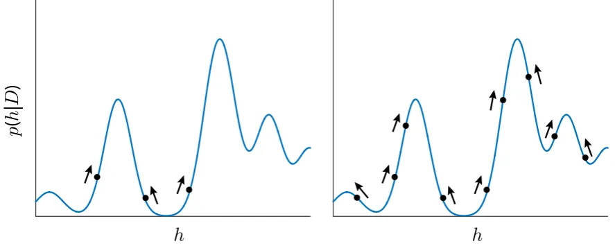
Why might the number of samples/particles be expected to influence category 476
learning? The basic intuition comes from viewing the category learning process 477
as one ofsearch (Fig. 4). In particular, “good” category structures are those that 478
partition stimuli into regions with homogeneous labels (A or B), and these are 479
Algorithm 1 Resample-Move.
Draw Lsample trees from the prior p(T) and initialize all weights tow(l)0 = 1/L.
for each trialt = 1,2, . . . do
Update each particle’s weight wt(l)∝w(l)t−1×p(yt|T(l),xt, y1:t−1).
Resample particles proportional to their updated weights{w(l)t }L l=1.
Reset each of the (resampled) particle’s weights to wt(l)= 1/L.
for each particle l = 1,2, . . . , L do
Propose a new tree T(l)∗ ∼q
t(·|T(l)).
Accept the proposal with probability α(T(l),T(l)∗) (as in Eq.(10)).
end for
end for
inference procedure we consider, the population of particles will seek out regions 481
of high posterior probability, and the rate at which these regions are found may 482
plausibly depend on the number of particles. 483
So far, we have suggested a particle filtering scheme for representing a sequence 484
of posterior distributions over category structures, where that structure is assumed 485
to be specified by a classification tree. However, we have not yet addressed the issue 486
of strategy switching. Thus, in the Sewell–Lewandowsky experiment, participants 487
were able to immediately switch between different categorization strategies when 488
instructed to do so, and in the absence of further training. 489
We model such switches as a simple reweighting operation on the set of trees. 490
Take the specific example where a participant has initially been encouraged to 491
use the CI strategy and after t training sessions has in mind the set of weighted 492
trees {T(l), w(l)
t }Ll=1 approximating the target distribution under the prior appro-493
priate to the CI strategy. We denote this target distribution pCI(T |x1:t, y1:t). The 494
experimenter then instructs the participant to change to using the KP strategy. 495
Assuming that the set of trees remains fixed, the associated tree weights now need 496
to be changed to reflect the new target distribution pKP(T |x1:t, y1:t). This can be 497
achieved by an importance weighting step, treating pCI(T |x1:t, y1:t) as the impor-498
tance distribution. In particular, denoting a particle’s weight before and after the 499
h
p
(
h
|
D
)
[image:22.595.79.523.224.403.2]h
Figure 4: Category learning as search.
In the formulation here, category learning is conceptualized as a process of search for
category structuresh∈ H that have a high posterior probability, p(h|D), given both the
prior distribution on category structures and the observed data, D. In the sample-based
inference procedure considered, this search is enacted by a particle set (black circles)
whose positions may be changed through the acceptance of proposed local changes to
the corresponding category structure. Proposals that result in a category structure with
higher posterior probability (arrows) will be accepted more often. With a larger number
of particles (right), this search may be more efficient, in that high probability structures
wt(l)+∝w(l)t − pKP(T
(l)|x
1:t, y1:t)
pCI(T(l)|x1:t, y1:t)
, (11)
which, under the specified model, becomes particularly simple: 501
wt(l)+∝
wt(l)−×(1−2b)/b ifκ(η0) = bar position,
wt(l)− ifκ(η0) = height,
wt(l)−×b/(1−2b) ifκ(η0) = color.
(12)
To switch in the reverse direction — from the KP to CI strategy — the appropri-502
ate reweighting involves the ratio pCI(T(l)|x1:t, y1:t)/pKP(T(l)|x1:t, y1:t), with the 503
appropriate alterations made to Equation 12. 504
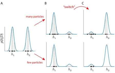
Again, why might a greater number of particles improve ability to switch be-505
tween strategies? Consider the cartoon example in Figure 5A, depicting the pos-506
terior probability P(h|D) of different possible category structures h ∈ H given a 507
stimulus setD. In this example, two particular category structures,h1 and h2, are 508
most probable, and equally so, and we can think of these as being two equally valid 509
categorization strategies, as in the Sewell–Lewandowsky task. Again, this proba-510
bility distribution will be represented by a set of particles with locations (i.e., par-511
ticular category structures) drawn from this distribution, along with corresponding 512
weights that are proportional to the posterior probabilities of those locations. 513
Now assume that the effect of an instruction to use a particular strategy is 514
to increase the posterior probability of category structures that accord with that 515
strategy, in this case those in the region ofh1 (Fig. 5B). Such a change in posterior 516
distribution, driven by the different priors underlying the distinct strategies, is 517
exactly what we assumed when suggesting that strategy-switching is mediated by a 518
reweighting of particles (see above). Depending on the number of particles available, 519
how well this collection of particles represents the true posterior distribution — 520
especially in regions of lower probability — may differ. With a sufficiently large 521
number of particles, at least some particles should be allocated to regions of lower 522
probability, such as aroundh2(Fig. 5B, upper). However, with a decreasing number 523
of particles, representation of the posterior distribution may become impoverished 524
to the extent that such regions of low probability may not contain any particles 525
at all (Fig. 5B, lower). In other words, the shift in “mental set” associated with 526
a switch in categorization strategy is here implemented by a change in posterior 527
to depend in some sense on the diversity of the current hypothesis set. 529
The possible relevance to knowledge restructuring is what these different degrees 530
of approximation to the true posterior may entail when instructed to switch catego-531
rization strategy. Intuitively, if fewer resources have been devoted to representing 532
alternative strategies in the first place, however unlikely, then it may be more dif-533
ficult to entertain these alternatives when instructed to do so. In our particular 534
formulation of the switching process, we considered a simple formulation in which 535
the immediate effect of an instruction to switch strategy is that the locations of 536
the particles remain the same, but the relative weightings of particles are updated 537
according to the new posterior distribution (Fig. 5C). In particular, if there are 538
particles located in the region of h2, these will immediately be updated (Fig. 5C, 539
upper), and the new categorization strategy can be immediately deployed. By con-540
trast, if there are no particles located in the region ofh2, no up-weighting can occur 541
and the alternative strategy is initially unavailable (Fig. 5C, lower). 542
2.3
Choice
543
We have so far described a process for performing inference (i.e., particle filtering) 544
under an assumed generative model for the structure of categories (i.e., CART). 545
What is still missing is a model of how participants finally generate a guess about 546
a stimulus’ category label before they receive feedback in the form of the true 547
label. We consider two possible choice rules: one in which a participant chooses 548
the category label with the highest probability (“maximum-probability rule”), and 549
another in which a participant chooses a category label stochastically in accord 550
with their probabilities (“probability-matching rule”). Since there is no explore-551
exploit dilemma in the categorization tasks we consider — full information about 552
the correct label is always received, regardless of choice — participants should 553
always select the label the think is most likely (i.e., maximum-probability rule). 554
On the other hand, given that probability-matching behavior has sometimes been 555
observed in this domain (e.g., Estes, Campbell, Hatsopoulos, & Hurwitz, 1989; 556
Gluck & Bower, 1988), we considered it possible that participants also used this 557
strategy, despite it being suboptimal in the tasks considered. 558
From the above, a sample-based approximation to the predictive probability 559
p
(
h
|
D
)
h
h
h
h
h
h
h
h
h
h
“switch”
many particles
few particles
[image:25.595.72.522.68.352.2]A
B
C
Figure 5: Particle diversity and flexibility of behavior.
Cartoon of how different numbers of particles affect the model’s ability to switch between
different categorization strategies. (A) Given the observed data D, comprising a set of
stimuli and their category labels, there is a posterior distribution P(h|D) over the set of
possible category structures h ∈ H. Here, two particular category structures h1 and h2
are equally probable, and can be considered as two equally valid categorization strategies.
The distribution can be approximated by a set of particles, where each particle has a
par-ticular location (circles), corresponding to a category structureh, and a weight, which is
proportional to the posterior probability (vertical, dashed lines). (B) The instruction to
use a particular strategy is conceptualized as biasing the posterior distribution so that
particular category structures are more probable, in this case category structures in the
region of h1. Whether regions of lower probability are represented in the approximation
depends on the number of particles: if there are many particles, some are likely to be
located in regions of lower probability, such as around h2 (upper); if there are fewer
par-ticles, there may be no particles in this region (lower). (C) The instruction to switch
strategy is conceptualized as leading to a change in the posterior distribution, and a
cor-responding change in the particle weights (upper); however, in the case of fewer particles,
there may be no particles immediately available to represent the change in distribution
p(yt+1 =A|x1:t+1, y1:t) = X
T
p(yt+1 =A|x1:t+1, y1:t,T)p(T |x1:t, y1:t)
≈ 1
L
L X
l=1
p(yt+1=A|x1:t+1, y1:t,T(l))
= 1
L
L X
l=1
Eθk|x1:t+1,y1:t,T(l)[θk], (13)
noting that 561
p(yt+1 =A|x1:t+1, y1:t,T(l)) = Z
p(yt+1 =A|x1:t+1, y1:t, θk,T(l))p(θk|x1:t+1, y1:t,T(l))dθk
=
Z
θk p(θk|x1:t+1, y1:t,T(l))dθk
=Eθk|x1:t+1,y1:t,T(l)[θk].
Equation (13) simply says that an approximation to the predictive probability in 562
this case is given by an unweighted average of posterior means forθk, where kfor 563
thelth particle is the index of the leaf node relevant to the inputxt+1 inT(l). For 564
the leaf model used in the current case, the posterior mean is given by 565
Eθk|x1:t+1,y1:t,T(l)[θk] = nt
kA+a0
nt
k·+a0+b0
, (14)
where, again, nt
kA and ntk· are respectively the number of instances of category A
566
and the total number of data points in the partition of leafk up to trialt. 567
The deterministic maximum-probability rule would choose the category label 568
with the highest predictive probability, but more generally we consider the-greedy 569
form 570
Pt+1(A) = (1−)1p(ye t+1=A)>p(ye t+1=B)+ 0.5, (15)
wherePt+1(A) is the probability of guessing categoryA on trial (t+ 1),pe(yt+1) is
571
shorthand for the sample-based approximation given in Eq. (13),is the probability 572
of guessing a category label according to the flip of a fair coin, and1·is the indicator
573
function. In other words: choose the most probable label with probability (1−), 574
or with probability simply flip a coin. When = 0, we recover the deterministic 575
case. 576
Pt+1(A) = (1−)pe(yt+1=A) + 0.5, (16)
so that the probability of guessing a category label is a linear combination of its 578
predictive probability pe(yt+1) (again, using shorthand for the probability given in
579
Eq. (13)) and the guessing rate ; strict probability-matching is obtained when 580
= 0. 581
Given that sample-based inference will itself tend to introduce stochasticity, we 582
should comment on the addition of a guessing rate , which, for >0, will provide 583
an additional source of variability. Briefly, our motivation was simply the (common) 584
observation that model fit was improved by including this parameter; the behavior 585
of participants tended to exhibit levels of variability beyond what our model would 586
generate with = 0, even with a single particle. As such,captures our ignorance 587
about such variability, which may arise from sources distinct from sample-based 588
inference (e.g., lapses in attention, lack of motivation, etc.). Of course, the price 589
to be paid for this improvement in fit, as we will see below, is that apportioning 590
responsibility for behavioral variability to different components of the model — 591
inference versus choice — becomes all the more difficult. 592
2.4
Model-fitting and analysis
593
Models of varying degrees of complexity were fit to the data by finding the com-594
bination of the parameters of our category-learning model (described above) that 595
maximized the likelihood of the observed sequence of category predictions. Models 596
varied in the number of parameters to be fit, lying on a spectrum from the simplest 597
case, which required that all participants be fit by a single set of parameters, to 598
the most complex case, in which each participant was fit with a separate set of 599
parameters. Formally, denoting an observed sequence of predictions over T trials 600
byc1:T and the full set of parameters by Φ ={L, b, α, β, a0, b0, }(see Table 1), the 601
general aim was to find the (free) parameters Φ that maximized the probability 602
p(c1:T|Φ,x1:T, y1:T−1) = T Y
t=1
p(ct|Φ,x1:t, y1:t−1),
with the trial-by-trial probabilities extracted from Eq. (15) or Eq. (16), as appro-603
Best-fit parameters for a given model were defined as those maximizing the aver-605
age likelihood in a grid search. The grid was defined as follows: number of particles 606
Llogarithmically spaced on the interval [1,100], yielding thirty-four values; guessing 607
rate uniformly-spaced ∈(0,0.02,0.04, . . . ,0.2); and shape a0 ∈ (0.01,0.1,0.5,1). 608
In the knowledge-restructuring case, we also included three possible values of bias, 609
b∈ {0.5,0.75,0.9}. The grid values were chosen to reflect our a priori assumptions 610
about plausible parameter values. That is, we expected participants to be more 611
plausibly modeled as instantiating relatively few particles (hence the logarithmic 612
scale), and as expressing noise levels in the lower range (hence the upper limit of 613
0.2 on the guessing rate). The choice of comparatively finely-spaced values was 614
motivated by the expectation thatLandwould at least partly trade off with each 615
other, so effort was made to make the resolution of these parameters comparable in 616
order to minimize the possibility of bias. In addition, we included the case where 617
the number of particles was set to a much larger number (L = 10,000); this was 618
to provide a comparison model that approximated the full posterior distribution 619
much more closely than when the number of particles was more restricted. 620
Since the estimate of the likelihood was generally less reliable with fewer parti-621
cles (due to greater variability in the algorithm’s behavior), the number of simula-622
tion runs was chosen so that an “effective” number of particles would be constant, 623
thereby facilitating a fair comparison between the fits of different numbers of par-624
ticles. We set the effective number of particles to 1000, so that the number of 625
simulation runs was determined by rounding to the nearest integer the result of 626
1000/L (i.e., the 1-particle case was run 1000 times, the 100-particle case was run 627
10 times, etc.). 628
As mentioned in Section 2.3, we additionally compared two different choice mod-629
els. Modulo the effect of the guessing rate, either a stimulus was deterministically 630
assigned to the most likely category (maximum-probability choice rule), or it was 631
probabilistically assigned to a category in proportion to that category’s predictive 632
probability (probability-matching choice rule). 633
In evaluating the fit of different models, we used the Bayesian information cri-634
terion (BIC) to select the best-fitting model (Schwarz, 1978); that is, we chose the 635
modelM for which the quantity BIC≡ −log(P(D|M,ΦˆM)) +12klog(n) was mini-636
mized, whereP(D|M,ΦˆM) is the value of the likelihood function (see above) given 637
estimated parameters in the model, and n is the number of data points (i.e., the 639
number of trials). 640
To assess relationships between best-fitting model parameters and participants’ 641
WMC scores, we used two methods. The simplest was simply to measure the 642
correlation between these and determine whether the correlation was significantly 643
different from zero. While this method is straightforward, the strength of the 644
correlation can be reduced by both imprecision in estimating the best-fitting model 645
parameters, as well as tradeoffs between parameters in fitting the data. While these 646
issues cannot be entirely avoided, we developed a second measure to mitigate them 647
which involved estimating a function that mapped WMC scores to a particular 648
parameter of interest as part of the fitting procedure. To do so, we used BIC scores 649
to compare slope-intercept models (in which the parameter of interest was a linear 650
function of the individual WMC scores) against intercept-only models (in which 651
the parameter was fixed across participants and thus did not depend on WMC 652
scores). In cases in which there is a relationship between a parameter and WMC 653
scores the slope-intercept model should perform better as the slope helps to capture 654
that relationship. Our second measure helps address imprecision in estimating 655
parameters because the parameters fit in the slope-intercept model are the best-656
fitting values that are consistent with a relationship with WMC, so if the individual 657
parameters are somewhat imprecise but still consistent with a relationship to WMC, 658
then the slope-intercept model would still perform best. Additionally, because 659
of the concern of parameter tradeoffs in fitting the data, we allowed the other 660
parameters in both the slope-intercept and intercept-only models to freely vary, so 661
that these other parameters could trade off against the linear relationship between 662
the parameter of interest and WMC in the way that allowed the best fit to the 663
data. (ADAM HERE?) When comparing details of model fit with a participant’s 664
WMC score, we always used for the latter the average of that participant’s scores 665
over the battery of working memory tasks used in Lewandowsky (2011) and Sewell 666
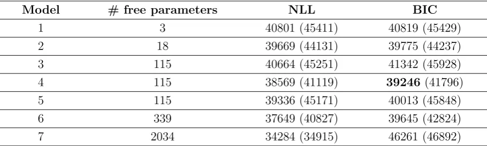
Table 1: Model parameters. See text for details.
Parameters
Fixed Free
α = 0.95 L: number of particles
β = 1 b: bias
b0 =a0 a0: Beta shape parameter
: random guessing rate
3
Results
668
3.1
Category learning
669
3.1.1 Simulations
670
Both Lewandowsky (2011) and Sewell and Lewandowsky (2012) found that working 671
memory capacity (WMC) was positively correlated with category learning perfor-672
mance, such that participants with higher WMC tended to make fewer catego-673
rization errors. We hypothesized that a greater number of particles would have a 674
similar effect because, on average, one might expect the search for a “good” (i.e., 675
more probable) category structure to progress faster, and with less chance of get-676
ting stuck at local maxima, with a higher number of particles (Fig. 4). Here, we 677
focus on simulating the classical SHJ tasks used by Lewandowsky (2011). Since 678
we always found that the probability-matching choice rule yielded better fits to the 679
data than the maximum-probability rule (see Table 2 below), the simulation results 680
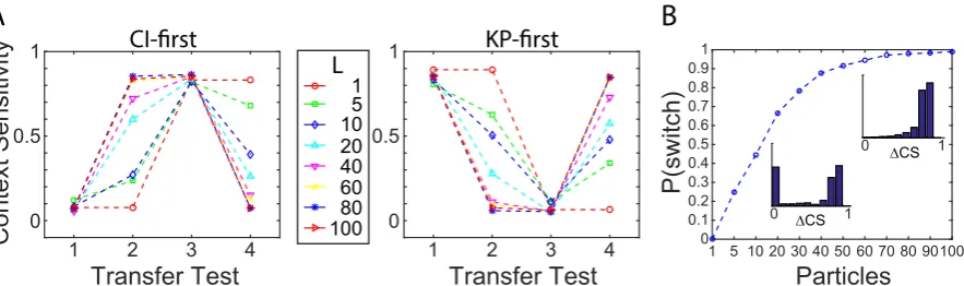
always reflect use of the former. 681
Figure 6A shows the overall average error rate for simulations as the number of 682
particles is increased from 1 to 20 while keeping other parameter values fixed (a0= 683
1, = 0); each data point represents 113 simulation runs, where each simulation 684
run uses a stimulus sequence of 192 trials observed by one of the 113 participants 685
in Lewandowsky (2011). For each problem type, increasing the number of particles 686
does indeed lead to a decrease in the average proportion of errors, though the size 687
of this effect is rather modest and quickly asymptotes (Note that the x-axis here 688
indicates the number of particles — not block number, as in Fig. 1C). 689