A robust modulation classification method using convolutional neural networks

R E S E A R C H

Open Access

A robust modulation classification

method using convolutional neural

networks

Siyang Zhou

, Zhendong Yin

, Zhilu Wu

, Yunfei Chen

, Nan Zhao

and Zhutian Yang

Abstract

Automatic modulation classification (AMC) is a core technique in noncooperative communication systems. In particular, feature-based (FB) AMC algorithms have been widely studied. Current FB AMC methods are commonly designed for a limited set of modulation and lack of generalization ability; to tackle this challenge, a robust AMC method using convolutional neural networks (CNN) is proposed in this paper. In total, 15 different modulation types are considered. The proposed method can classify the received signal directly without feature extracion, and it can automatically learn features from the received signals. The features learned by the CNN are presented and analyzed. The robust features of the received signals in a specific SNR range are studied. The accuracy of classification using CNN is shown to be remarkable, particularly for low SNRs. The generalization ability of robust features is also proven to be excellent using the support vector machine (SVM). Finally, to help us better understand the process of feature learning, some outputs of intermediate layers of the CNN are visualized.

Keywords: Robust automatic modulation classification, Convolutional neural networks, Deep learning, Feature learning

1 Introduction

Automatic modulation classification (AMC) that identi-fies the modulation type of the received signal is an essen-tial part of noncooperative communication systems. The AMC plays an important role in many civil and military applications such as cognitive radio, adaptive communi-cation, and electronic reconnaissance.

In these systems, transmitters can freely choose the modulation type of signals; however, the knowledge of modulation type is necessary to the receivers to demodu-late the signals so that the transmission can be successful. AMC is a sufficient way to solve this problem with no effects on spectrum efficiency

AMC algorithms have been widely studied in the past 20 years. In general, conventional AMC algorithms can be divided into two categories: likelihood-based (LB) [1] and feature-based (FB) [2]. LB methods are based on the

*Correspondence:[email protected]

1_{School of Electronics and Information Engineering, Harbin Institute of} Technology, No. 92 West Dazhi Street, Nangang District, Harbin, China Full list of author information is available at the end of the article

likelihood function of the received signal, and FB methods depend on feature extraction and classifier design.

Although LB methods can theoretically achieve the optimal solution, they suffer from high computational complexity and require prior information from transmit-ters. In contrast, FB methods can obtain suboptimal solu-tions with much smaller computational complexity and do not depend on prior information.

Since the prior information required by LB methods is often unavailable in practice, researchers have paid more attention to FB methods over the past two decades. The two most important parts of FB methods are feature extraction and classifier. Various types of features have been studied and used in AMC algorithms. For exam-ple, instantaneous features [3, 4] were extracted from the instantaneous amplitude, frequency, and phase in the time domain. Transformation-based features were calcu-lated from Fourier and wavelet transforms [5, 6]. The high-order cumulant (HOC) features [7, 8] are statisti-cal features obtained from different orders of cumulants from the received signals. Additive white Gaussian noise (AWGN) can be completely mathematically eliminated in

HOC features. Cyclostationary features are based on the spectral correlation function (SCF) derived from Fourier transform of the cyclic autocorrelation function [9, 10]. The highest values of SCF for different cyclic frequencies are taken by the cyclic domain profile and used to train the classifiers.

The classifier is another important part of FB methods. The decision tree [3] is the most widely applied linear clas-sifier in early years. Linear clasclas-sifiers are notably easy to implement but not feasible for linearly inseparable prob-lems. Many nonlinear classifiers are applied in AMC, e.g., K nearest neighbor [11], neural networks [12], and sup-port vector machine (SVM) with kernels [13]. SVM is considered to have advantages when the number of sam-ples is limited and can provide better generalization ability at the same time. Thus, SVM has become the most useful classifier for AMC problems in recent years.

The performance of FB methods primarily depends on the extracted feature set. Features must be manu-ally designed to accommodate the corresponding set of modulation and channel environment and may not be feasible in all conditions. Moreover, looking for effective features requires great consideration. Considering these factors, deep learning (DL) methods, which can auto-matically extract features, have been adopted. DL is a branch of machine learning and has achieved remarkable success because of its excellent classification ability. DL has been applied in many fields such as image classifi-cation [14] and natural language processing [15]. Several typical DL networks such as a deep belief network [16], stacked auto encoder [17], and convolutional neural net-work (CNN) [18] have been applied in AMC. DL networks are commonly deployed as classifiers in most current DL methods. They address different aforementioned features. The classification accuracy of DL methods has proven to be higher than other classifiers, particularly when the signal-to-noise ratio (SNR) is low.

Currently, most DL-based AMC methods are still imple-mented in two steps: preprocessing and classification. The preprocessing can be either transforms or feature extraction. DL networks are applied as classifiers to han-dle preprocessed signals. An AMC method based on DBN was proposed in [19]. The modulation set consists of 11 modulation types. Spectra in different orders are calculated for the classification. The classification accu-racy is higher than that of conventional neural networks. Zhu and Fujii proposed a high-accuracy classification scenario [20], where 10 different HOC features were extracted from 5 modulation types, and SDAE was used to classify these features. Mendis et al. [16] proposed a DBN-based method using the SCF of the received sig-nals. The classification accuracy is 95% when the SNR is

−2 dB. Dai et al. [17] proposed an interclass classifica-tion method using the ambiguity funcclassifica-tion of the signal.

Stacked sparse autoencoders are deployed as its classi-fier. The modulation set contains 7 modulation types, and the generalization ability is also studied. The classifica-tion accuracy reaches 90.4% when the SNR is between

−10 and 0 dB. O’Shea et al. [18] trained the CNN with the received based band signals directly, and the classifi-cation accuracy was higher than those trained by HOC features. Some features extracted by CNN were also dis-played. A heterogeneous model based on real-measured data is proposed in [21], and the performance is enhanced by combining CNN with recurrent neural networks.

The existing methods are all based on the assumption that the SNRs of training and testing are equal. How-ever, the result of SNR estimation is often inaccurate in practice, the actual channel SNR may also be unstable or rapid varying under certain conditions. In this case, cur-rent schemes are often lack of generalization ability. To solve this problem, a CNN-SVM model for AMC is pro-posed in this paper. Considering the advantages of the powerful capability of feature learning for deep learn-ing networks, CNN is deployed to explore new features that are suitable for classification under various SNRs. In this paper, CNN directly handles the received signals at mid-frequency from −10 to 20 dB, and is able to create new features robust to SNR variation. The generalization ability of AMC under varying SNR conditions can be sig-nificantly improved by these features. The advantages and contributions of our proposed method in this paper are stated as follows:

• Most current methods identify a limited set of modulation types, whereas the set of modulations considered in this paper is more complicated and contains 15 different types in total.

• Received signals are directly handled by the DL network at intermediate frequency (IF); however, most existing methods still require extra processing or transformation before classifying signals.

• The method can provide an outstanding classification accuracy under a large SNR range; however, most existing method is only feasible under a certain SNR level.

• The CNN built in this paper plays the role of the feature extractor, whereas most DL methods only regard DL networks as powerful classifiers. The features learned by the CNN are displayed and analyzed. The contribution of different convolutional kernels is also visualized to better understand the feature learning process.

2 System model and proposed method

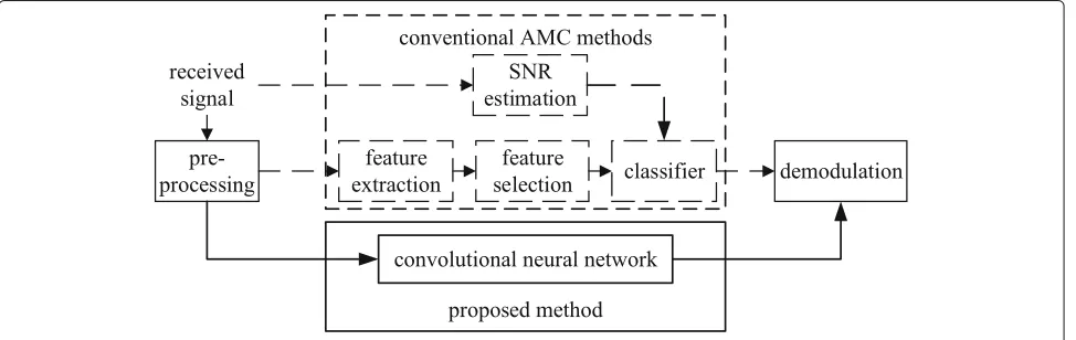
The AMC is an intermediate process that occurs between signal detection and demodulation at the receiver. The structure of our proposed AMC method in com-parison with the conventional ones is illustrated in Fig.1.

Preprocessing in Fig.1 refers to sampling and quanti-zation for IF signals. The procedures inside the dashed frame, which include the feature extraction, feature selec-tion, and classifier, are replaced by the CNN proposed here. The CNN is pre-trained offline with proper amount of samples before it is deployed. Furthermore, as long as the SNR range of the communication channel is known, the CNN can learn the features that adapt to the cor-responding condition. This property makes our method independent from the SNR estimation.

2.1 Signal model

In this paper, signals are processed in IF and are corrupted by AWGN. Then, the received signal can be denoted as

r(t)=s(t)+n(t), (1)

wheres(t) is the transmitted signal of different modula-tion types,n(t) is AWGN, and SNR is defined asPs/Pn

(Ps is the power of signal andPn is the power of noise).

The modulation set studied in this paper includesM-ASK, M-FSK,M-PSK (M = 2, 4, 8),M-QAM (M = 4, 16, 64), OFDM, MSK, and LFM. ForM-ASK,M-FSK, andM-PSK (M=2, 4, 8) signals,s(t)is expressed as

s(t)=Am

n

ang(t−nTs)cos[ 2π(fc+fm)t+ϕ0+ϕm] ,

(2)

where Am,an,Ts,fc,fm,ϕ0, and ϕm are the modulation

amplitude, symbol sequence, symbol period, carrier fre-quency at IF, modulation frefre-quency, initial phase, and

modulation phase, respectively, andg(t)is the gate func-tion represented as:

g(t)=

1 if 1tTs

0 other . (3)

ForM-QAM (M=4, 16, 64) signals, we have

s(t)=Am

n

ang(t−nTs)cos(2πfct+ϕ0)

+Am

n

bng(t−nTs)cos(2πfct+ϕ0)

, (4)

where an,bn ∈

2m−1−√M,m = 1, 2, ...,√M, and two carriers are modulated byanandbn, respectively.

The OFDM signal, which is the output of a multicarrier system, can be expressed as

s(t)=

n

(an+jbn)exp(j2πfnt)

=

n

ancos(2πfnt)−bnsin(2πfnt)

, (5)

whereanandbnare the in-phase component and

orthog-onal component of the symbol sequence on the n-th subcarrier, respectively, andfnis the frequency of then-th

subcarrier.

The LFM signals in a period are denoted as

s(t)=Amcos[ 2π(f0+kt)t] t∈

−Ts

2 ,

Ts

2 , (6)

where k andf0 are defined as the chirp rate and initial frequency, respectively.

Finally, for MSK signals, we have

s(t)=cos

2πfct+π

an(k)

2Ts +ϕk

(k−1)TstkTs

, (7)

where an(k) denotes the k-th symbol in the symbol

sequence, andϕkis the phase constant of thek-th symbol.

2.2 Convolutional neural network

CNNs are simply NNs that use convolution in place of general matrix multiplication in at least one of their layers [22]. Typical CNN architectures consist of three differ-ent types of layers: convolutional layer, pooling layer, and fully connected layer. There is an extra softmax regression layer deployed as the classifier at the last layer of the CNN in supervised learning. In this paper, we replace the fully connected layer with a global average pooling layer, so that there is no fully connected layer.

2.2.1 Convolutional layer

In convolutional layers, there are several convolution ker-nels (also known as filters) to process the received signal. Since the received signal is a 1-dimensional vector in AMC, the kernel is also a 1-dimensional vector. Suppose that thel-th layer of an NN is a convolutional layer,Ns,Lls,

N_kl, andLl_k represent the number of inputs, length of the input, number of kernels, and length of kernels of thel-th layer, respectively. The convolution operation [23] in the l-th layer is described as follows:

hl_k=f

xl×W_kl+bl_k

xl×W_kl(i)=

∞

a=−∞

x(a)W_kl(i−a),

(8)

wherex ∈RNs×Lsl _{is the set of inputs,W} ∈RNkl×L l k is the

set of kernels, andb∈RNs_{is the bias for each output. The}

output of thek-th

k=1, 2, ...,N_kl

kernel is denoted by

(8), andxl ×W_kl is the convolution betweenxl andW_kl. Assume that the length of the output isLl

o. The output

hl∈RNkl×Llo_{is the set of output, which is also known as the}

feature map.f(·)is the activation function to achieve the nonlinear mapping of outputs, which is often the sigmoid or tanh function. In this paper, the exponential linear unit (ELU) [24] is selected as the activation function, which is denoted as

f(x)=

x if x0

α(ex_{−1) if x<0}. (9)

The ELU is a simple piecewise function derived from the rectified linear unit (ReLU). It is designed to overcome gradient vanishing [25] while accelerating the convergence speed.

2.2.2 Max-pooling and global average pooling

The pooling layer is another important type of layer in the CNN. As mentioned, the convolutional layer performs several convolutions to produce a set of outputs, each of which runs through a nonlinear activation function (ELU). Then, a pooling function is used to further modify the out-put of the layer. A pooling function replaces the outout-put of the net at a certain location with a summary statistic of

the nearby outputs [23]. Max pooling is used in this paper, which is an operation that reports the maximum output within a pooling window [26]. Assume that the output of a convolutional layerhlis max-pooled. The outputhl+1is shown as

hl_k+1(i)=maxhl_kml+1(i−1)+1,hl_kml+1(i−1)+2,

...,hl_kml+1(i−1)+Lp

,

(10)

wherei

Ll_o−Ll_p+1

/ml+1+1,Ll_p+1is the length of the pooling window;ml+1is the margin between two adjacent pooling windows, which is also known as the stride.

Global average pooling [27] is applied after the last con-volutional layer. It takes the average of each feature map, and the output vector is directly fed into the softmax layer. Similarly, we assume that the output of the former convolutional layer is hl, which contains the output of N_kl kernels. The output of global average pooling hL_k is represented as

hL_k = 1

Ll

o Llo

i=1

hl_k(i), k=1, 2, ...,N_kl. (11)

2.2.3 Batch normalization

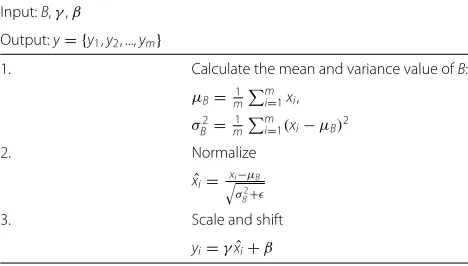
The batch normalization (BN) layer can accelerate deep network training by reducing the internal co-variate shift [28]. The internal covariate shift is defined as the change in distribution of output of each layer during train-ing. The changes are commonly caused by unbalanced nonlinear mapping (e.g., ELU activation). In stochas-tic gradient descent, a single mini-batch is represented as B = {x1,x2, ...,xm}, and the output yi is

normal-ized by the BN layer. Suppose that the mean and vari-ance of B are denoted as μB and σB, respectively.

The procedures of BN are shown in Table1.

In the BN process, parametersγ andβmust be learned with the training process of CNN. is a small quan-tity added to variance to avoid dividing by zero. BN is

Table 1Procedures of batch normalization

Input:B,γ,β

Output:y= {y1,y2, ...,ym}

1. Calculate the mean and variance value ofB:

μB= m1 m

i=1xi, σ2

B = m1 m

i=1(xi−μB)2

2. Normalize

ˆ

xi=xi−μB

σ2

B+

3. Scale and shift

deployed before the activation function when it is pro-posed, but experiments prove that BN should occur after the activation function [29]. As a result, BN is applied after each activation function in this paper.

2.2.4 Softmax regression

The last layer of the CNN in supervised learning is the softmax regression layer. Softmax regression is a multi-class multi-classifier generalized from logistic regression, whose output is a set of probability distributions of different classes. Considering ann-class classification problem, the input of the softmax regression ishL, which is the

out-put of the global average pooling layer, and the outout-put of softmax regressionyocan be denoted as:

P(yo=c|hL,WL,bL)=

exp(WLchL+bLc)

n

i=1exp(WLihL+bLi)

, (12)

wherec=1, 2, ...,n,WL,bLis the weight and bias between

the former output and the softmax. The neuron with the maximum output is selected as the classification result, which is also the output of the entire CNN. The loss func-tion of the CNN is defined asJ(W,b). Then, the training process is described as

arg min

W,bJ(W,b). (13)

The problem in (13) can be solved by a gradient descent. Partial derivatives are calculated using the back-propagation method [30] and used to updateW andb. The process is as follows:

W :=W−α∂J(W,b)

∂W

b:=b−α∂J(W,b)

∂b ,

(14)

whereαis known as the learning rate, which controls the update step of the parameters.

3 Numerical results and discussion 3.1 Simulation parameters

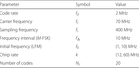
All signals are generated based on the description in Section2, and the parameters of modulation are shown in Table2. The number of subcarriers in the OFDM signal

Table 2Modulation parameters

Parameter Symbol Value

Code rate fd 2 MHz

Carrier frequency fc 70 MHz

Sampling frequency fs 400 MHz

Frequency interval (M-FSK) f 10 MHz

Initial frequency (LFM) f0 (1, 10) MHz

Chirp rate k (12, 60) MHz

Number of codes Nc 20

is set toNc, and the subcarriers are modulated by 4PSK.

Additionally, we denote the SNR of the training samples and the SNR of the testing samples as SNRtr and SNRte,

respectively.

The CNN that we built for AMC consists of 16 convolu-tional layers, whose structure is similar to that of VGG-19 [31] (as shown in Table 3). The input size of the CNN can be calculated byfs·Nc/fd = 4000. The parameters

of the convolutional layers and pooling layers in thel-th layer take the form of

N_kl,Ll_k

,

Ll_p,ml

, respectively. Sig-nals are normalized to [−1, 1] with zero mean and are then processed by CNN. The CNN in this paper is imple-mented by the DL library, Keras [32], with Theano [33] as its backend.

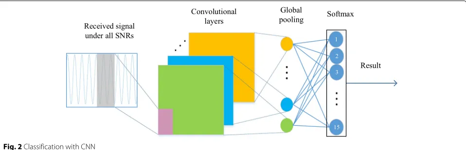
3.2 Classification with CNN

In this section, signals are directly classified by CNN, and the results are from the final softmax layer. The process is displayed in Fig. 2. The classification accuracy under fixed SNR level is firstly displayed in Table4for SNRte= SNRtr. We generate 20000 training samples and 1000 test-ing samples for each modulation type at every SNR level. As observed from Table 4, the classification accuracy is 90% when SNRtr = −10 dB. This finding demonstrates excellent performance for AMC methods. The classifica-tion accuracy of all individual classes reaches almost 100% when SNRtr 5 dB. Because our channel is AWGN, the signals with amplitude modulation suffer most from the decreasing SNRtr. The accuracy of 4ASK and 8ASK dra-matically deteriorates when SNRtr 0 dB. Only 48.8% of 4ASK are correctly classified under−10 dB. The accu-racy of 16QAM and 64QAM also rapidly decreases when SNRtr−4 dB.

The detailed classification result when SNRtr= −10 dB is shown in Table 5. Signals with identical classes but different orders (e.g., 2ASK, 4ASK, and 8ASK) may be mixed, but there is very little interclass misclassification. For example, nearly half of 4ASK signals are classified as 2ASK and 8ASK, but all of them areM-ASK signals. The intraclass classification result for M-QAM and M -ASK signals may be unsatisfactory, whereas the interclass accuracy remains nearly 100%.

Table 3Structure of CNN

Layer number Layer type Parameters Layer number Layer type Parameters

1 Conv (35, 4) 12 Conv (50, 4)

2 Convl (35, 4) 13 Conv (50, 4)

3 Pooling (2, 2) 14 Conv (50, 4)

4 Conv (40, 4) 15 Conv (50, 4)

5 Conv (40, 4) 16 Pooling (2, 2)

6 Pooling (2, 2) 17 Conv (60, 4)

7 Conv (45, 4) 18 Conv (60, 4)

8 Conv (45, 4) 19 Conv (60, 4)

9 Conv (45, 4) 20 Conv (60, 4)

10 Conv (45, 4) 21 Global pooling None

11 Pooling (2, 2) 22 Softmax 15

The above results are obtained under the assump-tion of SNRte = SNRtr. However, SNRtr (commonly obtained from SNR estimation) is often inaccurate in practice. Moreover, SNRte should be the actual channel SNR, which may also be unstable or rapidly varying under certain conditions (e.g., satellite communication). To study this problem, the CNN is trained under a cer-tain SNR range to make the trained CNN robust to SNR variations. In this case, the training SNR is denoted as SNRtr ∈[ SNRmintr , SNRmaxtr ] and separately takes values of [−10, 0] dB, [−5, 15] dB, and [ 0, 20] dB. The line of classification accuracy when SNRtr=SNRteis plotted for comparison. The results are shown in Fig.4.

The CNNs trained in a certain SNR range are robust to SNR variations when SNRteis in the range of SNRtr. The classification accuracy is also notably close to that under SNRte = SNRtr. The generalization ability can stretch to the higher SNR range when SNRteis not in the range of SNRtr. For CNN trained under [−10, 0] dB, the classification accuracy can still reach 96% under 20 dB. The CNNs can be robust to SNR variation; thus, they can be deployed in a certain SNR range.

3.3 Feature learning with CNN

For most existing DL-based AMC methods, DL networks are treated as classifiers. However, DL networks also have the powerful capability of feature learning. Only the last layer of a CNN (softmax layer) is a classifier; thus, the input of softmax layerhLis equal to the features learned by

the CNN. Thus, we can analyze these features by observ-inghL(the output of the global average pooling layer). The

multi-dimensional scaling (MDS) method [34] is applied to maphL, which is a 60-dimensional vector, into a 2-D

axis for convenient observation. Features under SNRtr = −10 dB and SNRtr =5 dB are normalized and visualized in Fig.5.

The features of 4PSK and 8PSK signals are completely mixed in Fig. 5a, which also shows why these two cat-egories are poorly classified when SNRtr = −10 dB. The situation is similar to 4ASK and 8ASK signals. In contrast to Fig.5a, the distribution of CNN-learned fea-tures in Fig.5b is much better because of the increase in SNR. Most signals in the same categories are distributed in the same cluster, and the margins among different clusters are evident, which implies that the extracted

Fig. 3The classification accuracy of CNNs with different number of layers versus SNR

tures are well suited for classification. The cluster of LFM signals consists of several small clusters because parts of the modulation parameters of LFM signals are randomly generated.

We obtain several CNNs that are robust to SNR vari-ations by training them in a certain SNR range as in the previous subsection. We can learn noise-robust features in a notably similar manner. The dimension reduction to hLis accomplished using the neural networks by adding a

hidden layer containing four neurons between the global average pooling layer and softmax layer (see Fig.6). Thus, the learned features will be 4-dimensional vectors. Each

dimension of the feature under different SNR levels is separately plotted (SNRtr ∈[−5, 15] dB) in Fig.7, where feature 1, feature 2, feature 3, and feature 4 correspond to the output of the four neurons. We can find that for each modulation type, at least one feature rarely changes with the SNR (e.g., feature 1 and feature 4 of 2ASK and feature 2 of OFDM and 4PSK). These features are robust to SNR variation; thus, they are expected to provide an excellent generalization ability under the varying SNRte.

A linear support vector machine (SVM) is deployed to test the generalization ability of the learned features. Unlike the previous subsection, the SVM is trained for a

a

b

Fig. 5Distribution of learned features under SNRtr= −10 dB and SNRtr=5 dB (visualized by MDS).aDistribution of CNN-learned features (SNRtr= −10 dB).bDistribution of CNN-learned features (SNRtr=5 dB)

fixed SNR level. In this case, SNRtr takes the values of −5, 0, 5, 10, 15 dB in turn, and the classification accuracy is tested for [−10, 20] dB. The results are illustrated in Fig.8.

The classification accuracies of all SVMs are notably similar. The SVM trained for −5 dB performs slightly worse than the others because the values of the learned features fluctuate the most for [−5, 0] dB, and most of them are stable when SNRtr 0 dB (see Fig. 7). The generalization ability of CNN-learned features is

outstanding. The SVM trained for −5 dB can correctly classify 99.1% of signals under 20 dB, and the classification accuracy of signals for−5 dB is 90% for the SVM trained for 15 dB. In this way, the classifiers trained by CNN-learned features can reduce their dependency on the SNR estimation.

Fig. 6Feature learning with CNN

and CNN is deployed to extract features under [0, 20] dB. Then, a linear SVM is deployed to evaluate the perfor-mance of our method. SNRtr takes the values of 0, 10, 20 dB in turn and classification accuracy is tested for [0, 20] dB. From the result in Fig.9, we can observe that the performance is significantly improved, especially under low SNRs, indicating the superiority of CNN-learned features.

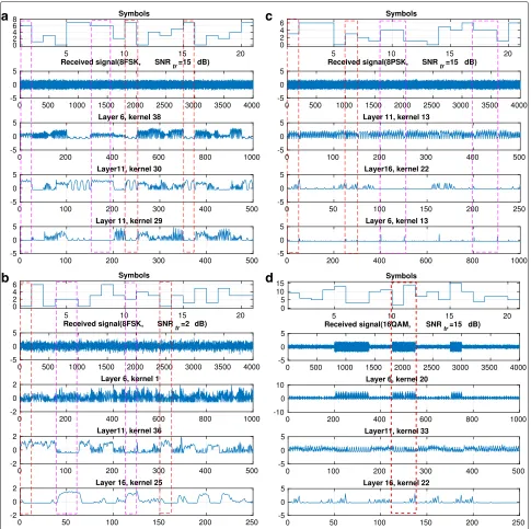
3.4 Visualization of feature learning process

We have proven that the CNN can learn efficient features for classification. In this section, the process of feature learning by CNN is analyzed by visualizing the outputs of the intermediate layers. The signals modulated by the same symbols are in the dashed box with identical colors. We select some typical outputs of intermediate layers and plot them in Fig.10. For 8FSK signals in Fig.10a, identical

a

b

c

d

Fig. 8Classification accuracy of SVM trained using the CNN-learned features

symbols correspond to identical modulation frequencies. Each convolution kernel retains only a portion of the fre-quency components. The frefre-quency component of sym-bol 6 (in the magenta box) is maintained in the 38th kernel of layer 6 but filtered out in the 29th kernel of layer 11, e.g., each kernel concerns only a part of the information from the received signals. By comparing Fig.10a with Fig.10b, we also find that feature learning becomes harder with the decrease in SNRtr. Different frequencies can be

eas-ily distinguished in layer 6 when SNRtr = 15 dB, but the differences are not obvious when SNRtr = 2 dB. Hence, we need more layers when the SNR is low.

Similar to the frequency information in Fig. 10a, the kernel can also learn the phase information in Fig. 10c. For the 16QAM signal in Fig. 10d, the amplitude infor-mation and phase inforinfor-mation are recorded by the 20th kernel of layer 6 and the 33rd kernel in layer 11, respectively. Thus, symbols 1 and 14, which are

a

b

c

d

Fig. 10Visualization of the outputs of intermediate layers.aSignal type=8FSK, SNRtr=15 dB.bSignal type=8FSK, SNRtr=2 dB.cSignal type= 8PSK, SNRtr=15 dB.dSignal type=16QAM, SNRtr=15 dB

ulated with identical amplitudes but different phases, can be distinguished through a combination of different kernels.

4 Conclusion

In this paper, an AMC method based on a CNN has been proposed. First, we have used the CNN as a powerful classifier. In total, 15 different modulation types have been studied, and the classification for fixed SNR and

Then, the features that the CNN learns from the received signals have been analyzed. Features are mapped to a 2-D axis using MDS, where we observe that most sig-nals in the same categories are distributed in the same cluster. The margins among different clusters are also evi-dent; thus, they are well suited for classification. Robust features learned under [−5, 15] dB are also studied. Robust features are insensitive to the SNR variation, so they have strong generalization ability. The SVM trained by these robust features under−5 dB can correctly clas-sify 99.1% of signals when the testing SNR is 20 dB. As a result, CNNs trained in this way can be robust to SNR variation.

Additionally, we visualize some typical outputs of the intermediate layers. We find that each kernel in the con-volutional layer can learn different information from the received signal. The information includes the phase, fre-quency, amplitude, and other information that is difficult for us to understand.

Abbreviations

AMC: Automatic modulation classification; AWGN: Additive white Gaussian noise; CNN: Convolutional neural network; DL: Deep learning; ELU: Exponential linear unit; FB: Feature based; HOC: High-order cumulant; IF: Intermediate frequency; LB: Likelihood based; ReLU: Rectified linear unit; SCF: Spectral correlation function; SNR: Signal to noise ratio; SVM: Support vector machine

Funding

The research in this article is supported by “the National Natural Science Foundation of China” (Grant nos. 61571167, 61471142, 61102084 and 61601145)

Availability of data and materials

The datasets used during the current study are available from the corresponding author on reasonable request.

Authors’ contributions

SZ proposed the framework of the whole algorithm. ZYin handled all the simulations. ZW made full contribution in the acquisition of funding. YC was a major contributor in writing the manuscript. NZ made all the figures and tables in the manuscript. ZYang made the visualization in the last section. All authors read and approved the final manuscript.

Competing interests

The authors declare that they have no competing interests.

Publisher’s Note

Springer Nature remains neutral with regard to jurisdictional claims in published maps and institutional affiliations.

Author details

1_{School of Electronics and Information Engineering, Harbin Institute of}

Technology, No. 92 West Dazhi Street, Nangang District, Harbin, China. 2_{School of Engineering, University of Warwick, Coventry CV4 7AL, UK.}3_School

of Information and Communication Engineering, Dalian University of Technology, No.2 Linggong Road, Ganjingzi District, Dalian, China.

Received: 17 October 2018 Accepted: 4 March 2019

References

1. J. L. Xu, W. Su, M. Zhou, IEEE Trans. Syst. Man Cybernet. Part C Appl. Rev.

41(4), 455–469 (2011)

2. A. Hazza, M. Shoaib, S. A. Alshebeili, A. Fahad, inCommunications, Signal Processing, and Their Applications (ICCSPA), 2013 1st International Conference On. An overview of feature-based methods for digital modulation classification (IEEE, 2013), pp. 1–6.https://ieeexplore.ieee.org/abstract/ document/6487244

3. E. E. Azzouz, A. K. Nandi, Automatic identification of digital modulation types. Signal Process.47(1), 55–69 (1995)

4. J. J. Popoola, R. van Olst, A novel modulation-sensing method. IEEE Veh. Technol. Mag.6(3), 60–69 (2011)

5. J. Liu, Q. Luo, inCommunication Technology (ICCT), 2012 IEEE 14th International Conference On. A novel modulation classification algorithm based on daubechies5 wavelet and fractional fourier transform in cognitive radio (IEEE, 2012), pp. 115–120.https://ieeexplore.ieee.org/ abstract/document/6511199

6. Y. Lv, Y. Liu, F. Liu, J. Gao, K. Liu, G. Xie, inComputer and Information Technology (CIT), 2014 IEEE International Conference On. Automatic modulation recognition of digital signals using CWT based on optimal scales (IEEE, 2014), pp. 430–434.https://ieeexplore.ieee.org/abstract/ document/6984692

7. D. Das, A. Anand, P. K. Bora, R. Bhattacharjee, inSignal Processing and Communications (SPCOM), 2016 International Conference On. Cumulant based automatic modulation classification of QPSK, OQPSK,π/4-QPSK and 8-PSK in MIMO environment (IEEE, 2016), pp. 1–5.https://ieeexplore. ieee.org/abstract/document/7439996

8. A. Hazza, M. Shoaib, A. Saleh, A. Fahd, Robustness of digitally modulated signal features against variation in HF noise model. EURASIP J. Wirel. Commun. Netw.2011(1), 24 (2011)

9. U. Satija, M. Manikandan, B. Ramkumar, inIndustrial and Information Systems (ICIIS), 2014 9th International Conference On. Performance study of cyclostationary based digital modulation classification schemes (IEEE, 2014), pp. 1–5.https://ieeexplore.ieee.org/abstract/document/7036609 10. P. M. Rodriguez, Z. Fernandez, R. Torrego, A. Lizeaga, M. Mendicute, I. Val,

Low-complexity cyclostationary-based modulation classifying algorithm. AEU Int. J. Electron. Commun.74, 176–182 (2017)

11. M. W. Aslam, Z. Zhu, A. K. Nandi, Automatic modulation classification using combination of genetic programming and KNN. IEEE Trans. Wirel. Commun.11(8), 2742–2750 (2012)

12. K. Hassan, I. Dayoub, W. Hamouda, M. Berbineau, inIntelligent Transport Systems Telecommunications,(ITST), 2009 9th International Conference On. Automatic modulation recognition using wavelet transform and neural network (IEEE, 2009), pp. 234–238.https://ieeexplore.ieee.org/abstract/ document/5399351

13. V. Orlic, M. Dukic, Multipath channel estimation algorithm for automatic modulation classification using sixth-order cumulants. Electron. Lett.

46(19), 1348–1349 (2010)

14. C. Szegedy, W. Liu, Y. Jia, P. Sermanet, S. Reed, D. Anguelov, D. Erhan, V. Vanhoucke, A. Rabinovich, inProceedings of the IEEE conference on computer vision and pattern recognition. Going deeper with convolutions, (2015), pp. 1–9. https://www.cv-foundation.org/openaccess/content_cvpr_2015/html/ Szegedy_Going_Deeper_With_2015_CVPR_paper.html

15. Y. Wu, M. Schuster, Z. Chen, Q. V. Le, M. Norouzi, W. Macherey, M. Krikun, Y. Cao, Q. Gao, K. Macherey, et al., Google’s neural machine translation system: bridging the gap between human and machine translation. arXiv preprint arXiv:1609.08144 (2016)

16. G. J. Mendis, J. Wei, A. Madanayake, inCommunication Systems (ICCS), 2016 IEEE International Conference On. Deep learning-based automated modulation classification for cognitive radio (IEEE, 2016), pp. 1–6.https:// ieeexplore.ieee.org/abstract/document/7833571/

17. A. Dai, H. Zhang, H. Sun, inSignal Processing (ICSP), 2016 IEEE 13th International Conference On. Automatic modulation classification using stacked sparse auto-encoders (IEEE, 2016), pp. 248–252.https:// ieeexplore.ieee.org/abstract/document/7877834

18. T. J. O’Shea, J. Corgan, T. C. Clancy, inInternational Conference on Engineering Applications of Neural Networks. Convolutional radio modulation recognition networks (Springer, 2016), pp. 213–226.https:// link.springer.com/chapter/10.1007/978-3-319-44188-7_16

19. J. Fu, C. Zhao, B. Li, X. Peng, inThe Proceedings of the Third International Conference on Communications, Signal Processing, and Systems. Deep learning based digital signal modulation recognition (Springer, 2015), pp. 955–964. https://link.springer.com/chapter/10.1007/978-3-319-08991-1_100

21. D. Zhang, W. Ding, B. Zhang, C. Xie, H. Li, C. Liu, J. Han, Automatic modulation classification based on deep learning for unmanned aerial vehicles. Sensors.18(3), 924 (2018)

22. Y. LeCun, et al., inConnectionism in perspective. Generalization and network design strategies, vol. 19 (Citeseer, 1989)

23. I. Goodfellow, Y. Bengio, A. Courville,Deep learning. (MIT Press, 2016) 24. D.-A. Clevert, T. Unterthiner, S. Hochreiter, Fast and accurate deep

network learning by exponential linear units (elus). arXiv preprint arXiv:1511.07289 (2015)

25. S. Hochreiter, The vanishing gradient problem during learning recurrent neural nets and problem solutions. Int. J. Uncertain. Fuzziness Knowl.-Based Syst.6(02), 107–116 (1998)

26. K. Jarrett, K. Kavukcuoglu, Y. LeCun, et al., inComputer Vision, 2009 IEEE 12th International Conference On. What is the best multi-stage architecture for object recognition? (IEEE, 2009), pp. 2146–2153.https://www. computer.org/csdl/proceedings/iccv/2009/4420/00/05459469-abs.html 27. M. Lin, Q. Chen, S. Yan, Network in network. arXiv preprint arXiv:1312.4400

(2013)

28. S. Ioffe, C. Szegedy, Batch normalization: accelerating deep network training by reducing internal covariate shift. arXiv preprint arXiv:1502.03167 (2015)

29. D. Mishkin, N. Sergievskiy, J. Matas, Systematic evaluation of CNN advances on the ImageNet. ArXiv e-prints 1606.02228 (2016)

30. Y. Bengio, et al., Learning deep architectures for AI. Found. Trends® Mach. Learn.2(1), 1–127 (2009)

31. K. Simonyan, A. Zisserman, Very deep convolutional networks for large-scale image recognition. arXiv preprint arXiv:1409.1556 (2014) 32. F. Chollet, et al., Keras. GitHub (2015).https://keras.io/getting-started/

faq/#how-should-i-cite-keras

33. R. Al-Rfou, G. Alain, A. Almahairi, C. Angermueller, D. Bahdanau, N. Ballas, F. Bastien, J. Bayer, A. Belikov, A. Belopolsky, et al., Theano: A python framework for fast computation of mathematical expressions. arXiv preprint arXiv:1605.02688 (2016)

34. A. Buja, D. F. Swayne, M. L. Littman, N. Dean, H. Hofmann, L. Chen, Data visualization with multidimensional scaling. J. Comput. Graph. Stat.17(2), 444–472 (2008)