Revisiting exact kNN query processing with probabilistic data space transformations

warwick.ac.uk/lib-publications

Manuscript version: Author’s Accepted Manuscript

The version presented in WRAP is the author’s accepted manuscript and may differ from the

published version or Version of Record.

Persistent WRAP URL:

http://wrap.warwick.ac.uk/112261

How to cite:

Please refer to published version for the most recent bibliographic citation information.

If a published version is known of, the repository item page linked to above, will contain

details on accessing it.

Copyright and reuse:

The Warwick Research Archive Portal (WRAP) makes this work by researchers of the

University of Warwick available open access under the following conditions.

Copyright © and all moral rights to the version of the paper presented here belong to the

individual author(s) and/or other copyright owners. To the extent reasonable and

practicable the material made available in WRAP has been checked for eligibility before

being made available.

Copies of full items can be used for personal research or study, educational, or not-for-profit

purposes without prior permission or charge. Provided that the authors, title and full

bibliographic details are credited, a hyperlink and/or URL is given for the original metadata

page and the content is not changed in any way.

Publisher’s statement:

Please refer to the repository item page, publisher’s statement section, for further

information.

Revisiting Exact

k

NN Query Processing with

Probabilistic Data Space Transformations

Atoshum Cahsai

, Christos Anagnostopoulos

, Nikos Ntarmos

, Peter Triantafillou

∗_{School of Computing Science, University of Glasgow, UK}

Email: [email protected],{christos.anagnostopoulos, nikos.ntarmos}@glasgow.ac.uk

†_{Department of Computer Science, University of Warwick, UK}

Email: [email protected]

Abstract—The state-of-the-art approaches for scalable kNN query processing utilise big data parallel/distributed platforms (e.g., Hadoop and Spark) and storage engines (e.g, HDFS, NoSQL, etc.), upon which they build (tree based) indexing methods for effi-cient query processing. However, as data sizes continue to increase (nowadays it is not uncommon to reach several Petabytes), the storage cost of tree-based index structures becomes exceptionally high. In this work, we propose a novel perspective to organise multivariate (mv) datasets. The main novel idea relies on data space probabilistic transformations and derives a Space Transfor-mation Organisation Structure (STOS) for mv data organisation. STOS facilitates query processing as if underlying datasets were uniformly distributed. This approach bears significant advan-tages. First, STOS enjoys a minute memory footprint that is many orders of magnitude smaller than indexes in related work. Second, the required memory, unlike related work, increases very slowly with dataset size and, thus, enjoys significantly higher scalability. Third, the STOS structure is relatively efficient to compute, outperforming traditional index building times. The new approach comes bundled with a distributed coordinator-based query processing method so that, overall, lower query processing times are achieved compared to the state-of-the-art index-based methods. We conducted extensive experimentation with real and synthetic datasets of different sizes to substantiate and quantify the performance advantages of our proposal.

I. INTRODUCTION ANDRELATEDWORK

In the era of big data, many devices continuously generate huge amounts of data, rendering traditional off-the-shelf data processing tools inadequate to cope with the ever growing data. To this end, several parallel/distributed processing approaches and systems have emerged, e.g., Hadoop-MapReduce [13] and Spark [40], but such frameworks cannot efficiently process some fundamental queries such as kNN.

For efficient exact kNN queries processing (N.B. in this paper we are not dealing with approximated kNN queries) several solutions are proposed: for e.g. MapReduce based [9], [1], [3], [16]; Spark based [39], [4], [38], [37]; and HBase based [7], [21], [22], [27]. But to save space, the current state of the art methods: the best from MapReduce echo system SHadoop [16], the best from Spark echo system Simba [37], and the best from HBase COWI/CONI [7] will be discussed; all these approaches deal with 2- or 3-dimensional data.

Both SHadoop and Simba maintain relatively large data-blocks, based on the block size of the Distributed File System (DFS) in which they operate; e.g., 128 MB in the case of the Hadoop DFS (HDFS). DuringkNN query processing, as each

block stores millions of data points, accessing such large data blocks incurs high disk and network I/O overheads.

To circumvent the issues faced by Simba and SHadoop, CONI/COWI divides a dataset into much smaller chunks a.k.a cells and stores the cells in NoSQL key-value datastore (HBase [19]). CONI/COWI surgically accesses only a very small but relevant number of data points and as such achieves up to three orders of magnitude lower query processing times comparing against Simba and SHadoop.

A dataset can be partitioned by a tree-based multivariate (mv) index approach such as Quad-Trees (QT) [17], R-Trees [20] and K-D trees [6]. During indexing process, those meth-ods build a tree-like data structure that assumed to reside in memory to serve as index. But when indexing a large-scale dataset, the size (in bytes) of the index can be quite large, and sometimes even surpassing the size of the dataset itself[35]. This is further aggravated when opting to divide a dataset into smaller cells.

To prevent the size of the index from exceeding the available memory, one can impose a lower limit on the cell size, and hence decreases the size of the tree. But for large-scale datasets, having large sized cells decreases performance and indeed the scalability of the approach. To alleviate this problem, CONI used a coordinator-based approach, storing part of the index in a key-value store (HBase); by doing this, CONI can have smaller cells without worrying about the index size. However, this approach has two drawbacks: (i) accessing HBase at query time incurs high disk I/O compared to an index that resides in memory, and (ii) CONI needs to replicate parts of the index contents in order to create a balanced tree and, as such, may have a larger disk footprint.

work well with non-uniformly distributed data [32], [7].

COWI/CONI partition a datset using a QuadTree (QT) in MapReduce, but a recent survey [32] that evaluates MapRe-duce based data partitioning methods concluded that even though QT provides better data proximity, efficiency for search queries, and low network transfer overhead as compared to other data partitioning methods, QT requires high index storage space, index building time, and has poor applicability in high dimensions. Also, the authors of SHadoop in [15] ran extensive experiments and measured data partitioning time of mv index approaches in MR. The main conclusion is that index building times of these mv index methods are very similar as the indexing process is dominated by the MR job that scans the whole file; the main difference between all those methods is the in-memory step which operates on a small sample, and this opens the space to incorporate more complicated techniques.

Therefore, the central conclusion is that current scal-able kNN query processing strategies suffer from significant drawbacks, especially for non-uniformly distributed datasets. Specifically, all related works: (1) fail to address the obvious efficiency and scalability problems that result from increasing index sizes; (2) struggle to index non-uniform big data; and/or (3) face problems related to high indexing time, high index storage space and poor applicability in higher dimensions. Fundamentally, keeping in mind that datasets can be massive and that any system would be called upon to execute a large number of different query types (not just kNN queries), the luxury ofkNN query processing using large indexes that grow with a size of a dataset is simply not affordable.

In this paper, we propose a novel perspective for organising datasets that alleviates the need for traditional mv indexes; our contributions stem from the following key observations:

First, Uniform Grid-based method performs exceptionally well over datasets that have a uniform distribution. This is due to the facts that: (i) as all cells have equal size, it enjoys good storage load balance; (ii) as all cells have equal width, all that is required to locate the cell to which a point belongs is the width of the cell and no any memory-hungry index; (iii) as its memory footprint is small and doesn’t grow with the size of the dataset and/or the number of cells, the domain space can be divided into small-sized cells thus benefiting query performance without adverse effects on index size and/or fault tolerance; and (iv) it has good applicability in high dimensions.

Second, unfortunately, real-world datasets rarely are uni-formly distributed. Furthermore, methods based on a uniform grid partitioning are not suitable for non-uniform datasets, as in those cases the distribution of points to cells can be very skewed, resulting in unpredictable and long query processing times when retrieving and processing large cells.

Third, when the Random Variables (RVs) of a dataset are independent, the distribution of the dataset can be transformed to joint uniform distribution. This can be achieved using well-known statistical methods, coined Independence Copula [18]. Even when the RVs are not independent, if the joint and marginal distributions of the RVs belong to the family of elliptical distributions [8], then removing correlation between the RVs implies independence [29].

Fourth, however, many real world datasets are generated by

non elliptical mv distributions; therefore, removing correlation between RVs of such datasets does not imply independence. Fortunately, any continuous distribution can be approximated by finite Gaussian Mixture Models (GMMs) to arbitrary accuracy [26]. Clustering a dataset with the right number of components enables GMMs to approximate the unknown underlying probability density function of a dataset [26]. Since each component (cluster) of a GMM has a mv Gaussian (and thus elliptical) distribution, removing the correlation between RVs of each component transforms the RVs of the cluster to

independent RVs. Therefore, using the Independence Copula method, the distribution of each component can be transformed to a joint uniform distribution.

In this paper, following the above observations, we exploit the fact that typically the input dataset is either generated by a family of elliptical distributions or can be approximated well by GMM. The central idea of our work is that, by transforming the data generated or approximated by a family of elliptical distributions into uniformly distributed data, we are able to build a grid index (with a uniformly distributed grid cell population) over the dataset. As a result, traditional (tree-like) indexes are not needed, in memory or on disk, and thus we can avoid sacrifices to performance and scalability.

Contribution:Our salient contributions are:

• A novel approach for organising mv datasets, based on a Space Transformation Organisation Structure (STOS), which facilitates kNN query processing as if the under-lying datasets are uniformly distributed. This approach ensures:

◦ Extremely low memory footprint, several orders of magnitude smaller than index-based approaches. ◦ A memory footprint that is practically independent of

the dataset size and the number of data points per grid cell – a fact that ensures scalability.

◦ Fast STOS computation time, that is smaller than traditional index building times, by several orders of magnitude.

◦ Easy and fast recoverability, as the minute size of STOS allows for several copies of it to be distributed, thus allowing the system to be up and running quickly after failures.

◦ Query processing similar or better than traditional (tree-based) indexing approaches.

The rest of the paper is organised as follows: § II-A presents definitions, while § II-A elaborates on the problem analysis and fundamentals. Then, §II-A explains the prelimi-nary, §III details our proposed method,§IV and§V reports on implementation details and experimental evaluation, while §VI concludes the paper.

II. DATASPACETRANSFORMATIONFUNDAMENTALS

A. Core Definitions

Definition 1. If the total number of data points in a uniformly distributed domain space is|D|, andαnumber of data points are needed to be stored per cell, the domain space can be partitioned into|C|=|D|/αequal-width cells. The cell width

Fig. 1. Original Distribution Fig. 2. Marginally uniform

Definition 2. Let a closed interval on a number line start at 0 and be divided into finite consecutive half-open intervals, each of which has equal lengthr. Given a random real number

q≥0, the starting point of the half-open interval in which it lies can be computed bybq_rc ·r.

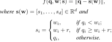
Definition 3 ([30]). The minimum distance between a mv query point q and a Minimum Bounding hyper-Rectangle (MBR)b is denoted by the Euclidean norm:

f(q,w;s) =kq−s(w)k,

where s(w) = [s1, . . . , sd]∈Rd and

si=

 



wi, ifqi< wi;

wi+r, ifqi≥wi+r;

qi, otherwise.

wherer isb’s width andw its lower-left coordinates.

By transforming the arbitrary distribution of a dataset into multivariate (mv) joint uniform distribution, one can utilise a uniform grid to gain the advantages mentioned previously. In the remainder of this section, we explain how to transform an arbitrary mv distribution into mv joint uniform distribution, which is the core idea behind the new proposed approach.

B. Statistical Analysis via Copulas

Copulas are mv probability distributions for which the marginal probability distribution of each variable is uniform, and are used to describe dependence between random variables (RVs). According to Sklar’s theorem (Theorem 1), any mv distribution can be written in terms of a univariate uniform distribution of each RV and a copula that captures the depen-dence among those RVs.

Theorem 1. (Sklar’s theorem [33]). Let H be a d-dim. cumulative distribution function H(x1, x2, . . . , xd) =

P[X1≤x1, X2≤x2, . . ., Xd≤xd] of random variables

(X1, X2, . . . , Xd) with marginals Fi(x) =P[Xi≤xi].

Then there exists a copula distribution C with uniform marginals such that H(x1, x2, . . . , xd) =

C(F1(x1), F2(x2), . . . , Fd(xd)).

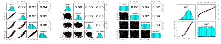
Example 1:Consider the real dataset called The Population Biology of Abalone – Haliotis species – in Tasmania [25]

(hereinafter referred to as simply Abalone). Abalone has eight RVs, but to save space four RVs are shown in a scatterplot matrix in Figure 1. The bivariate joint distributions of those RVs are shown in the lower diagonal, the upper off-diagonal shows the Pearson correlation, and the entries on the diagonal depict the marginal distribution of each RV. The four

RVs of Abalone are expressed by copulas as shown in Figure

2. It is worth noting that the bivariate distribution between any two of RVs of Figure 2 is not necessarily uniform.

In the literature, there are several families of copulas. Here, we focus only on a specific type of copula called Independence copula whose RVs are statistically independent of each other. The marginal and joint distribution of Independence copula is uniform. However, since the RVs of most real-world datasets have some kind of dependence, Independence Copula cannot be directly applied in these cases. On the other hand, two independent RVs have zero correlation, but the inverse is not always true. Nonetheless, when the marginal and joint distribu-tions of RVs of a dataset are elliptical distribudistribu-tions, removing correlation results in independent RVs [29]. Unfortunately, many real-world datasets have non-elliptical distributions, so removing the correlations among RVs of such datasets does not yield independent RVs. Any continuous mv distribution can be approximated arbitrarily well by finite Gaussian Mixture Models (GMM) to arbitrary accuracy [26]. A mv Gaussian distribution is a member of elliptical distributions thus by removing the correlation among RVs that belong to a GMM, it eliminates the dependencies among them.

We can transform any arbitrary distribution of a dataset to have a joint uniform distribution in the following four steps: (i)clustering: approximate the distribution of the dataset using GMM. Then, within each GMM cluster: (ii)de-correlation: re-move statistical correlation among RVs; (iii)marginal uniform transformation: transform the marginal distribution of every RV to standard uniform distribution; (iv)goodness of fit testing: check if every pair of RVs can be defined by an independence copula. Our approach elaborates on these steps.

C. Data Clustering Methodology

Gaussian Mixture Models (GMM) are used for clustering data points that are heterogeneous and stem from different sources. GMM models the density of mv RVs as a weighted sum of Gaussian density and is defined as:

f(x) = ΣM_m=1πmψm(x;µm,Σm) (1)

wherex is a RV,ψm(x;µm,Σm)is a Gaussian density with mean vector µ_m and covariance matrix Σm, and πm are the positive mixing weights that satisfy the constraintΣM

m1πm= 1.

Given M is the smallest integer such that πm > 0 for 1 ≤

m ≤M, and (µa,Σa)6= (µb,Σb) for 1≤a6=b≤M, the complete set of parameters of GMM θ ={µ₁,Σ1, . . . ,µm,

ΣM, π1, . . . , πM} can be estimated by maximum likelihood

method via the EM algorithm[14].

Fig. 3. Original Data Space Fig. 4. Independent Data Space Fig. 5. Uniform Data Space Fig. 6. PDF and ECDF

D. Removing Statistical Correlation

After clustering a dataset, we can remove the correlation between RVs of a cluster to transform the RVs into independent RVs. We therefore explain how to remove dependency between the RVs and then describe how to transform the marginal distribution of each RVs to a standard uniform. The correlation between RVs of a vector x such that x∈ Mi, where Mi is

the ith cluster of a GMM, can be removed by multiplying x

by awhitening matrixA:

Σ−1=ATA, (2)

where Σ−1 is the inverse of the covariance matrix of Mi.

Usually, Cholesky decomposition is adopted to estimate matrix

A fromΣ−1.

Example 2:Using GMM, after clustering the four RVs of dataset Abalone into two components, the scatter plot matrix of one of the components is reported in Figure3. As shown in the upper off-diagonal of the figure, there is a strong correlation between the RVs of the cluster. After multiplying by the whitening matrix A, the correlation between RVs becomes zero, as can be seen at the upper off-diagonal plots in Figure

4. This implies that the original RVs of the GMM cluster are transformed into independent RVs.

E. Transforming to Uniform Data Space

To transform the marginal distributions of the independent RVs to standard uniform, the well known Probability Integral Transformation (PIT) Theorem 2 is applied.

Theorem 2. (Probability Integral Transformation [10, chapter 2, p. 54]). Let random variable Y have a continuous distri-bution with cumulative distridistri-bution function (cdf) FY(y) =

P(Y ≤y)and define the random variableU =FY(y). Then

U is uniformly distributed in (0,1) withP(U ≤u) =u,0 <

u <1.

Proof: ( see [10, chapter 2, p. 54])

By convention, a RV Y generated by a continuous prob-ability distribution function (pdf) is denoted byp(y)and the cumulative distribution function of Y is denoted by FY(y). The relationship between p(y) and FY(y) of a RV Y is: if

R+∞

−∞ p(y)dy= 1, then there exists another continuous random variable u= FY(y) = R

y

−∞p(y)dy =P(Y ≤ y), thus u is called acdf ofy, and as suchUis a monotonic non-decreasing function of Y where 0 < u < 1. To compute the cdf of a RV Y requires to solve FY(y) =

Ry

−∞p(y)dy, but for many distributions the integral is not available in a closed form. Hence, the cdf of such RVs can be computed empirically:

ˆ

FY(y) =

1

nΣ

n

i=11xi≤y (3)

where xi is the ith data point in the dataset, n is the total number of data points in the dataset and1xi ≤y= 1 ifxi≤y

otherwise ₁xi≤y= 0.

Example 3: Consider one of the RVs of the previous example, called Length. To compute theecdfof the Length RV, allnLength values in the dataset must be sorted in ascending order (assuming there are n in points the Abalone dataset). Then starting from zero, and by jumping1/nfor each of then

data points, a monotonic increasing function is drawn between 0 and 1; see the upper right and the lower left of Figure 6. The upper left histogram of figure 6 shows the marginalpdf of Length; whereas the lower right histogram shows the marginal

cdf of Length. NB: the cdf of a continuous RV follows the standard uniform distribution.

For the sake of completeness, we provide (3) to expresscdf

of a RV has uniform distribution. However, computingcdf in such a way is inefficient especially when dealing with big data, thus, thecdf of a standard normal distribution is computed by:

F(x) =

Z x

−∞

exp−x2_/2

√

2π , (4)

where the integral is not available in a closed form and is approximated numerically [12].

F. Goodness of Fit

So far, we discussed how RVs are clustered, de-correlated and transformed to a marginally uniform distribution. We can then transform the transformed RVs and plot their pair-wise distribution; e.g., Figure 5 depicts this plot for the same four RVs of Abalone used in earlier figures. Note that their joint distribution is shown to be uniform. However, we have yet to statistically measure if there is a pairwise dependency among the RVs. The pairwise dependency between two RVs of Independence copula can be statistically determined based on Kendall’s Tau (denoted byτ). When two random variables

Y1 andY2 are independent, the distribution ofτ is close to a

normal distribution with zero mean and variance ₉2(2_n(n_n+5)₋₁₎ [18]. Thus, the p-value for dependency test is computed as:

p-value= 2(1−φ(T)),

T =

s

(9n(n−1))

(2(2n+ 5)) × |τ|

(5)

TABLE I. P-VALUES OF BI-VARIATEINDEPENDENCE COPULA TESTS

Length Diameter W.weight S.weight Length - 0.4132669 0.7220138 0.5368411 Diameter 0.4132669 - 0.6690015 0.5266671 W.weight 0.7220138 0.6690015 - 0.3699861

S.weight 0.5368411 0.5266671 0.3699861

-For instance, we run pairwise dependency tests for the four RVs of Abalone, as shown in Figure 5, and provide p-value results in Table I. As none of the p-value results is below 0.05, we accept our null hypothesis, i.e., we have successfully transformed the original distribution of Abalone (Figure 3) into mv standard uniform distribution (Figure 5).

III. DATASPACETRANSFORMATIONORGANIZATION

A. Comparison with Tree-based Approaches

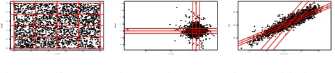
After transforming the distribution of the data into a joint uniform distribution, one can partition the uniformly distributed data into |C| number of cells as explained in Definition1; for example, from the Abalone dataset two RVs, Length and Shell Weight, are partitioned using uniform grid as shown in Figure 7.

0.0 0.2 0.4 0.6 0.8 1.0

0.0

0.2

0.4

0.6

0.8

1.0

Length

Shell.w

eight

Fig. 7. Uniform space

−10 −5 0

−4

−2

0

2

4

6

8

Length

Shell.w

eight

Fig. 8. Indep. space

0.1 0.2 0.3 0.4 0.5

0.05

0.10

0.15

Diameter

Height

Fig. 9. Original space

If we inverse transforms cells in the uniform domain space (Figure 7) back into the independent space (Figure 8) or into the original space (Figure 9), the size of the corresponding cells of the latter two domain spaces might shrink or expand. Recall that Disjoint Tree-based index approaches divide the data space into several cells that have different sizes but contain approximately an equal number of data points. Hence, while avoiding building and maintaining a tree-like data structure, we manage to partition the non-uniform domain space (Figure 8 and 9) in the same way as tree-based approaches.

B. Computing ExactkNN

During the above-mentioned transformation process, the domain spaces can be rotated, shrunk or stretched. Hence, as the Euclidean distance between any two points in the original space will be different than the Euclidean distance between the corresponding mapped points in the independent space (and similarly for the uniform space), only data points from the original domain space must be considered when the Euclidean distance metric is used to compute kNN queries. However, in-spite of the discrepancy of the distance in the three domain spaces, data points that lie in a given cell in original space their corresponding points in the independent (or uniform) space also lie within the corresponding cell in the independent (uniform) space. We base our transformation on this proposition by providing the Lemma1.

Lemma 1. For all data points that reside within a cell in the uniform space, their corresponding data points lie within the

boundaries of the corresponding cell in the independent and original spaces.

Proof: Letui be the value of theithdimension of a data point uthat lies in cell Cuni in the uniform space such that

[cuni min

i ≤ ui ≤ cuni maxi ] where cuni mini and cuni maxi are minimum and maximum values of the ith dimension of

Cuni_{, respectively. Let data pointybe the point resulting from} transforminguto the independent space withyibeing its value in ith _{dimension and cell C}ind _{resulting from transforming}

Cuni _{to the independent space with c}ind min

i and cind maxi are minimum and maximum values of the ith _{dimension of}

cind_{. Similarly, consider a cellC}org _{and data pointx created} by transformingCindandyto the original space, respectively. We shall first prove that a point belongs to Cind _{iff it belongs} toCuni. Then, by the transitivity, it is sufficient to show that a point belongs to Corg _{iff it belongs toC}ind_.

Case 1: Independent and Uniform Data Spaces.We need to prove that [cind min

i ≤yi≤cind maxi ]is true. Each RV of the uniform space is a cdf of a RV in the independent space:

cuni mini ≤ui≤cuni maxi ⇔

FY(Y ≤cind mini )≤FY(Y ≤yi)≤FY(Y ≤cind maxi ).

Since cdf is a monotonic increasing function and letφbe the inverse of cdf,we obtain that:

φ(cuni min_i )≤φ(ui)≤φ(cuni maxi )

⇔F_Y−1(Y ≤cind min_i )≤F_Y−1(Y ≤yi)≤FY−1(Y ≤c ind max

i )

⇔cind min_i ≤yi ≤cind maxi .

Case 2: Independent and Original Data spaces.We now prove that data point x lies within Corg _{iff y lies within}

Cind. Without loss of generality, consider that the data points

corg min_,xandcorg max_{are perpendicular andc}org min_and

corg maxare located on the boundaries ofCorg. Consider that

cind min _andcind max _{are corresponding points toc}org min

andcorg max_{, respectively, and are located on the boundaries}

of Cind_{. To proof by contradiction, let us assumex does not} lie within Corg _{when y lies within C}ind_{. Since A}−1 _{is the}

inverse of the whitening matrix in (2), we have that:

(corg min_i > xi)∨(xi> corg maxi )⇔

((A−1cind min)i0>(A−1y)i0)∨((A−1y)i0>(A−1cind max)i0)

By multiplying both sides byA, we obtain:

((AA−1cind min)i0>(AA−1y)i0)

∨((AA−1y)i0>(AA−1cind max)i0)

⇔((Icind min)i0>(Iy)i0)∨((Iy)i0>(I−1cind max)i0)

⇔(cind min_i > yi)∨(yi > cind maxi ).

The last equivalence does not hold when y lies within Cind_; hence our assumption that xdoes not lie withinCorg_wheny lies within Cind _{must be wrong. That is, x lies withinC}org iffy lies withinCind.

neighbouring cells is strait-forward. For instance, if cells are represented by their lower-left coordinate, the lower-left coordinates of the neighbouring cells can be computed by adding or subtracting the rwidth/height of the grid-cells (see Definition 1) to the ith_{dimension of the lower-left coordinate} of the given cell. At this point, it is worth mentioning that while memory hungry indexes are not required in the uniform space, but only data points from original space are needed for computing kNN queries. Therefore, to compute exact kNN without having memory hungry index, we transform the data to the uniform space and then partition the data space adopting a uniform-grid. But now, each cell of the uniform space stores the corresponding data points from the original space.

At first glance, such a design, i.e., a hybrid of the uniform and original domain spaces, might seem counter-intuitive be-cause usually, e.g. as in tree-based index approaches, only the original domain space is used. However, it should be noted that the lower-left coordinate of cells in the original space can be defined as a function of the lower-left coordinate of a corresponding cell in the uniform space as follows:

x=A−1K(u), (6)

where x is a lower-left coordinate of a cell in the original space, A−1 _{the inverse of the whitening matrix, K is a}

function (inverse cdf of RVs) that transforms back the RVs of the uniform space to the RVs of the independent space, and u is a lower-left coordinate of a corresponding cell in the uniform space. Thus, this can be seen as representing the

unequal-sized cells of the original space byequal-sized cells

of the uniform space.

IV. DATA ANDQUERYPROCESSING

We now describe the technical details of our proposed solu-tion. First, we discuss the creation of the STOS, then elaborate on how the STOS is used duringkNN query processing.

A. The STOS Methodology

The methodology in STOS can be split into two phases: data pre-processing and data organisation.

Data Pre-processing Phase. The steps in this phase are:

1) Using a MapReduce (MR) job, draw a random sample from the input dataset and count the total number of data points in the input dataset.

2) Operating on that sample, determine the correct number of GMM componentsM using the BIC, and then compute the mean vector µm, covariance matrix Σm, and the positive mixing weight πm of each clusterm.

3) For each cluster m, determine the whitening matrix A

(eq. (2)), de-correlate each cluster and transform the joint distribution of the de-correlated cluster into a joint mv uniform distribution.

4) Run pairwise dependence test at 95% level of accuracy for every transformed cluster; if the test fails either start from Step (2) using a different number of clusters M or reduce the level of accuracy.

5) Finally, use the positive mixing weights, average number of data points to be stored per cell (defined by a user), and the total number of data points in the input dataset

to determine the cell width for each transformed cluster (definition 1).

Data Organisation Phase. This phase consists of a MR job, where the mappers go through the points at their input and for each of these points, they:

1) Assign the data point to a cluster using a naive Bayesian algorithm.

2) Transform it to the uniform space using the statistical parameters of the cluster as computed in the Data Pre-processing Phase.

3) Assign it to a cell within the cluster, based on definition 1 and definition 2.

4) Finally, emit a key-value pair, where the key is a con-catenation of the cluster ID and the coordinates of the lower-left corner of the cell in the uniform space, and the value is the data point in the original space. The reducers also compute per-cluster metadata (MBRs) that contain the minimum and maximum value for every dimension of each cluster.

To expedite the query processing process, the reorganised data output by the above reducers must not stored in flat files, instead, in a table in the HBase. The schema used follows the aforementioned design; i.e., each row in this table has a rowkey that is the concatenation of a cluster ID and the lower-left coordinates of a cell in the uniform space, and contains a single column with all data points (in the original space) mapped to that cell. Moreover, instead of inserting the data points into the table one by one, the standard HBase bulk loading [5] technique is used.

B. Query Processing

When a query point q from a kNN query arrives at the system then the following steps are processed in the STOS:

1) We compute the distance betweenqand the MBR of each cluster (definition 3). Then, the closest cluster is selected. 2) The query point qis transformed into the uniform space, using the statistical parameters of the selected cluster, thus, resulting in a new pointquni_.

3) This new point is mapped to a cell in the cluster using definition 2 and, thus, the rowkey of the corresponding row in HBase is computed.

4) The contents of the above cell are retrieved from HBase and an initial kNN answer is computed, using the Eu-clidean distance betweenqand the retrieved data points.

Ifk > α(whereαis the (average) number of data points

per cell – definition 1), then we further retrieve as many neighbouring cells as necessary to ensure we fetch at least

k data points.

5) We then compute the distance,ρ, betweenqand thekth data element of the initialkNN answer, and draw a hyper-square whose centre is qand whose width is 2×ρ. 6) Finally, all rows that intersect and/or covered by the

hyper-square are retrieved and the final kNN result is computed and returned.

V. PERFORMANCEEVALUATION

A. Experimental setup

64GB RAM, and 2TB disk space.

1) Datasets: We use synthetic and real datasets of various sizes and dimensions in our experiments. The synthetic data has four clusters, of which three clusters have Gaussian distri-butions and one cluster has lognormal distribution, i.e., whose logarithm is Gaussian distribution. Based on the distribution of the synthetic data we generated three datasets. The first synthetic dataset contains around 8 billion points (total size of approx. 250GB), the second one includes 16 billion points (total size of approx. 500 GB), and the third one around 32 billion points (total size of approx. 1TB). Moreover, we use two real datasets from the UCL machine learning data repository: Istanbul stock exchange national 100 index [2] and Activity Recognition system based on Multisensor data fusion (AReM) [28]. To compare fairly with COWI, which is a QT-based approach, as it is already known that QT has poor applicability in high dimensions [32], we only consider the first two dimensions of the Istanbul dataset, and from the AReM dataset, we take the first and third dimensions of two the activ-ities (cycling and walking). In addition, we present the query performance of our method in high dimensions: six and nine dimensions from the AReM and Istanbul datasets, respectively. In order to generate (relatively) large-scale datasets and in light of the fact that available real-world datasets are typically of small sizes, we proceeded as follows: We generated six (2-d) datasets based on the parameters of the two real datasets (a practice that is prevalent in the related literature; e.g., see [21]). The first three datasets were generated based on the Istanbul dataset and contain 8, 16 and 32 billion data points, respectively. Three more datasets were generated based on the ARem dataset, containing also 8, 16 and 32 billion data points, respectively. The dataset sizes are approximately 250GB, 500GB, and 1TB for the 8, 16, and 32 billion data points, respectively. Given standard replication factors in the NoSQL and HDFS stores used by the STOS, these datasets reach the near-maximum available storage space. For higher dimensional data, we generated six datasets. Three datasets were generated based on AReM (6-d) and the dataset sizes are approximately 250GB, 500GB, and 1TB that contain 2.6, 5.33, and 10.6 billion data points, respectively. Three more datasets were generated based on the Istanbul (9-d) dataset that contained 1.7, 3.5 and 7.1 billion data points and the sizes are approximately 250GB, 500GB, and 1TB, respectively.

2) Queries and Performance metrics:

Queries.10k queries per dataset were generated and used for the performance evaluations that follow. For each query, a query point was generated uniformly at random and the system was asked for the kNN data points per dataset for this query point. This was repeated for each value ofk∈ {10,100,1000}.

Performance Metrics.We measure the STOS building time in minutes (min) and the coefficient of variation (COV) defined as the ratio: sd/E to measure the load-balancing of cells, where sd is the standard deviation of the number of points per cell and E is the average number of points per cell. Moreover, we measure memory requirements (in megabytes) to store STOS structure. To estimate the time to recover from failure, we measure STOS loading time in milliseconds (ms). Furthermore, after executing all queries sequentially, we compute the average query response time in ms per value of

k. To measure the network overhead during query processing,

(a) Creation/Building Time (b) HBase Bulk-Loading Time

Fig. 10. STOS vs. COWI Creation/Index Building/Storing – AReM datasets

we consider the average number of rows (cells) retrieved and the average number of data points accessed per query.

As mentioned earlier, it is generally accepted that build-ing indexes for competbuild-ing kNN processing methods is an expensive process and fraught with difficulties. For instance, we were not able to index the datasets using the publicly available codes of SHadoop and Simba. Hence, we compare our approach against COWI. Note that [7] already showed that COWI achieves approximately three orders of magnitude better performance compared to SHadoop and Simba. In the same work, COWI was shown to enjoy a better query performance than CONI (as CONI stores the index in HBase table, thus, requiring extra HBase accesses to read index data). It is hence sufficient to compare STOS against only COWI.

B. Performance Assessment: STOS vs Index Overheads

Figure 10(a) shows the STOS building times vis-a-vis the COWI index building times for different sizes of the AReM datasets. The COWI indexing time is roughly five times higher than that of STOS. In the literature, it is well-known that QT has high index building time, while Uniform Grid has a relatievely low index construction time [32]. Hence, the results of this experiment are as expected confirming that this still holds in STOS and COWI.

We also use the standard HBase bulk loading [5] technique to load the STOS-organised data into an HBase table. If the distribution of the row-keys of the HBase table is uniform, then the [5]-based loads are very efficient. Otherwise, a human ex-pert is required to manually split the regions of the HBase table to expedite the bulk-loading process. Likewise, as shown in Figure 10(b), STOS’s uniform distribution blends excellently with the existing techniques and has a better bulk-loading process than COWI: COW I M an depicts the case when COWI’s regions of the HBase table are partitioned manually, whereas COW I van stands for no manually partitioning of the regions. Note: it is not always straightforward to partition a non-uniformly distributed row-keys set into equal-sized par-titions manually.

Moreover, we measure the time recovery from failure (index or STOS loading time) for different dataset sizes as shown in Figure 11(a). In COWI, 6 sec to 26 sec are needed to load the index in memory. In addition, the index loading time increases linearly with the size of a dataset. The STOS loading time, on the other hand, is constant and dramatically lower, standing at 0.014 sec.

(a) Loading Time (b) Size In Memory(Bytes)

Fig. 11. STOS vs. COWI Loading – AReM datasets

(a) Creation/Index Building Time (b) HBase Bulk-Loading Time

Fig. 12. STOS vs. COWI Creation/Index Building/Storing – Istanbul datasets

11(b). In COWI, 0.60 GB to 2.4 GB are required to store the index of the datasets. On the other hand, the STOS’s space requirement is constant and dramatically (approximately three orders of magnitude) smaller, standing at 0.0012 GB for the different sizes of the dataset.

The index loading time and space requirements of COWI might seem to be small, in absolute numbers. However, it is worth mentioning that the space requirement of COWI is around 0.25% of the size of the dataset and we observe a linear increase of index loading time w.r.t. the dataset size. That is, if the dataset grows to petabytes then tens of GBs would be required. Furthermore, w.r.t. index loading times, given the linear increase observed for COWI, for a 1PB dataset, circa 7 hours would be needed to load the index.

The results for the Istanbul datasets are very similar, lead-ing to the same conclusions as the AReM datasets. Although a detailed discussion is omitted for space limitations, we show the STOS and COWI-index building times, HBase bulk loading times, index loading times and memory footprints in Figures 12(a), 12(b), 13(a), and 13(b), respectively.

C. Performance Assessment: Query Performance

We now turn to assessing query processing performance. As shown in Figure 14(a), we compare the kNN query response time of STOS against COWI based on the 250GB, 500GB and 1TB AReM-derived datasets. We measured the

kNN query response time in milliseconds (ms) for different values of k. In STOS, the query response time varies from 10ms to 29ms, while in COWI, the query response time is roughly similar and ranges from 8ms to 39ms. The results clearly indicate that STOS has better or similar performance compared to COWI, and both approaches show excellent scal-ability, i.e., very small query response times despite significant increases in the dataset size.

To further assess the query processing performance, we measure the average number of rows accessed per query, as

(a) Creation Time (b) Size In Memory(Bytes)

Fig. 13. STOS vs. COWI Loading – Istanbul datasets

(a) Query Response Times (b) Average # of Rows Accessed Per Query

Fig. 14. Query Processing Times and Accessed Data (Rows) – AReM datasets

shown in Figure 14(b), for different dataset sizes and values of k. STOS accesses on average 1.18 rows per query when

k=10 (with, on average, 2000 data points are stored per row) and for k=100 and k=1000 on average 1.64 and 3.35 rows were accessed, respectively. COWI accessed on average 1.15, 1.54, and 3.34 rows fork=10,k=100 andk=1000, respectively, when on average 2000 data points are stored per row. This demonstrates that COWI accessed roughly the same number of rows, but in both methods, the size of the dataset has no significant impact on the average number of rows accessed per query. The average number of rows per query is affected by the value ofk; i.e., large values ofk produce large query ranges.

On the other hand, as shown on Figure 15(a), on average, STOS accessed a smaller number of data points per query than COWI. Initially, this seems counter-intuitive because one can ask how can COWI access more data points while accessing a similar number of rows as STOS? Note that, even though both methods contain on average the same number of data points, as shown in Figure 15(b), the coefficient of variation (COV), which measures the variation around the mean number of points per row across rows, in STOS is 2% while in COWI is between 36% to 45%. This presents also independent evidence as to the ability of STOS to partition the space equitably, with cells having nearly-equal sizes. This is significant since, as we have found, partition sizes affect directly the load balancing among the processes tasked with building the tree indexes or STOS itself and the query processing times. Therefore, STOS building processes are more robust (less likely to hang during MR) and query processing times are more predictable as evidenced by the COV values. The query performance results for the Istanbul dataset are very similar; Figures 16(a), 16(b) and 17 show query response times, average number of rows accessed per query and the average number of data points accessed per query respectively.

(a) Average # of Data Points Ac-cessed per Query

(b) Coefficient of Variation of Num-ber of Data Points Per Cell

Fig. 15. Query Processing Costs – AReM datasets

(a) Query Response Times (b) Average # of Rows Accessed Per Query

Fig. 16. Query Processing Costs: Query Processing Times and Accessed Data (Rows) – Istanbul datasets

increasing dataset sizes, with STOS having a clear edge.

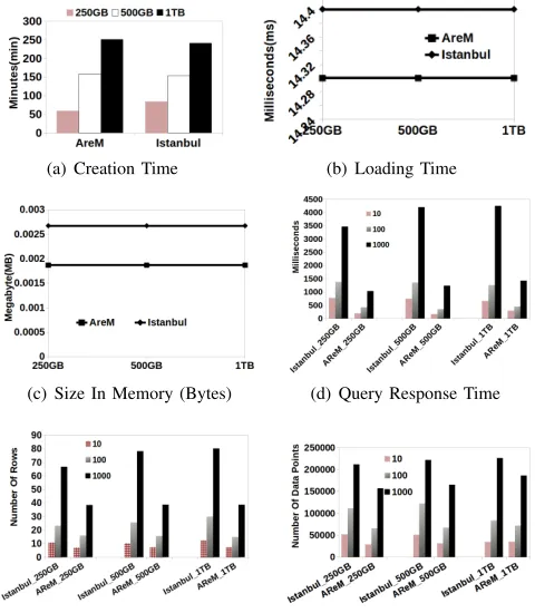
D. Performance Assessment: STOS in High Dimensions

In the related work section, we discussed the largely-held view that QT indexes are not appropriate for datasets with high data dimensionality. This is due to the fact that QT divides a cell into 2d _{sub-cells and creates too many nearly empty} cells in high d dimensional space. Hence, during the query processing most of the points in the QT will be accessed and, thus, the performance is similar to exhaustive search.

In our context, we assess the behaviour of STOS when data dimensionality increases. As shown in Figure 18(a), we focus on STOS building time and show how it is affected by the six dimensions of the AReM dataset and nine dimensions of the Istanbul dataset. Note that the creation time of STOS is not affected by the number of dimensions as the times required for 6-d, 9-d and 2-d datasets are quite similar. On the other hand, index loading time (Figure 18(b)) and memory footprint (Figure 18(c)) are not affected by the size of the datasets. We observe a slight increase in memory requirement, from 1.8 KB to 2.6 KB, as the data dimension increases from 6-d to 9-d. We also notice a slight increase in index loading time as the number of dimensions increases.

As shown in Figure 18(d), the query response time of dataset AReM ranges from 166ms to 1425ms; whereas for dataset Istanbul from 773ms to 4246ms. Again, the query response time does not show significant change with the different size of datasets, but the number of dimensions and different values ofksignificantly influence the query response time, as expected. Similarly, Figures 18(e) and 18(f) illustrate the average number of rows and data points accessed per query, respectively. Note, as the data dimensionality increases, the average number of rows and data points accessed per query increase significantly. However, STOS manages to process

Fig. 17. Average # of Data Points Accessed per Query – Istanbul Datasets

(a) Creation Time (b) Loading Time

(c) Size In Memory (Bytes) (d) Query Response Time

(e) Average # of Rows Accessed Per Query

(f) Average # of Data Points Accessed Per Query

Fig. 18. STOS vs High-dimensional Data – Istanbul (9-d) and AReM (6-d)

kNN queries on average from hundreds of milliseconds to a few seconds for the 6-d and 9-d datasets.

VI. CONCLUSIONS

of magnitude. Additionally, STOS memory footprint remains (nearly) constant as dataset sizes grow, unlike traditional tree-based indexes. Furthermore, the times required to build STOS are smaller by several orders of magnitude compared to traditional tree-index building times. At the same time, STOS is able to surgically access and transfer very small data chunks during query processing, thus, achieving very small query processing times. The above facts are critical in ensuring even higher overallkNN query processing efficiency and scalability. We have showcased the viability of STOS and substantiated the above claims using extensive experimentation over several real-world (big) datasets of various dimensions.

REFERENCES

[1] A. Aji, F. Wang, H. Vo, R. Lee, Q. Liu, X. Zhang, and J. Saltz. Hadoop GIS: A high performance spatial data warehousing system over MapReduce. PVLDB, 6(11):1009–1020, 2013.

[2] O. Akbilgic, H. Bozdogan, and M. E. Balaban. A novel hybrid rbf neural networks model as a forecaster. Statistics and Computing, 24(3):365– 375, 2014.

[3] A. M. Aly, A. S. Abdelhamid, A. R. Mahmood, W. G. Aref, M. S. Has-san, H. Elmeleegy, and M. Ouzzani. A demonstration of AQWA: Adap-tive query-workload-aware partitioning of big spatial data. PVLDB, 8(12):1968–1971, 2015.

[4] M. Armbrust et al. Spark sql: Relational data processing in spark. In Proc. ACM SIGMOD Intl. Conf. on Management of Data (SIGMOD), pages 1383–1394, 2015.

[5] X. Bao, L. Liu, N. Xiao, F. Liu, Q. Zhang, and T. Zhu. Hconfig: Resource adaptive fast bulk loading in hbase. InProc. IEEE Intl. Conf. on Collaborative Computing (CollaborateCom), pages 215–224, 2014. [6] J. L. Bentley. Multidimensional binary search trees used for associative

searching. Communications of the ACM, 18(9):509–517, 1975. [7] A. Cahsai, N. Ntarmos, C. Anagnostopoulos, and P. Triantafillou.

Scaling k-nearest neighbours queries (the right way). In Proc. IEEE Intl. Conf. on Distributed Computing Systems (ICDCS), pages 1419– 1430, 2017.

[8] S. Cambanis, S. Huang, and G. Simons. On the theory of elliptically contoured distributions. Journal of Multivariate Analysis, 11(3):368 – 385, 1981.

[9] A. Cary, Y. Yesha, M. Adjouadi, and N. Rishe. Leveraging cloud computing in geodatabase management. InGranular Computing (GrC), 2010 IEEE International Conference on, pages 73–78. IEEE, 2010. [10] G. Casella and R. Berger. Statistical inference, brooks/cole pub. Co,

Pacific Grove, CA, 1990.

[11] J. Chen. Optimal rate of convergence for finite mixture models. The Annals of Statistics, pages 221–233, 1995.

[12] W. J. Cody. Rational chebyshev approximations for the error function. Mathematics of Computation, 23(107):631–637, 1969.

[13] J. Dean and S. Ghemawat. MapReduce: a flexible data processing tool. Communications of the ACM, 53(1):72–77, 2010.

[14] A. P. Dempster, N. M. Laird, and D. B. Rubin. Maximum likelihood from incomplete data via the em algorithm. Journal of the Royal Statistical Society. Series B (Methodological), 39(1):1–38, 1977. [15] A. Eldawy, L. Alarabi, and M. F. Mokbel. Spatial partitioning

tech-niques in SpatialHadoop. PVLDB, 8(12):1602–1605, 2015.

[16] A. Eldawy and M. F. Mokbel. A demonstration of SpatialHadoop: An efficient MapReduce framework for spatial data. PVLDB, 6(12):1230– 1233, 2013.

[17] R. A. Finkel and J. L. Bentley. Quad trees a data structure for retrieval on composite keys. Acta informatica, 4(1):1–9, 1974.

[18] C. Genest and A.-C. Favre. Everything you always wanted to know about copula modeling but were afraid to ask. Journal of hydrologic engineering, 12(4):347–368, 2007.

[19] L. George. HBase: the definitive guide. O’Reilly Media, Inc., 2011. [20] A. Guttman. R-trees: A dynamic index structure for spatial searching.

InProc. ACM SIGMOD Intl. Conf. on Management of Data (SIGMOD), pages 47–57, 1984.

[21] D. Han and E. Stroulia. Hgrid: A data model for large geospatial data sets in hbase. InProc. IEEE Intl. Conf. on Cloud Computing (CLOUD), pages 910–917, 2013.

[22] Y.-T. Hsu, Y.-C. Pan, L.-Y. Wei, W.-C. Peng, and W.-C. Lee. Key formulation schemes for spatial index in cloud data managements. In Proc. IEEE Intl. Conf. on Mobile Data Management (MDM), pages 21–26, 2012.

[23] T. Huang, H. Peng, and K. Zhang. Model selection for gaussian mixture models.arXiv preprint arXiv:1301.3558, 2013.

[24] S. T. Leutenegger, M. A. Lopez, and J. Edgington. STR: A simple and efficient algorithm for R-tree packing. In Proc. IEEE Intl. Conf. on Data Engineering (ICDE), pages 497–506, 1997.

[25] M. Lichman. UCI machine learning repository, 2013.

[26] G. J. McLachlan and K. E. Basford. Mixture models: Inference and applications to clustering, volume 84. Marcel Dekker, 1988. [27] S. Nishimura, S. Das, D. Agrawal, and A. El Abbadi. MD-HBase:

Design and implementation of an elastic data infrastructure for cloud-scale location services. Distrib. Parallel Databases, 31(2):289–319, 2013.

[28] F. Palumbo, C. Gallicchio, R. Pucci, and A. Micheli. Human activity recognition using multisensor data fusion based on reservoir computing. Journal of Ambient Intelligence and Smart Environments, 8(2):87–107, 2016.

[29] S. T. Rachev, C. Menn, and F. J. Fabozzi. Fat-tailed and skewed asset return distributions: implications for risk management, portfolio selection, and option pricing, volume 139. John Wiley & Sons, 2005. [30] N. Roussopoulos, S. Kelley, and F. Vincent. Nearest neighbor queries.

ACM SIGMOD Record, 24(2):71–79, 1995.

[31] G. Schwarz et al. Estimating the dimension of a model. The annals of statistics, 6(2):461–464, 1978.

[32] H. Singh and S. Bawa. A survey of traditional and MapReduce-based spatial query processing approaches.ACM SIGMOD Record, 46(2):18– 29, 2017.

[33] M. Sklar. Fonctions de r´epartition `a n dimensions et leurs marges. Universit´e Paris 8, 1959.

[34] M. Tang, Y. Yu, Q. M. Malluhi, M. Ouzzani, and W. G. Aref. Locationspark: A distributed in-memory data management system for big spatial data. PVLDB, 9(13):1565–1568, 2016.

[35] J. Wang, W. Liu, S. Kumar, and S.-F. Chang. Learning to hash for indexing big dataa survey. Proceedings of the IEEE, 104(1):34–57, 2016.

[36] F. Xiao. A Spark based computing framework for spatial data. ISPRS Annals of Photogrammetry, Remote Sensing and Spatial Information Sciences, pages 125–130, 2017.

[37] D. Xie, F. Li, B. Yao, G. Li, L. Zhou, and M. Guo. Simba: Efficient in-memory spatial analytics. InProc. ACM Intl. Conf. on Management of Data (SIGMOD), pages 1071–1085, 2016.

[38] S. You, J. Zhang, and L. Gruenwald. Large-scale spatial join query processing in cloud. In Proc. IEEE Intl. Conf. on Data Engineering Workshops (ICDEW), pages 34–41, 2015.

[39] J. Yu, J. Wu, and M. Sarwat. Geospark: A cluster computing framework for processing large-scale spatial data. InProc. SIGSPATIAL Intl. Conf. on Advances in Geographic Information Systems, page 70, 2015. [40] M. Zaharia, M. Chowdhury, M. J. Franklin, S. Shenker, and I. Stoica.