On the UV compactness and morphologies of typical Lyman α emitters from z ∼ 2 to z ∼ 6

On the UV compactness and morphologies of typical

Lyman-

α

emitters from

z

∼

2

to

z

∼

6

Ana Paulino-Afonso

1

,

2

,

3

?

, David Sobral

3

,

4

, Bruno Ribeiro

5

, Jorryt Matthee

4

,

S´

ergio Santos

3

, Jo˜

ao Calhau

3

, Alex Forshaw

3

, Andrea Johnson

3

, Joanna Merrick

3

,

Sara P´

erez

1

,

2

,

3

, Oliver Sheldon

3

1_{Instituto de Astrof´ısica e Ciˆencias do Espa¸co, Universidade de Lisboa, OAL, Tapada da Ajuda, PT1349-018 Lisboa, Portugal} 2_{Departamento de F´ısica, Faculdade de Ciˆencias, Universidade de Lisboa, Edif´ıcio C8, Campo Grande, PT1749-016 Lisboa, Portugal} 3_{Department of Physics, Lancaster University, Lancaster, LA1 4YB, UK}

4_{Leiden Observatory, Leiden University, P.O. Box 9513, NL-2300 RA Leiden, The Netherlands} 5_{Centro de Computa¸c˜ao Gr´afica, CVIG, Campus de Azur´em, PT4800-058 Guimar˜aes, Portugal}

15 September 2017

ABSTRACT

Lyman-α (Lyα) is, intrinsically, the strongest nebular emission line in actively

star-forming galaxies (SFGs), but its resonant nature and uncertain escape fraction limits its applicability. The structure, size, and morphology may be key to understand the

escape of Lyα photons and the nature of Lyα emitters (LAEs). We investigate the

rest-frame UV morphologies of a large sample of ∼4000 LAEs from z ∼ 2 to z ∼ 6,

selected in a uniform way with 16 different narrow- and medium-bands over the full

COSMOS field (SC4K, Santos et al. in prep.). From the magnitudes that we measure

from UV stacks, we find that these galaxies are populating the faint end of the UV luminosity function. We find also that LAEs have roughly the same morphology from

z ∼ 2 to z ∼ 6. The median size (re ∼ 1 kpc), ellipticities (slightly elongated with

(b/a) ∼0.45), S´ersic index (disk-like withn.2), and light concentration (comparable

to that of disk or irregular galaxies, with C ∼2.7) show little to no evolution. LAEs

with the highest equivalent widths (EW) are the smallest/most compact (re∼0.8kpc,

compared to re∼1.5kpc for the lower EW LAEs). In a scenario where galaxies with

a high Lyα escape fraction are more frequent in compact objects, these results are a

natural consequence of the small sizes of LAEs. When compared to other SFGs, LAEs are found to be smaller at all redshifts. The difference between the two populations changing with redshift, from a factor of∼1at z&5to SFGs being a factor of∼2−4

larger than LAEs for z .2. This means that at the highest redshifts, where typical

sizes approach those of LAEs, the fraction of galaxies showing Lyαin emission should

be much higher, consistent with observations.

Key words: galaxies: evolution – galaxies: high-redshift – galaxies: star formation – galaxies: structure

1 INTRODUCTION

In the Λ-Cold Dark Matter framework, galaxies form through the coalescence of small clumps of material (see e.g.

Somerville & Dav´e 2015and references therein). This means that the first objects which can be called galaxies are to be young, small, and with low stellar mass content. The search

? _{E-mail: [email protected]}

for these building blocks of current day galaxies has been pursued intensively in the past decades (see e.g.Bromm & Yoshida 2011;Stark 2016).

Because of its intrinsic brightness, this search usually explores the presence of the Lyman-α (Lyα) emission line (e.g.Partridge & Peebles 1967;Schaerer 2003). This line can be observed in the optical and near-infrared when emitted from2 <z .8sources and it is proven to be a successful probe to identify and confirm high-redshift galaxies. From narrow-band surveys (e.g.Rhoads et al. 2000;Ouchi et al.

©0000 The Authors

2008,2010;Matthee et al. 2016,2017;Sobral et al. 2017b) to spectroscopic detection and confirmation of high-redshift candidates (e.g. Martin & Sawicki 2004; Ono et al. 2012;

Bacon et al. 2015;Le F`evre et al. 2015;Wisotzki et al. 2016), we have now access to large samples of young galaxies in the early Universe.

The physical properties of Lyα emitting galaxies (LAEs) have been intensively studied (e.g.Erb et al. 2006;

Gawiser et al. 2006,2007;Pentericci et al. 2007;Ouchi et al. 2008;Lai et al. 2008; Reddy et al. 2008; Finkelstein et al. 2009;Kornei et al. 2010;Guaita et al. 2011;Nilsson et al. 2011;Acquaviva et al. 2012;Oteo et al. 2015; Hathi et al. 2016; Matthee et al. 2016). Some works find them to be typically young, with low stellar masses, and scarce dust presence (e.g. Erb et al. 2006; Gawiser et al. 2006, 2007;

Pentericci et al. 2007; Oteo et al. 2015), while others indi-cate a more diverse population (e.g.Shapley et al. 2003;Lai et al. 2008;Reddy et al. 2008;Finkelstein et al. 2009;Kornei et al. 2010;Nilsson et al. 2011;Acquaviva et al. 2012;Hathi et al. 2016). The different properties of this population may be due to their particular selection method, as LAEs are similar to other line-emission selected galaxies atz∼2and different from colour-selected galaxies at the same redshifts (e.g.Oteo et al. 2015;Hagen et al. 2016). Evolution can also play a role in the different observed properties of LAEs with more evolved galaxies having Lyαemission driven by differ-ent mechanisms than those that dominate LAEs at higher redshifts. For e.g.,Santos et al.(in prep.) show a strong in-crease in the fraction of Active Galactic Nuclei (AGN) in luminous LAEs fromz∼4−5toz∼2−3.

A possible explanation to the diverse nature of LAEs is linked to the complicated nature of the radiative transfer process itself. To escape the region it originated from, Lyα photons are frequently scattered (with random walks up to several kpc) before they escape towards our line of sight (e.g.Zheng et al. 2011;Dijkstra & Kramer 2012;Lake et al. 2015; Gronke et al. 2015, 2016). This recurrent scattering increases the chance of the photon to be destroyed through dust absorption (e.g. Neufeld 1991; Laursen et al. 2013). This picture also means that the particular orientation of the emission path relative to the geometrical distribution of gas and dust in the emitting region is important to consider whether or not we are able to observe the line in emission. Some simulations of isolated disk galaxies have shown that the likelihood of observation of Lyα is correlated with the disk inclination relative to our line of sight (Verhamme et al. 2012;Behrens & Braun 2014). From an observational per-spective, the Lyα escape fraction (ratio of observed to in-trinsic flux in emission) is loosely correlated with the galax-ies’ star formation rate (SFR) and dust attenuation (e.g.

Hayes et al. 2010, 2011; Atek et al. 2014; Matthee et al. 2016;Trainor et al. 2016;Oyarz´un et al. 2017). The column density of HI seems to be another physical quantity that determines the rate of escape of Lyαphotons (e.g. Shibuya et al. 2014a,b;Henry et al. 2015), and it also correlates with equivalent width (EW,Sobral et al. 2017b;Verhamme et al. 2017).

The complex process of Lyα escape naturally means that obtaining a complete census of the galaxy population at a given epoch is challenging. To understand the mecha-nisms that allow Lyαphotons to escape it may be important to correlate the morphology of star-forming regions traced

by UV continuum emission of young stars with the observed from Lyαphotons. This will allow one to constrain the ge-ometry requirements for Lyα to escape from galaxies and further our knowledge of population bias when using selec-tions solely based on this emission line. To gain insight on the mechanisms of Lyα escape it is thus crucial that we characterize the morphology of these sources.

Several samples of LAEs have been studied in terms of their rest-frame UV morphologies atz>2(e.g.Pirzkal et al. 2007; Taniguchi et al. 2009; Bond et al. 2009, 2011, 2012;

Gronwall et al. 2011; Kobayashi et al. 2016). In the local Universe, where rest-frame UV observations are scarce, there is one study based on the Lyα Reference Sample (LARS,

¨

Ostlin et al. 2014 though the sample is Hαselected), that characterizes the morphology of these sources (Guaita et al. 2015). Observations show that LAEs are typically small, of-ten compact objects (half-light radius around 1 kpc), which undergo no evolution in the first 1 to 3 billion years of the Universe (z ∼ 2−6, e.g Venemans et al. 2005; Mal-hotra et al. 2012). This scenario is in stark contrast with the stronger evolution in galaxy sizes observed in other pop-ulations observed at similar epochs such as Lyman-break galaxies (LBGs) and other star-forming galaxies (e.g. Fer-guson et al. 2004;Bouwens et al. 2004; van der Wel et al. 2014;Shibuya et al. 2016;Paulino-Afonso et al. 2017). This can potentially be explained due to the low stellar mass na-ture of LAEs when compared to other galaxies. However, most studies on SFGs explore the size evolution in stellar mass bins and find stronger size evolution nonetheless (e.g.

van der Wel et al. 2014).

One interesting property of LAEs is that the Lyα emis-sion region is often found to be more extended (in a dif-fuse halo) than the stellar UV continuum emission (e.g.

Rauch et al. 2008;Matsuda et al. 2012;Momose et al. 2014;

Matthee et al. 2016; Wisotzki et al. 2016; Sobral et al. 2017b). The process responsible for such observations is thought to be the scattering of photons by neutral HI gas around galaxies at high redshift (e.g.Zheng et al. 2011), but could also be due to cooling, satellites, and fluorescence (e.g.

Mas-Ribas et al. 2017). Additionally, there are evidences for a correlation between Lyα line luminosity and galaxy UV continuum size (e.g.Hagen et al. 2014).

It is still unclear whether LAEs are a special subset of galaxies, if they rather just trace an early phase of galaxy formation, or if they are a consequence of different orienta-tion angles from which Lyαphotons peer through. To make progress, we have to look at their morphological proper-ties across cosmic time. In addition to that, it is necessary to compare to other galaxy populations (e.g. LBGs, HAEs, SFGs) for an understanding on how these populations are linked.

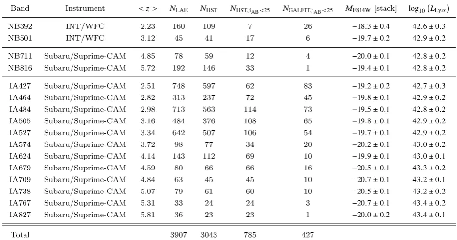
contex-Table 1.The full sample of Lyαemitters selected with the 16 narrow- and medium-bands used in this work. The<z>column shows the average redshift for the LAEs that fall in the filter. TheNLAEcolumn shows the total number of LAEs detected in the NB/IB images. The NHST column shows those who are covered by the HST/ACS F814W imaging survey. The NHST,iAB<25column shows the number of LAEs with available HST data with brighter thaniAB<25. The NGALFIT,iAB<25 column shows the number of bright LAEs for which

GALFIThas converged. TheMF814W[stack] column shows the absolute magnitude in thei-band of the median stacks (see Section3.4) which should closely trace MUV. The log10 LLyα shows the median Lyαluminosity of each sample (values derived byMatthee et al. 2016;Santos et al. 2016,in prep.;Sobral et al. 2017b).

Band Instrument <z> NLAE NHST NHST,iAB<25 NGALFIT,iAB<25 MF814W[stack] log10 LLyα

NB392 INT/WFC 2.23 160 109 7 26 −18.3±0.4 42.6±0.3

NB501 INT/WFC 3.12 45 41 17 6 −19.7±0.2 42.9±0.2

NB711 Subaru/Suprime-CAM 4.85 78 59 12 4 −20.0±0.1 42.8±0.2

NB816 Subaru/Suprime-CAM 5.72 192 146 33 1 −19.4±0.1 42.8±0.2

IA427 Subaru/Suprime-CAM 2.51 748 597 62 83 −19.2±0.2 42.7±0.3

IA464 Subaru/Suprime-CAM 2.82 313 237 72 45 −19.8±0.1 42.9±0.2

IA484 Subaru/Suprime-CAM 2.98 713 563 114 73 −19.5±0.1 42.8±0.2

IA505 Subaru/Suprime-CAM 3.16 484 376 108 65 −19.8±0.1 42.9±0.2

IA527 Subaru/Suprime-CAM 3.34 642 507 106 54 −19.7±0.1 42.9±0.2

IA574 Subaru/Suprime-CAM 3.72 98 77 34 20 −20.2±0.1 43.0±0.2

IA624 Subaru/Suprime-CAM 4.14 143 112 69 10 −19.9±0.1 43.0±0.1

IA679 Subaru/Suprime-CAM 4.59 80 66 66 16 −20.5±0.1 43.3±0.2

IA709 Subaru/Suprime-CAM 4.84 63 45 45 10 −20.7±0.1 43.2±0.1

IA738 Subaru/Suprime-CAM 5.07 79 61 60 10 −20.5±0.1 43.2±0.2

IA767 Subaru/Suprime-CAM 5.31 33 24 24 3 −20.7±0.1 43.4±0.2

IA827 Subaru/Suprime-CAM 5.81 36 23 23 1 −20.0±0.2 43.4±0.1

Total 3907 3043 785 427

tualize our results within recent results from the literature on morphology of high redshift galaxies.

The paper is organized as follows. In Section2we de-scribe the data used for the detection and characterization of LAEs that are the object of study in this work. We present our methodology to study the structural parameters of high redshift galaxies in Section 3. The results obtained for the LAEs samples are reported in Section4. We discuss the im-plications of our results in the context of early galaxy as-sembly in Section5. Finally, in Section6we summarize our conclusions.

Magnitudes are given in the AB system (Oke & Gunn 1983). All the results assume aΛ-CDM cosmological model withH0=70.0km s−1Mpc−1,Ωm=0.3, andΩΛ=0.7.

2 THE SAMPLE OF LYαEMITTERS AT Z∼2−6

The use of narrow-band images to target the Lyαline at spe-cific redshift windows has been widely used in recent years (e.g. Rhoads et al. 2000;Ouchi et al. 2008; Matsuda et al. 2011;Konno et al. 2014,2016;Trainor et al. 2016;Santos et al. 2016;Matthee et al. 2016;Sobral et al. 2017b). In this paper we use a dataset obtained with the Wide Field Cam-era at the Isaac Newton Telescope (WFC/INT) and with the Suprime-Cam at Subaru Telescope that cover the full COSMOS field (seeScoville et al. 2007).

We analyse a sample of ∼4000 Lyα-selected galaxies spanning a wide redshift range of z ∼2−6(SC4K, Santos et al. 2016,in prep.;Sobral et al. 2017b). The sources were

detected using a compilation of 16 narrow- and medium-band images taken with the Subaru and the Isaac Newton telescopes. Briefly, sources were classified as Lyα emitters if they satisfied all the following conditions: 1) significant detection in a narrow/medium band with equivalent width cuts being of 25/50˚A, respectively; 2) presence of a Lyman break blue-ward of the respective narrow/medium band; 3) no strong red colour in the near-infrared, typical of a red star or lower redshift interlopers. For the full selection criteria we refer the reader toSantos et al.(in prep.). The galaxies in our sample probe aroundL_Ly∗ _αat all redshifts (Santos et al. in prep.).

2.1 INT/WFC

We use data from the recent CAlibrating LYMan-α with Hα survey (CALYMHA,Matthee et al. 2016;Sobral et al. 2017b). This survey aims at detecting LAEs at z = 2.23

(but also allow the study of other emission lines, see e.g.

Stroe et al. 2017a,b) combined with new observations at

reso-lution (0.3300/pixel) and their Point Spread Function (PSF -which ranges from1.8−2.000). Fluxes are computed in300 cir-cular apertures. Candidate Lyαemitters are selected to have rest-frame equivalent widths (EW0) greater than 25˚A ( So-bral et al. 2017b;Matthee et al. 2017). We perform an addi-tional colour selection aimed at excluding potential interlop-ers at the redshifts we are probing (seeSobral et al. 2017b;

Matthee et al. 2017with respect to NB392 and NB501 colour selections, respectively). In the end, our WFC/INT sample has a total 160 LAEs atz=2.23and 45 LAEs atz=3.1in the COSMOS region (see Table1).

2.2 Subaru/Suprime-Cam

We explore deep data obtained Subaru Suprime-Cam (Miyazaki et al. 2002) in the COSMOS field. We have re-duced and analysed archival data of 2 narrow-band and 12 medium-band filters that are listed in Table 1. The reduc-tion procedure is that described by Matthee et al.(2015) and Santos et al.(2016). The extraction of LAEs from the reduced data follows closely the method described in Sec-tion 2.1 using the appropriate broad band filter data cor-responding to each filter for continuum estimation (optical and near-infrared images/catalogues described byTaniguchi et al. 2007,2015andCapak et al. 2007). We note that the selection criteria for narrow-band detected LAEs impose a rest-frame equivalent widths EW0 > 25˚A (Santos et al. 2016). For medium-band filters, the rest-frame equivalent width cut is at EW0 >50˚A. The number of detected LAEs

for each processed narrow- and medium-band is shown in Table1.

3 METHODOLOGY

To quantify the morphological properties of any given source it is common to fit a parametric model to the observed light profile. In the particular case of galaxy modelling, theS´ er-sic (1968) profile is the most common model assumed (e.g.

Davies et al. 1988;Caon et al. 1993;Andredakis et al. 1995;

Moriondo et al. 1998;Simard 1998;Khosroshahi et al. 2000;

Graham 2001;M¨ollenhoff & Heidt 2001;Trujillo et al. 2001;

Peng et al. 2002; Blanton et al. 2003;Trujillo et al. 2007;

Wuyts et al. 2011; van der Wel et al. 2014;Shibuya et al. 2016) and which is also used to model LAEs (e.g. Pirzkal et al. 2007; Bond et al. 2009; Gronwall et al. 2011). The S´ersic model can be described as

I(r)=Ieexp[−κ(r/re)1/n+κ], (1) where the S´ersic index n describes the shape of the light profile,reis the effective radius of the profile,Ieis the surface brightness at radiusr=re, andκis a parameter coupled to nsuch that half of the total flux is enclosed withinre. This profile assumes two characteristic models for specific values ofn: exponential disk, ifn=1, and ade Vaucouleurs(1948) profile, ifn=4, best suited for elliptical galaxies and galactic bulges.

An alternative method, relying solely on the observed properties of each object, is to use a non-parametric ap-proach to the morphological characterization (see e.g. Abra-ham et al. 1996;Bershady et al. 2000;Conselice et al. 2000;

Conselice 2003; Lotz et al. 2004). These methods offer re-liable estimates even in the case of extremely irregular ob-jects, but fail to account for instrumental effects (such as PSF broadening) and are more susceptible to biases induced by low S/N conditions.

To study the rest-frame UV morphological properties of galaxies at high redshift, the availability of high resolution observations is required. Thus, we limit all our analysis to where HST/ACS F814W images available (COSMOS sur-vey, Scoville et al. 2007; Koekemoer et al. 2007). We use

1000×1000cut-outs of the HST/ACS F814W (Scoville et al. 2007; Koekemoer et al. 2007) centred on each LAE. The cut-outs are produced from the COSMOS HST/ACS im-ages available on the COSMOS archive. These imim-ages have a typical PSF FWHM of∼0.0900, a pixel scale of0.0300/pixel, and a limiting point-source depth AB(F814W) = 27.2 (5σ). These images are probing the near to far UV for the sources in our sample (on average∼2000˚A rest-frame).

3.1 Structural parameter estimation

The retrieval of structural parameters based on S´ersic pro-files is done using the publicly available GALFIT (Peng et al. 2002,2010), a stand-alone program aimed at two di-mensional decomposition of light profiles through model fit-ting. In addition to the parameters described in Equation

11, 2D models need 4 additional quantities: the model cen-tral position,xcandyc, the axis ratio of the isophotes,b/a, and respective position angle, θP A, i.e. the angle between the major axis of the ellipse and the vertical axis.

To run_GALFITeffectively, it is necessary that we pro-vide an initial set of parameters. To speed up convergence and minimize the occurrence of unrealistic solutions, it is important that these first guesses provide a good approxi-mation of the light profile. To do so, we use the source extrac-tion softwareSExtractor(Bertin & Arnouts 1996), which can be tuned to produce the parameter set that will be used as input to GALFIT. To fit our galaxies, we use cut-outs centred on each target. The size of the cut-outs was cho-sen so that we achieve good speed performance and to allow

GALFITto simultaneously fit the residual sky emission. To account for the instrumental PSF effects on the ob-served light profile, we provide PSF images associated with each individual galaxy. We use the HST/ACS PSF profiles that were created withTinyTim (Krist 1995) models and described byRhodes et al.(2006,2007). The PSF model ac-counts for pixel-to-pixel variation inside the CCD and the different telescope focus value for each COSMOS tile obser-vation. We used the segmentation map produced by

SEx-tractorat the time of the estimation of the initial parame-ters to create a mask image that flagged all pixels belonging to neighbouring galaxies, preventing them to influence the model of the object of interest. We mask all sources at a dis-tance greater than 1.500 from the target RA, DEC (∼10-13 kpc). We use a morphological dilation (kernel of3×3pixels) to smooth the individual masked regions and include in the same mask lower flux pixels in the outskirts that are below the_SExtractordetection threshold.

1 _In

−1 0 1 −1.5

−1.0 −0.5 0.0 0.5 1.0 1.5

Δ

δ

[

00

]

IA464 53900

5 kpc

Compact

−1 0 1

Δα [

00

_]

IA464 15390

5 kpc

Disky

−1 0 1

IA527 117114

5 kpc

Irregular

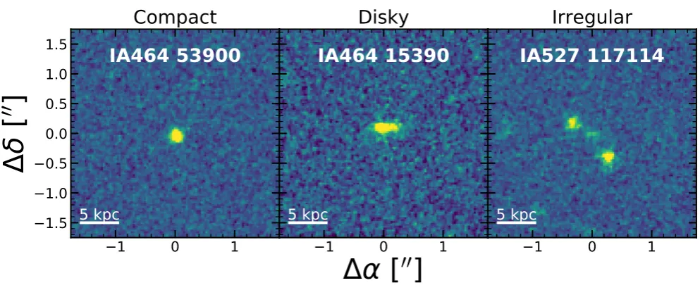
Figure 1. Examples of LAEs for each of the morphological classes that we have defined for this study. The classes are displayed from left to right in terms of decreasing compactness: 1) bright round sources with compact profiles; 2) disk-like sources; and 3) irregular/mergers/clumpy sources.

Irregular, complex, and/or sources detected at low S/N are excluded from the final sample as_GALFITfailed to con-verge on meaningful structural parameters. Note, however, that we also visually classify all sources; see Section3.3.

3.2 Light concentration

As not all our sources are well fit with a symmetric model (∼ 45%), we opted to estimate the light concentration of each source by using a non-parametric approach. We have computed their concentration of light parameter, C ( Con-selice et al. 2000; Conselice 2003). We used SExtractor

20% and 80% light radius (defined with the parameter

PHOT FLUXFRAC) and directly computed the value as

C=5 log₁₀

r80

r₂₀

, (2)

where r80 and r20 are the 80% and 20% light radius,

re-spectively. This parameter measures the rate of decay of the light profile of galaxies in concentric elliptical apertures and allows us to understand if galaxies have lower or higher sur-face density of stellar emission in the near- and far-UV. Such measure can be linked to the type of star-formation occur-ring in LAEs which would, in turn, shed some light on the mechanisms linked to the formation of new stars that may boost the escape of Lyαphotons.

3.3 Visual classification

We complemented the quantification of LAE morphology with the visual classification of the rest-frame UV shapes for all sources with iAB < 25 and HST coverage. We

visu-ally classify galaxies in a simple numerical scheme from 0 to 4 in terms of decreasing compactness: 0) corresponding to faint point-like sources; 1) slightly more extended/bright round/not extended sources; 2) disk-like sources; and 3) ir-regular/mergers/clumpy sources (see Figure1). Each object

was classified independently by three different team mem-bers and we combined the final classification by averag-ing over all classifications. For simplicity, we group classes 0 and 1 as compact sources, 2 as disky, and 3 as irregu-lar/clumpy/mergers.

3.4 Stacks of Lyα emitters

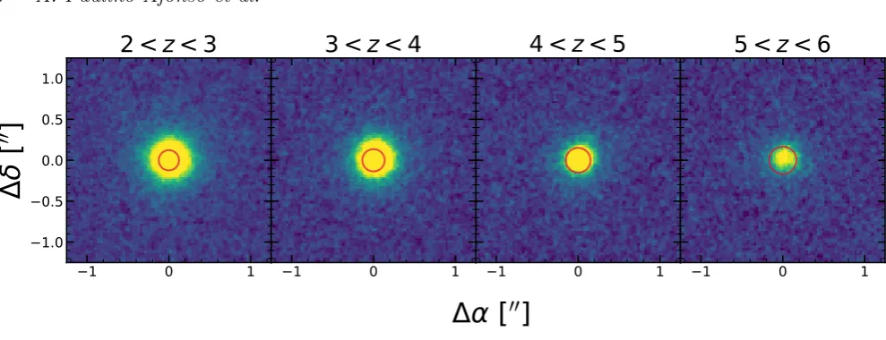
The major goal of stacking is to get measurements of the typical galaxy, while not being biased by the ones that are brightest in F814W. We have stacked all detected LAEs with available HST/ACS F814W images using the median flux per pixel, centred at Lyαdetection. We have also performed an image shift (typically . 0.500on the detected sources) since the image coordinates are measured on ground based images and we observe some deviations when seeing them at HST resolution. The resulting stacks, in specific ranges of redshift, Lyα equivalent width, and Lyα luminosity, are shown in Figure2(see alsoA2).

We show in Table1 the absolute magnitude of these stacks as observed in HST/ACS F814W. These have typical values of ∼26 and correspond to absolute magnitudes, in F814W, ranging fromM_i,NB392=−18.3(at low redshift) up toMi,IA827=−20.0(at high redshift). These magnitudes are

typically 1 to 2 magnitudes lower thanM_UV∗ at all redshifts (e.g.Reddy & Steidel 2009;Bouwens et al. 2015;Finkelstein et al. 2015;Parsa et al. 2016;Alavi et al. 2016).

One of the quantities that is affected by the uncertain-ties on the astrometry of LAEs and a possible mismatch between the peak of Lyα emission and the UV emission (see e.g.Shibuya et al. 2014a) is the size of the produced light profiles. As we combine astrometric errors from a large number of sources, the profile tends to enlarge. To correct for this, we have used the subset for which we have UV de-tections in HST (iAB<25) to compute the difference when

−1 0 1 −1.0

−0.5 0.0 0.5 1.0

Δ

δ

[

00

]

2 < z < 3

−1 0 1

3 < z < 4

−1 0 1

4 < z < 5

−1 0 1

5 < z < 6

Δα [

00

_]

Figure 2.Examples of LAE stacks for each of the bins that we use in this study in terms of redshift. In each panel, the intensity levels range from -3σskyto 15σsky, whereσskyis the sky rms. The red circle in each panel has a physical radius of 1 kpc.

we produce stacks with an effective radius ∼1.1-1.5 times larger. We have computed individual corrections for each of the stacks and morphological quantitiesre, n, C, and applied to all values reported in this work (see e.g. FigureA1).

4 MORPHOLOGICAL PROPERTIES OF LAES

We have full morphological information on 427 galaxies across2.z.6due to GALFIT convergence issues on low S/N galaxies and bright near-point like objects. For visual classification and light concentration parameters, we have results for the 785 galaxies with HST images. In the next subsections we will detail the rest-frame UV morphological properties of each sample and compare it to the strength of the Lyαemission. We stress that all our results presented in the next subsection are limited to LAEs withiAB ≤25. For

a summary of our findings, see Table2. We have excluded X-ray detected AGNs from the sample (seeCalhau et al. in prep.for details on AGN selection).

4.1 S´ersic indices and sizes

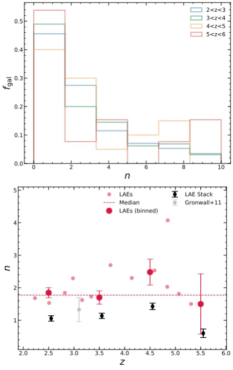
In Figure 3 we show the distribution of S´ersic indices and corresponding median of the population. It is readily notice-able that most LAEs have disk-like profiles (n <1.5) with fractions ranging from∼39%at4<z <5up to∼54%at

5<z<6(at2<z<3and3<z<4the fractions are of 45% and 49%, respectively). We note that there are LAEs with high values of the S´ersic index. Such cases can be related to galaxies with evident interactions, asymmetric morpholo-gies, or compact spheroidal object which we can check with our visual morphological classification. We parametrize the redshift evolution as

X=β(1+z)α (3)

withα, βbeing the parameters to be fit andXthe dependent variable,nin this case. We find thatn∝ (1+z)−0.78±0.71for the median of the LAE population, which is consistent (at the∼1σlevel) with a scenario of no evolution in the light profiles of LAEs. We find that for the lower redshift bins,

our reported median values for the S´ersic index are in good agreement with those reported byGronwall et al.(2011). We find systematically lower S´ersic indices for measurements of stacks of LAEs than for individual detections. These dif-ference are related to the smoothing of the central region of the light profile caused by uncertainties on the astrome-try (in random directions) and Lyα-UV offset which dilute the light and make the profile shallower. Nonetheless, the reported trend is also consistent with little evolution with redshift.

We show in Figure4the overall properties of the LAE population in 4 bins spanning the redshift range2≤z≤6. One of the first results is that LAEs have similar size distri-butions at all redshifts, with most galaxies having effective radii smaller than 1.5 kpc, and with ∼ 20% as extended sources withrefrom 2-5 kpc. This similarity extends to the evolution on the median population sizes fromz∼6toz∼2, where we observe that LAEs are consistent with little to no evolution scenario in terms of their extent. These results are in agreement with previous results in the literature based on narrow-band selected LAEs (see e.g.Pirzkal et al. 2007;

Taniguchi et al. 2009;Bond et al. 2009,2011;Gronwall et al. 2011;Malhotra et al. 2012;Kobayashi et al. 2016). For the evolution of effective radius we find thatre∝ (1+z)−0.21±0.22. This roughly translates to a growth by a factor of∼1.2±0.2

for LAEs fromz∼6to z∼2(consistent with no evolution within1σ), which compares to a factor of∼2.3±0.15for a more general star forming population (see e.g.van der Wel et al. 2014;Ribeiro et al. 2016).

We find systematically higher values of the effective ra-dius or measurements of stacks of LAEs than for individual detections. We believe that this is in part due to the cen-tring errors mentioned above, but for which we have tried to correct. When deriving size evolution from the stacked pro-files we find thatre ∝ (1+z)−0.01±0.25, perfectly consistent with the lack of evolution we find for the median population evolution.

0 2 4 6 8 10

n

0.0 0.1 0.2 0.3 0.4 0.5

fgal

2<z<3 3<z<4 4<z<5 5<z<6

2.0 2.5 3.0 3.5 4.0 4.5 5.0 5.5 6.0

z

1 2 3 4 5

n

LAEs Median LAEs (binned)

LAE Stack Gronwall+11

Figure 3. S´ersic index median values of LAEs at 2 . z . 6. On the top panel we show the S´ersic index distribution of LAEs for each redshift bin considered. On the bottom panel we plot the evolution of the median S´ersic index of the distribution (our results in semi-transparent red circles for individual bands and large opaque red circles after binning in redshift) and compare our values to those reported byGronwall et al.(2011, grey pentagon). The red dashed line marks the median S´ersic index for individual LAEs at any redshift. The black diamonds show the S´ersic index of the stacked LAEs.

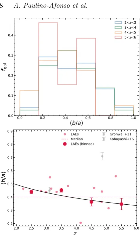
4.2 Ellipticities

The ellipticity of a source is defined as e =1− (b/a). We show in Figure 5 the results for the derived axis-ratio for the sources in our sample. We find that LAEs have no clear preference for an ellipticity value, with most of our sources lying at intermediate values 0.2<(b/a) <0.8. This implies that the detected LAEs do not have to be of a particular shape, which is expected given the randomness of the line-of-sight alignments that determine the 2D shape of each galaxy when viewed through an image. On a more interesting note, this also tells us that a specific alignment of the source with our line-of-sight is not required for it to be detected as a Lyαemitter. These results are in good agreement with mea-surements at 3 < z < 5 by Gronwall et al. (2011). Given

0 1 2 3 4 5

re[kpc]

0.0 0.1 0.2 0.3 0.4

fgal

2<z<3 3<z<4 4<z<5 5<z<6

2.0 2.5 3.0 3.5 4.0 4.5 5.0 5.5 6.0

z

0.5 1.0 1.5 2.0 2.5

re

[k

p

c]

LAEs Median LAEs (binned) LAE Stack

Pirzkal+07

Taniguchi+09 Bond+09,11 Gronwall+11 Malhotra+12 Kobayashi+16

Figure 4.Size properties of LAEs at 2 . z . 6. On the top panel we show the size distribution of LAEs for each redshift bin considered. On the bottom panel we plot the evolution of the median size of the distribution (our results in semi-transparent red circles for individual bands and large opaque red circles af-ter binning in redshift) and compare our values to those reported in the literature (in grey): square (Pirzkal et al. 2007); hexagon (Taniguchi et al. 2009); triangles (Bond et al. 2009,2011); pen-tagon (Gronwall et al. 2011); circles (Malhotra et al. 2012); and diamond (Kobayashi et al. 2016). The black solid line shows the best fit ofre ∝ (1+z)α. The red dashed line marks the median effective radius for individual LAEs at any redshift. The black diamonds show the effective radius of the stacked LAEs.

the constant S´ersic indices and the small sizes, our results thus hint that the high Lyαescape fractions of our sources are more of a consequence of their sizes and not orientation effects.

0.0 0.2 0.4 0.6 0.8 1.0

(b/a)

0.0 0.1 0.2 0.3 0.4

fgal

2<z<3 3<z<4 4<z<5 5<z<6

2.0 2.5 3.0 3.5 4.0 4.5 5.0 5.5 6.0

z

0.2 0.3 0.4 0.5 0.6 0.7 0.8 0.9

(b

/a

)

LAEs Median LAEs (binned)

Gronwall+11 Kobayashi+16

Figure 5.Axis-ratio median values of LAEs at 2.z .6. We plot the evolution of the median axis-ratio of the distribution (our results in semi-transparent red circles for individual bands and large opaque red circles after binning in redshift) and we compare our values to those reported in the literature (in grey): pentagon (Gronwall et al. 2011); and diamond (Kobayashi et al. 2016). The black solid line shows the best fit of(b/a) ∝ (1+z)α. The red dashed line marks the median axis-ratio for all LAEs at any redshift.

they useSExtractorto measure ellipticities that does not account for any PSF broadening which in the case of small galaxies, such as is typical of LAEs, it is natural that the shape is dominated by the PSF in its core, artificially lower-ing the ellipticity. Uslower-ing the parametrization of Equation3

we find thatb/a∝ (1+z)−0.46±0.16, which is marginally con-sistent with a constant ellipticity scenario (within3σ). This little or no evolution reinforces the idea that the galaxy ori-entation is not a main factor in driving the escape fraction for LAEs.

4.3 Concentration

In Figure 6 we investigate any evolution in terms of the light concentration of galaxies. It is rather stable atC∼2.7

with the exception of the value at4<z<5. The fact that

2.0 2.5 3.0 3.5 4.0 4.5 5.0 5.5 6.0

z

1.8 2.0 2.2 2.4 2.6 2.8 3.0

C

LAEs Median LAEs (binned)

LAE Stack Gronwall+11

Figure 6.Concentration median values of LAEs at2 .z .6. We plot the evolution of the median concentration of the distri-bution (our results in semi-transparent red circles for individual bands and large opaque red circles after binning in redshift) and compare our values to those reported byGronwall et al. (2011, grey pentagon). The red dashed line marks the median concen-tration for individual LAEs at any redshift. The black diamonds show the concentration of the stacked LAEs. The higher value of concentration for the stacked profiles is likely linked to the com-bination of the compact nature of these objects and the stacking method we use (see Section4.3for more details).

this parameter is strikingly similar, in its median evolution, with the S´ersic index is a possible indication that the galax-ies we are probing are rather symmetrical in nature. Both parameters provide a measure of the surface brightness con-centration and, in the case of a symmetrical S´ersic profile, it can be shown that C has a monotonic relation with n

(e.g.Graham & Driver 2005). We find that our results are also in good agreement with the findings byGronwall et al.

(2011). Using the parametrization of Equation3we find that

C∝ (1+z)0.04±0.09, fully consistent with a constant light con-centration across the entire redshift range. We observe a rise in light concentration for sources atz∼4−5, which is possi-bly related to an increase on the number of irregular galaxies that we observe. We note that the value at4<z<5is also potentially related to a shallower depth of the images for detection of Lyα(NB711 and IA709), which are more likely to pick sources with higher surface densities and thus higher values ofC are to be expected.

The values we find for the concentration of the stacked profiles are consistent with those we find for the median of the population. At the highest redshift, we find much lower concentrations which is potentially related to the higher number of undetected sources that populate this bin allied to the fact that this is also the bin with the fewer galaxies in the stack.

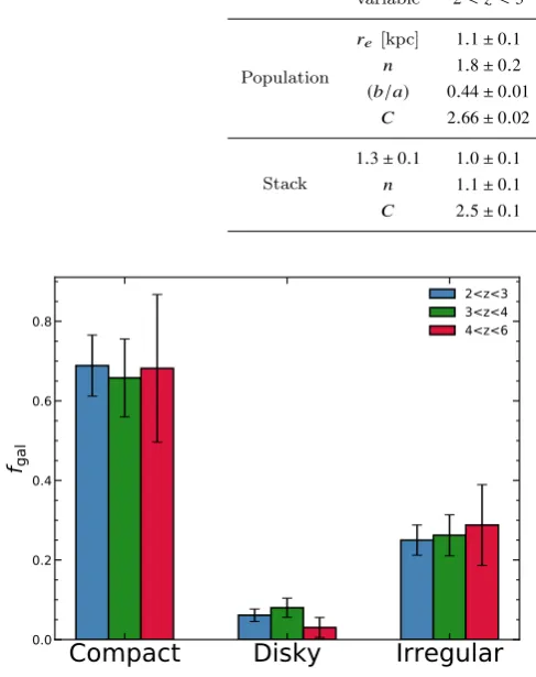
4.4 Morphological classes

Of the 1092 galaxies withiAB<25only 631 had good quality

Table 2.Median population and stack values as a function of redshift for the morphological quantities presented in this work.

variable 2<z<3 3<z<4 4<z<5 5<z<6

Population

re [kpc] 1.1±0.1 1.1±0.2 0.9±0.3 1.0±0.2 n 1.8±0.2 1.7±0.2 2.5±0.4 1.5±0.9

(b/a) 0.44±0.01 0.45±0.02 0.36±0.03 0.35±0.04 C 2.66±0.02 2.66±0.02 2.86±0.05 2.69±0.09

Stack

1.3±0.1 1.0±0.1 1.2±0.1 1.3±0.1

n 1.1±0.1 1.1±0.1 1.4±0.1 0.6±0.1 C 2.5±0.1 2.6±0.1 2.8±0.1 1.8±0.1

Compact

Disky

Irregular

0.0 0.2 0.4 0.6 0.8

fgal

2<z<3 3<z<4 4<z<6

Figure 7.Fraction of galaxies in each of the morphology classes from visual classification of LAEs at2.z.6.

visual classification. We find that the majority of our bright LAEs (∼67%) are found to be compact (point-like+elliptical class). Of the other classes, we find that irregular LAEs are ∼ 26%of our sample while disky galaxies amount to only ∼ 7% of the observed LAEs. These fractions are roughly constant, but we observe only a slight rise in the fraction of irregulars towards higher redshifts which can be expected of young galaxies in the earlier Universe (e.g. Buitrago et al. 2013;Jiang et al. 2013;Huertas-Company et al. 2015;Bowler et al. 2017).

4.5 The lack of evolution in LAE morphologies

We have shown in the previous sections the general prop-erties of LAEs in the sample we are studying and find that the morphology of this population of galaxies is rather sta-ble in this∼3 Gyr period. Since we find that there is not any strong evident evolution in all presented parameters, we opt to study the dependence of Lyαemission properties on the rest-frame UV morphology using the entire sample without discriminating between redshifts (with the majority of our sources being at z ∼2−3). This hypothesis will boost the number of sources to inspect such relations and thus uncover more effectively any underlying correlations that may exist. We are aware that our sample selection is not done in any absolute quantities (such as in Lyαluminosity orMUV)

and thus we may introduce some biases in our interpreta-tion of the redshift evoluinterpreta-tion of the presented quantities. We have tested our hypothesis of selection by comparing our re-sults using selections onlog₁₀(LLyα) >43 and MI <−20.5,

(MI is the absolute magnitude of the observed I band)

in-dependently. We can report that the lack of evolution in the reported morphological quantities is observed in these smaller subsets from our main sample, thus we opt to keep the apparent magnitude cut as our main selection.

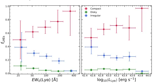
4.6 Morphology dependence on Lyα luminosity and equivalent width

After summarizing our findings on the morphological prop-erties across cosmic time for the LAEs in our sample, we now turn to the influence of morphology on the observed properties of the Lyα emission itself (line equivalent width and luminosity).

We show in Figure8the fraction of each morphological class as a function of line equivalent width and line lumi-nosity. We find that we have no disky galaxies at the lowest equivalent widths and that the irregular galaxies are less common at higher equivalent widths. These trends are ac-companied by a slight rise in the fraction of compact galaxies with line equivalent width. We also find that the brightest emitters are tendentiously more likely to be compact than their lower luminosity counterparts. We observe a decline in the fraction of irregular galaxies with line luminosity and a rather stable fraction of disky galaxies at all luminosities that we are probing.

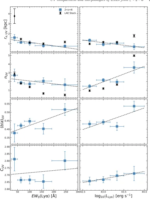
Our results on the relations between morphological quantities and Lyα emission properties are summarized in Figure9and in Table3.

25 50 100 200 400

EW

0.0 0.2 0.4 0.6 0.8 1.0

f

E

s

42.4 42.6 42.8 43.0 43.2 43.4 43.6 43.8 44.0

log10

₍

L

)

[erg s

]

Compact Disky Irregular

Figure 8.Fraction of LAEs of a given morphological class (compact as red circles, disky as green diamonds, and irregulars as blue squares) at2.z.6as a function of line equivalent width (left) and line luminosity (right).

since studies have shown that Lyαequivalent width traces the Lyαescape fraction (e.g.Sobral et al. 2017b;Verhamme et al. 2017). We highlight that the trend is also observed for the stacked profiles.

We plot in Figure9(second panel, left column) the re-lation between S´ersic index and Lyα equivalent width and find that there is a slight sign of a correlation between these two quantities. Our data suggests that at higher equivalent widths (EW0(Lyα)>200˚A) we are more likely to have

shal-lower profiles. This trend is also seen from the stacked pro-files albeit at systematically lower values of n(see Section

4.1).

A stronger correlation that we find is between the axis-ratio of the emission and the measured line equivalent width. In Figure9 (third panel, left column) we find that the strongest emitters (the ones with the largest equivalent width) tend to have rounder shapes (higher axis-ratios, lower ellipticities). These findings are in agreement with those re-ported byKobayashi et al.(2016) at z∼4.86. If we assume that the axis-ratio is a good proxy for galaxy inclination, we can explain the observed trend as a simple effect of ge-ometry due to the inclination of the disk with respect to our line of sight (see e.g.Verhamme et al. 2012;Behrens & Braun 2014). However, one must be cautious when compar-ing observations directly with simulations since the latter assume that the galaxy is a perfect flat disk and the former assumes that galaxies are symmetrical enough to be well fit by a parametric model, and either assumption has its draw-backs.

We finally explore the correlation between light con-centration and Lyαin Figure9(fourth panel, left column). Much like the case we presented for the S´ersic index, we

can-not infer conclusively about any correlation between these two quantities. We may tentatively say that galaxies with higher equivalent widths (EW0(Lyα) > 200˚A) are to be

more concentrated in term of the rest-frame UV emission when compared to their lower equivalent width counter-parts. The higher concentration value we have for the lower equivalent width bin is explained due to the lower number statistics of that bin. As stated in Section2, galaxies with

25<EW0(Lyα)<50˚A are only from narrow band data.

We attempt at a similar exercise as above and explore the possible correlations between the galaxy morphology and its observed Lyαline luminosity.

Concerning galaxy sizes there is an apparent downward trend for galaxies with 1042.5 . LLyα . 1044erg s−1 with

galaxies being smaller at higher luminosities (see Figure9, first panel, right column). This trend is not clear since there are some bin-to-bin variations that are mainly due to our small number of objects as well as the loose correlation that exists between these two quantities (for any luminosity bin there is a large spread in galaxy sizes). Interestingly we find an opposite trend when considering the sizes of the stacked profiles. We find this can be explained by an underlyingiAB

- Lyα line luminosity where the brightest galaxies on our sample in rest-frame UV are also the ones with the highest Lyαline luminosity. When stacking a large number of bright galaxies we are more likely to pick up extended lower surface brightness regions and thus get larger sizes.

EW

(Lyα) [Å]

1 2 3 4

r

V

[k

p

c]

2<z<6 LAE Stack

log

(

L

)

[erg s

]

EW

(Lyα) [Å]

1 2 3 4 5

n

V

log

(

L

)

[erg s

]

EW

(Lyα) [Å]

0.35 0.40 0.45 0.50 0.55

(b

/a

)

log

(

L

)

[erg s

]

50 100 150 200 250 300

EW

(Lyα) [Å]

2.60 2.65 2.70 2.75 2.80 2.85 2.90

C

V

42.5 43.0 43.5 44.0

log

(

L

)

[erg s

]

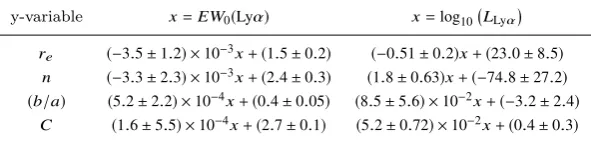
Table 3.Linear fits shown in Figure9. Each line represents a morphological quantity and in the second and third columns we show the parameters from the best fit for Lyαequivalent width and luminosity, respectively.

y-variable x=EW0(Lyα) x=log10 LLyα

re (−3.5±1.2) ×10−3x+(1.5±0.2) (−0.51±0.2)x+(23.0±8.5) n (−3.3±2.3) ×10−3x+(2.4±0.3) (1.8±0.63)x+(−74.8±27.2) (b/a) (5.2±2.2) ×10−4x+(0.4±0.05) (8.5±5.6) ×10−2x+(−3.2±2.4)

C (1.6±5.5) ×10−4x+(2.7±0.1) (5.2±0.72) ×10−2x+(0.4±0.3)

two quantities. Nevertheless, it is remarkable that the bright-est LAEs have such high S´ersic index (n∼3.5), correspond-ing to more classical elliptical profiles. This is a consequence of bright, small, and compact objects that are more likely to possess such profiles. We find the same response when looking at the values of the stacked LAEs, with high lumi-nosity LAEs (LLyα∼1043.75erg s−1) having higher values of

n∼4. We find the same trend when considering the stacked profiles, albeit at a shallower slope and systematically lower values ofn(see Section4.1).

When estimating the median axis ratio as a function of Lyαline luminosity (see Figure9, third panel, right column) we find the same trend as compared to the relation with line equivalent width. In this case, galaxies at higher luminosi-ties show less elongated shapes than their lower luminosity counterparts.

Finally, we show in Figure 9 (fourth panel, right col-umn) that there is a small but steady increase of the light concentration for our luminosity bins. This trend is less bro-ken that what is reported for the equivalent width of the Lyα line, but still points to a scenario where the brightest Lyα emitters are more likely to have high light concentration in their profiles (as also seen in the S´ersic index).

5 DISCUSSION

5.1 The lack of evolution in LAE morphology between z∼2−6

Our results regarding galaxy morphology as a function of redshift (see Section 4) indicate that LAEs have the same typical shape across the period we probe (z ∼2−6). This is reflected by the little to no variation in size, S´ersic index, axis-ratio, and light concentration parameters which is seen both in the median of the population as well as in the stacked profiles.

5.2 LAE sizes at z∼2−6

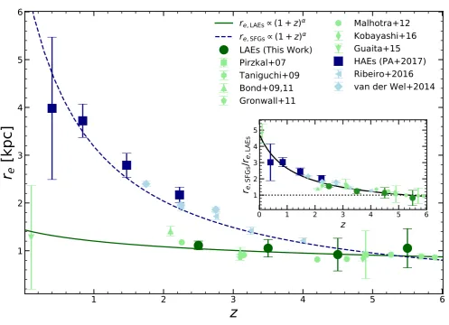
Finally, in Figure10we show our results for the evolution in rest-frame UV sizes of LAEs across cosmic time and compare our findings to previous studies (e.g.Taniguchi et al. 2009;

Bond et al. 2011,2012;Gronwall et al. 2011;Guaita et al. 2015; Kobayashi et al. 2016). Our median effective radius are in agreement with other size estimates of LAEs in the literature. Atz&4we find typical sizes ofre∼0.9kpc and atz∼2.2we find slightly larger galaxies with average sizes of

re=1.1kpc. We have attempted to fit a relation to our data points and find thatre ∝ (1+z)−0.21±0.22 (see Section4.1). This scenario, however, predicts slightly larger sizes atz∼0

than what have been reported for the LARS sample in the local Universe (Guaita et al. 2015), but within their reported dispersion. This scenario points to a lack of evolution on the sizes of LAEs sincez∼6. However, this reasoning hinges on the single point that we have atz∼0and which is derived from a heterogeneous sample of 14 galaxies only. To fully understand if LAEs evolve in size as hinted by the data atz∼2.5one would need larger samples betweenz=0−2, which are currently out of the scope of any instrument apart from HST/COS.

5.3 Relations between LAEs, HAEs, and UV-selected galaxies

When compared to the typical sizes of star-forming galaxies (selected as Hαemitters, HAEs) that have been studied in a previous work (Paulino-Afonso et al. 2017), we immediately see that the two populations are not alike in terms of their extent. Despite having only one common period with obser-vations of both populations (atz =2.23), where HAEs are almost two times larger than LAEs, our prediction of LAEs sizes at lower redshifts are consistently lower that what we report for the HAE population. This is even more contrast-ing if we include the sample atz∼0, where almost no evolu-tion is expected for the LAEs populaevolu-tion. This is potentially corroborated by the existence of green pea galaxies ( Carda-mone et al. 2009; Izotov et al. 2011) which are compact in nature and found to have Lyα detections and high Lyα escape fractions (e.g.Henry et al. 2015;Yang et al. 2016;

Verhamme et al. 2017).

We also use two recent and comprehensive studies on the evolution of UV-selected star-forming galaxies (van der Wel et al. 2014;Ribeiro et al. 2016, see alsoShibuya et al. 2015) that overlap both HAEs and LAEs that we have stud-ied to complement our observations. These confirm our find-ings that at z ∼ 2 the typical star-forming population is larger in size than the LAEs population (by a factor of∼3). However, we see that this difference fades away and, byz∼5, the two populations are indistinguishable from one another, in what their median extent is concerned. These results are in agreement with previous findings where both populations are compared (e.g.Malhotra et al. 2012).

con-1 2 3 4 5 6

z

1 2 3 4 5 6

r

e

[k

p

c]

re, LAEs∝ (1 + z)α

re, SFGs∝ (1 + z)α LAEs (This Work) Pirzkal+07 Taniguchi+09 Bond+09,11 Gronwall+11

Malhotra+12 Kobayashi+16 Guaita+15 HAEs (PA+2017) Ribeiro+2016 van der Wel+2014

0 1 2 3 4 5 6

z

1 2 3 4 5

r

FG

s

/r

,L

A

E

s

Figure 10.Size properties of LAEs at2.z.6. We plot the evolution of the median size of the distribution (our results in large green circles) and compare our values to those reported in the literature (in light green): square (Pirzkal et al. 2007); hexagon (Taniguchi et al. 2009); triangles (Bond et al. 2009,2011); circles (Malhotra et al. 2012); diamond (Kobayashi et al. 2016); and inverted triangle (Guaita et al. 2015). We show as blue squares the median size for a sample of HAEs selected at lower redshift using the same narrow band technique (Paulino-Afonso et al. 2017). We complement this figure with results for UV-selected star-forming galaxies from the literature (in light blue): large diamond (van der Wel et al. 2014) and left-facing triangle (Ribeiro et al. 2016). Finally, we show the derived size evolution of LAEs (green solid line) and SFGs (blue dashed line). The inset plot shows the estimated size ratio between SFGs and LAEs. Estimates point to SFGs being∼5times larger atz ∼0and of the same size as LAEs atz∼5.5. We hypothesize that Lyαselected galaxies are small/compact throughout cosmic time likely linked with the physical processes that drive Lyαescape. At higher and higher redshifts, typical SFGs start to have the typical sizes of Lyαemitters, which can be seen as an alternative explanation for the rise of the Lyαemitting fraction of SFGs/LBGs intoz∼6.

tent, metallicity, and star formation evolution) and we tend to observe less and less Lyαin emission, and observe large galaxies which are still actively forming stars but do not con-tribute to the global budget of the observed Lyαemission of the Universe. This decoupling of the two populations with respect to their median size occurs roughly ∼1 Gyr after the first galaxies are born. By arguing that the distinction between the two populations happens at the time where a galaxy has evolved for long enough not to be observed as a LAE any more, we can hypothesise that the life cycle of the Lyαemission of a galaxy is typically of the same scale. This means that we may expect on average every galaxy to be observed in Lyαemission for the first∼1 Gyr of its life.

We are aware that our scenario is grossly simplistic, but it finds support by other studies where LAEs are found to be

of low mass and low dust content (e.g.Gawiser et al. 2007;

Pentericci et al. 2007;Lai et al. 2008, see alsoErb et al. 2006;

Kornei et al. 2010;Hathi et al. 2016). However, there are a number of other studies that report conflicting evidence (e.g.

Finkelstein et al. 2009; Nilsson et al. 2011, see alsoReddy et al. 2008). The large diversity of results indicate a more intricate nature of LAEs, pointing to a scenario with possibly recurrent phases of Lyαemission throughout a galaxy’s life cycle.

renders them more likely to be observed as a LAE, as a consequence of Lyαescaping more easily in smaller galaxies. In the early Universe, typical SFGs have sizes comparable to Lyαemitters, which offers an alternative explanation for the rising fraction of the Lyα emitting SFGs/LBGs up to

z∼6(e.g.Hayes et al. 2011;Stark et al. 2011;Mallery et al. 2012;Cassata et al. 2015).

5.4 Visual morphology of LAEs

We show in Figure8that bright LAEs and high line equiva-lent width LAEs are more likely to be found with a compact shape. By relating the visual morphology with the struc-tural parameters that we have computed (see Section3) we can find some corroborating signs. Galaxies at the bright end of our LAE sample are found to be smaller, with higher S´ersic indices, rounder (higher axis-ratio) and with higher light concentrations. These characteristics are relatable to a classical small and round elliptical galaxy, which would be classified as compact given our classification scheme. Apart from the discrepancy on the S´ersic index, we see the same aforementioned trends in the relation of structural parame-ters with line equivalent width.

5.5 The geometric nature of Ly-α emission

We found some evidence to support that there are some ge-ometric requirements for the successful escape of Lyα pho-tons. In summary, compact and rounded objects are more likely to harbour conditions for such occurrence. This does not invalidate that there are other processes which con-tribute significantly to such event. The hinted correlations that we find are far from being a definite conclusion on this matter and certainly the existence of outflows, asymmetric, or lack of gas and dust distributions can contribute as well to the observation of Lyαin emission.

This assertion is supported by the relations we find be-tween light concentration and galaxy axial ratio with Lyα line equivalent width. As found bySobral et al.(2017a) the escape fraction of Lyαphotons correlates with the Lyα rest-frame equivalent width. So our results are pointing to the fact that galaxies that are rounder and with higher concen-trations of their light profile have potentially higher escape fractions. These results are in line with predictions from sim-ulations (e.g Verhamme et al. 2012), if we assume the the axis-ratio is a good proxy for galaxy inclination with respect to our line of sight. However, a scenario of compact objects with higher volume density of stars can reproduce similar results without the need to invoke galaxy inclination to ex-plain the observations. We believe the latter scenario is more likely the explanation for our results, since we do not expect the majority of our galaxies to have had the time to converge in a rotation supported disk for which the inclination would play a more prevalent role in the perceived escape fraction from our line of sight.

6 CONCLUSIONS

We present the morphological characterization of a large sample of ∼4000 LAEs and quantify their evolution in the first ∼3 Gyr of the Universe (2 . z . 6). We study the

correlation between the rest-frame UV morphology and the strength of the Lyαemission as a probe to the understand-ing of the mechanisms underlyunderstand-ing the escape of Lyαphotons from its host galaxy. Our results can be summarized as:

• UV sizes of LAEs are constant fromz∼2toz∼6with sizes ofre∼1.0±0.1kpc. We observe a rise in sizes towards lower redshifts (z ∼2), but the trend is shallow. The little to no evolution seems to hold even down toz∼0.

• At redshiftsz.5, LAEs have sizes that are consistently smaller than those reported for normal SFGs. The difference between the two populations gets more pronounced as we move towards lower redshifts, going from a factor of∼1 at

z &5to SFGs being a factor of ∼2−4larger than LAEs for z . 2. We hypothesize that the small/compact nature of LAEs is potentially linked to physical escape mechanisms of Lyα photons. In the early Universe, typical SFGs have sizes comparable to Lyα emitters, which offers an alterna-tive explanation for the rising fraction of the Lyα emitting SFGs/LBGs up toz∼6.

• The profiles of LAEs as seen from the rest-frame UV are remarkably constant fromz∼2up to z∼6withn∼1.7 be-ing slightly steeper than a pure exponential disk. The same scenario is seen in the evolution of the light concentration and axis ratio of LAEs.

• We find that most LAEs in our sample are compact in their morphology. The fraction of compact LAEs is larger at high line equivalent widths and also at high Lyαluminosity. • Lyα equivalent width seems to correlate stronger with the axis ratio and size of galaxies than any other morpho-logical parameter we have tested. Strong LAEs are found more likely in small and rounder galaxies (re∼0.8kpc and b/a∼0.5).

• The results that we report as the median properties of the population are corroborated by the morphological prop-erties of the stacked profiles of LAEs. This means that even when the image depth is increased, we find no difference with respect to the detected LAEs and discard the existence of an extended lower surface brightness region around UV-bright LAEs.

In broad terms, our results provide a global picture on the rest-frame UV morphology of LAEs in the early Uni-verse. We find that this particular population of galaxies does not evolve significantly in the first 3 Gyr of the Uni-verse and that it departs from the evolution of normal star-forming galaxies forz<4, in what galaxy sizes is concerned.

ACKNOWLEDGEMENTS

Isaac Newton Group in the Spanish Observatorio del Roque de los Muchachos of the Instituto de Astrofisica de Canarias. We are grateful to the CFHTLS, COSMOS-UltraVISTA, UKIDSS, SXDF and COSMOS survey teams. Without these legacy surveys, this research would have been impossible. This work was only possible by the use of the following

pythonpackages: NumPy & SciPy (Walt et al. 2011;Jones

et al. 2001), Matplotlib (Hunter 2007), and Astropy ( As-tropy Collaboration et al. 2013).

REFERENCES

Abraham R. G., van den Bergh S., Glazebrook K., Ellis R. S., Santiago B. X., Surma P., Griffiths R. E., 1996,ApJS,107, 1 Acquaviva V., Vargas C., Gawiser E., Guaita L., 2012,ApJ,751,

L26

Alavi A., et al., 2016,ApJ,832, 56

Andredakis Y. C., Peletier R. F., Balcells M., 1995,MNRAS,275, 874

Astropy Collaboration et al., 2013,A&A,558, A33

Atek H., Kunth D., Schaerer D., Mas-Hesse J. M., Hayes M., ¨

Ostlin G., Kneib J.-P., 2014,A&A,561, A89 Bacon R., et al., 2015,A&A,575, A75

Behrens C., Braun H., 2014,A&A,572, A74

Bershady M. A., Jangren A., Conselice C. J., 2000,AJ,119, 2645 Bertin E., Arnouts S., 1996, A&AS,117, 393

Blanton M. R., et al., 2003,ApJ,594, 186

Bond N. A., Gawiser E., Gronwall C., Ciardullo R., Altmann M., Schawinski K., 2009,ApJ,705, 639

Bond N. A., Gawiser E., Koekemoer A. M., 2011,ApJ,729, 48 Bond N. A., Gawiser E., Guaita L., Padilla N., Gronwall C.,

Cia-rdullo R., Lai K., 2012,ApJ,753, 95

Bouwens R. J., Illingworth G. D., Blakeslee J. P., Broadhurst T. J., Franx M., 2004,ApJ,611, L1

Bouwens R. J., et al., 2015,ApJ,803, 34

Bowler R. A. A., Dunlop J. S., McLure R. J., McLeod D. J., 2017, MNRAS,466, 3612

Bromm V., Yoshida N., 2011,ARA&A,49, 373

Buitrago F., Trujillo I., Conselice C. J., H¨außler B., 2013, MN-RAS,428, 1460

Calhau J., Sobral D., J. M., Santos S., Stroe A., Paulino-Afonso A., in prep., MNRAS

Caon N., Capaccioli M., D’Onofrio M., 1993,MNRAS,265, 1013 Capak P., et al., 2007,ApJS,172, 99

Cardamone C., et al., 2009,MNRAS,399, 1191 Cassata P., et al., 2015,A&A,573, A24 Conselice C. J., 2003,ApJS,147, 1

Conselice C. J., Bershady M. A., Jangren A., 2000,ApJ,529, 886 Davies J. I., Phillipps S., Cawson M. G. M., Disney M. J.,

Kib-blewhite E. J., 1988,MNRAS,232, 239 Dijkstra M., Kramer R., 2012,MNRAS,424, 1672

Erb D. K., Shapley A. E., Pettini M., Steidel C. C., Reddy N. A., Adelberger K. L., 2006,ApJ,644, 813

Ferguson H. C., et al., 2004,ApJL,600, L107

Finkelstein S. L., Rhoads J. E., Malhotra S., Grogin N., 2009, ApJ,691, 465

Finkelstein S. L., et al., 2015,ApJ,810, 71 Gawiser E., et al., 2006,ApJ,642, L13 Gawiser E., et al., 2007,ApJ,671, 278 Graham A. W., 2001,AJ,121, 820

Graham A. W., Driver S. P., 2005,Publ. Astron. Soc. Australia, 22, 118

Gronke M., Bull P., Dijkstra M., 2015,ApJ,812, 123

Gronke M., Dijkstra M., McCourt M., Oh S. P., 2016,ApJ,833, L26

Gronwall C., Bond N. A., Ciardullo R., Gawiser E., Altmann M., Blanc G. A., Feldmeier J. J., 2011,ApJ,743, 9

Guaita L., et al., 2011,ApJ,733, 114 Guaita L., et al., 2015,A&A,576, A51 Hagen A., et al., 2014,ApJ,786, 59 Hagen A., et al., 2016,ApJ,817, 79 Hathi N. P., et al., 2016,A&A,588, A26 Hayes M., et al., 2010,Nature,464, 562

Hayes M., Schaerer D., ¨Ostlin G., Mas-Hesse J. M., Atek H., Kunth D., 2011,ApJ,730, 8

Henry A., Scarlata C., Martin C. L., Erb D., 2015,ApJ,809, 19 Huertas-Company M., et al., 2015,ApJ,809, 95

Hunter J. D., 2007, Computing In Science & Engineering, 9, 90 Izotov Y. I., Guseva N. G., Thuan T. X., 2011,ApJ,728, 161 Jiang L., et al., 2013,ApJ,773, 153

Jones E., Oliphant T., Peterson P., et al., 2001, SciPy: Open source scientific tools for Python,http://www.scipy.org/

Khosroshahi H. G., Wadadekar Y., Kembhavi A., 2000,ApJ,533, 162

Kobayashi M. A. R., et al., 2016,ApJ,819, 25 Koekemoer A. M., et al., 2007,ApJS,172, 196 Konno A., et al., 2014,ApJ,797, 16

Konno A., Ouchi M., Nakajima K., Duval F., Kusakabe H., Ono Y., Shimasaku K., 2016,ApJ,823, 20

Kornei K. A., Shapley A. E., Erb D. K., Steidel C. C., Reddy N. A., Pettini M., Bogosavljevi´c M., 2010,ApJ,711, 693 Krist J., 1995, in Shaw R. A., Payne H. E., Hayes J. J. E., eds,

Astronomical Society of the Pacific Conference Series Vol. 77, Astronomical Data Analysis Software and Systems IV. p. 349 Lai K., et al., 2008,ApJ,674, 70

Lake E., Zheng Z., Cen R., Sadoun R., Momose R., Ouchi M., 2015,ApJ,806, 46

Laursen P., Duval F., ¨Ostlin G., 2013,ApJ,766, 124

Law D. R., Steidel C. C., Shapley A. E., Nagy S. R., Reddy N. A., Erb D. K., 2012,ApJ,759, 29

Le F`evre O., et al., 2015,A&A,576, A79

Lotz J. M., Primack J., Madau P., 2004,AJ,128, 163

Malhotra S., Rhoads J. E., Finkelstein S. L., Hathi N., Nilsson K., McLinden E., Pirzkal N., 2012,ApJ,750, L36

Mallery R. P., et al., 2012,ApJ,760, 128 Martin C. L., Sawicki M., 2004,ApJ,603, 414

Mas-Ribas L., Dijkstra M., Hennawi J. F., Trenti M., Momose R., Ouchi M., 2017,ApJ,841, 19

Matsuda Y., et al., 2011,MNRAS,410, L13 Matsuda Y., et al., 2012,MNRAS,425, 878

Matthee J., Sobral D., Santos S., R¨ottgering H., Darvish B., Mobasher B., 2015,MNRAS,451, 400

Matthee J., Sobral D., Oteo I., Best P., Smail I., R¨ottgering H., Paulino-Afonso A., 2016,MNRAS,458, 449

Matthee J., Sobral D., Best P., Smail I., Bian F., Darvish B., R¨ottgering H., Fan X., 2017, preprint, (arXiv:1702.04721) Miyazaki S., et al., 2002,PASJ,54, 833

M¨ollenhoff C., Heidt J., 2001,A&A,368, 16 Momose R., et al., 2014,MNRAS,442, 110

Moriondo G., Giovanardi C., Hunt L. K., 1998,A&AS,130, 81 Neufeld D. A., 1991,ApJ,370, L85

Nilsson K. K., ¨Ostlin G., Møller P., M¨oller-Nilsson O., Tapken C., Freudling W., Fynbo J. P. U., 2011,A&A,529, A9

Oke J. B., Gunn J. E., 1983,ApJ,266, 713 Ono Y., et al., 2012,ApJ,744, 83

¨

Ostlin G., et al., 2014,ApJ,797, 11

Oteo I., Sobral D., Ivison R. J., Smail I., Best P. N., Cepa J., P´erez-Garc´ıa A. M., 2015,MNRAS,452, 2018

Ouchi M., et al., 2008,ApJS,176, 301 Ouchi M., et al., 2010,ApJ,723, 869

Parsa S., Dunlop J. S., McLure R. J., Mortlock A., 2016,MNRAS, 456, 3194

Partridge R. B., Peebles P. J. E., 1967,ApJ,147, 868

Paulino-Afonso A., Sobral D., Buitrago F., Afonso J., 2017, MN-RAS,465, 2717

Peng C. Y., Ho L. C., Impey C. D., Rix H.-W., 2002, AJ,124, 266

Peng C. Y., Ho L. C., Impey C. D., Rix H.-W., 2010, AJ,139, 2097

Pentericci L., Grazian A., Fontana A., Salimbeni S., Santini P., de Santis C., Gallozzi S., Giallongo E., 2007,A&A,471, 433 Pirzkal N., Malhotra S., Rhoads J. E., Xu C., 2007,ApJ,667, 49 Rauch M., et al., 2008,ApJ,681, 856

Reddy N. A., Steidel C. C., 2009,ApJ,692, 778

Reddy N. A., Steidel C. C., Pettini M., Adelberger K. L., Shapley A. E., Erb D. K., Dickinson M., 2008,ApJS,175, 48 Rhoads J. E., Malhotra S., Dey A., Stern D., Spinrad H., Jannuzi

B. T., 2000,ApJ,545, L85

Rhodes J. D., Massey R., Albert J., Taylor J. E., Koekemoer A. M., Leauthaud A., 2006, in Koekemoer A. M., Goud-frooij P., Dressel L. L., eds, The 2005 HST Calibration Work-shop: Hubble After the Transition to Two-Gyro Mode. p. 21

(arXiv:astro-ph/0512170)

Rhodes J. D., et al., 2007,ApJS,172, 203

Ribeiro B., et al., 2016, preprint, (arXiv:1602.01840) Santos S., Sobral D., Matthee J., 2016,MNRAS,

Santos S., Sobral D., Matthee J., Calhau J., Paulino-Afonso A., in prep., MNRAS

Schaerer D., 2003,A&A,397, 527 Scoville N., et al., 2007,ApJS,172, 38 S´ersic J. L., 1968, Atlas de galaxias australes

Shapley A. E., Steidel C. C., Pettini M., Adelberger K. L., 2003, ApJ,588, 65

Shibuya T., Ouchi M., Nakajima K., Yuma S., Hashimoto T., Shimasaku K., Mori M., Umemura M., 2014a,ApJ,785, 64 Shibuya T., et al., 2014b,ApJ,788, 74

Shibuya T., Ouchi M., Harikane Y., 2015,ApJS,219, 15 Shibuya T., Ouchi M., Kubo M., Harikane Y., 2016,ApJ,821, 72 Simard L., 1998, in Albrecht R., Hook R. N., Bushouse H. A., eds, Astronomical Society of the Pacific Conference Series Vol. 145, Astronomical Data Analysis Software and Systems VII. p. 108 Sobral D., J. M., Santos S., Paulino-Afonso A., Calhau J., 2017a,

in prep.,

Sobral D., et al., 2017b,MNRAS,466, 1242 Somerville R. S., Dav´e R., 2015,ARA&A,53, 51 Stark D. P., 2016,ARA&A,54, 761

Stark D. P., Ellis R. S., Ouchi M., 2011,ApJ,728, L2

Stroe A., Sobral D., Matthee J., Calhau J., Oteo I., 2017a, preprint, (arXiv:1703.10169)

Stroe A., Sobral D., Matthee J., Calhau J., Oteo I., 2017b, preprint, (arXiv:1704.01124)

Taniguchi Y., et al., 2007,ApJS,172, 9 Taniguchi Y., et al., 2009,ApJ,701, 915 Taniguchi Y., et al., 2015,PASJ,67, 104

Trainor R. F., Strom A. L., Steidel C. C., Rudie G. C., 2016,ApJ, 832, 171

Trujillo I., Graham A. W., Caon N., 2001,MNRAS,326, 869 Trujillo I., Conselice C. J., Bundy K., Cooper M. C., Eisenhardt

P., Ellis R. S., 2007,MNRAS,382, 109 Venemans B. P., et al., 2005,A&A,431, 793

Verhamme A., Dubois Y., Blaizot J., Garel T., Bacon R., De-vriendt J., Guiderdoni B., Slyz A., 2012,A&A,546, A111 Verhamme A., Orlitov´a I., Schaerer D., Izotov Y., Worseck G.,

Thuan T. X., Guseva N., 2017,A&A,597, A13

Walt S. v. d., Colbert S. C., Varoquaux G., 2011,Computing in Science & Engineering, 13, 22

Wisotzki L., et al., 2016,A&A,587, A98 Wuyts S., et al., 2011,ApJ,742, 96

0.8 1.0 1.2 1.4

r

[k

p

c]

LAE Stack LAE Stack [iAB< 25]

0.5 1.0 1.5 2.0 2.5 3.0

n

2.5 3.0 3.5 4.0 4.5 5.0 5.5

z

1.25 1.50 1.75 2.00 2.25 2.50 2.75 3.00

C

Figure A1.LAE values for different stack samples at2.z.6. From top to bottom we show the derived values for the stack of the full sample (in blue) and the stack of theiAB<25sample (in red).

Yang H., Malhotra S., Gronke M., Rhoads J. E., Dijkstra M., Jaskot A., Zheng Z., Wang J., 2016,ApJ,820, 130

Zheng Z., Cen R., Weinberg D., Trac H., Miralda-Escud´e J., 2011, ApJ,739, 62

de Vaucouleurs G., 1948, Annales d’Astrophysique,11, 247 van der Wel A., et al., 2014,ApJ,788, 28

APPENDIX A: LYα EMITTERS STACKS

To correct for the possible biases on morphological param-eters induced by combining astrometric errors and Lyα-UV mismatch (see Section3.4), we have computed image stacks using only a subset of galaxies withiAB <25and compare

−1 0 1 −1.0

−0.5 0.0 0.5 1.0

Δ

δ

[

00

]

42.5 < log10(LLyα)< 42.8

−1 0 1

42.8 < log10(LLyα)< 43.2

−1 0 1

43.2 < log10(LLyα)< 43.5

−1 0 1

43.5 < log10(LLyα)< 44.0

Δα [

00

_]

−1 0 1

−1.0 −0.5 0.0 0.5 1.0

Δ

δ

[

00

]

25 < EW(Lyα) < 49

−1 0 1

49 < EW(Lyα) < 78

−1 0 1

78 < EW(Lyα) < 122

−1 0 1

122 < EW(Lyα) < 191

−1 0 1

191 < EW(Lyα) < 300

Δα [

_]

Figure A2.Examples of LAE stacks for each of the bins that we use in this study in terms of Lyαluminosity (top) and Lyαequivalent width (bottom). In each panel, the intensity levels range from -3σsky to 15σsky, whereσskyis the sky rms. The red circle in each panel has a physical radius of 1 kpc.

get for three different morphological quantifiers in the case of the full sample and theiAB<25sample.