Edited by: Romuald Lipcius, Virginia Institute of Marine Science, USA
Reviewed by: Douglas Nowacek, Duke University, USA Manuel Castellote, National Marine Mammal Laboratory (MML), Alaska Fisheries Science Center, USA
*Correspondence: Miriam Romagosa miromagosa@yahoo.es
Specialty section: This article was submitted to Deep-Sea Environments and Ecology, a section of the journal Frontiers in Marine Science
Received:07 June 2016 Accepted:04 April 2017 Published:25 April 2017 Citation: Romagosa M, Cascão I, Merchant ND, Lammers MO, Giacomello E, Marques TA and Silva MA (2017) Underwater Ambient Noise in a Baleen Whale Migratory Habitat Off the Azores. Front. Mar. Sci. 4:109. doi: 10.3389/fmars.2017.00109
Underwater Ambient Noise in a
Baleen Whale Migratory Habitat Off
the Azores
Miriam Romagosa1, 2*, Irma Cascão1, 2, Nathan D. Merchant3, Marc O. Lammers4, 5,
Eva Giacomello1, Tiago A. Marques6, 7and Mónica A. Silva1, 8
1Marine and Environmental Sciences Centre and Institute of Marine Research, University of the Azores, Horta, Portugal, 2Department of Oceanography and Fisheries, University of the Azores, Horta, Portugal,3Centre for Environment, Fisheries and Aquaculture Science, Lowestoft, Suffolk, UK,4Hawaii Institute of Marine Biology, University of Hawaii, Kaneohe, HI, USA,5Oceanwide Science Institute, Honolulu, HI, USA,6Centre for Research into Ecological and Environmental Modelling, University of St. Andrews, St. Andrews, UK,7Centro de Estatística e Aplicações, Faculdade de Ciências da Universidade de Lisboa, Lisboa, Portugal,8Biology Department, Woods Hole Oceanographic Institution, Woods Hole, MA, USA
Assessment of underwater noise is of particular interest given the increase in noise-generating human activities and the potential negative effects on marine mammals which depend on sound for many vital processes. The Azores archipelago is an important migratory and feeding habitat for blue (Balaenoptera musculus), fin (Balaenoptera physalus) and sei whales (Balaenoptera borealis) en route to summering grounds in northern Atlantic waters. High levels of low frequency noise in this area could displace whales or interfere with foraging behavior, impacting energy intake during a critical stage of their annual cycle. In this study, bottom-mounted Ecological Acoustic Recorders were deployed at three Azorean seamounts (Condor, Açores, and Gigante) to measure temporal variations in background noise levels and ship noise in the 18–1,000 Hz frequency band, used by baleen whales to emit and receive sounds. Monthly average noise levels ranged from 90.3 dB re 1µPa (Açores seamount) to 103.1 dB re 1µPa
(Condor seamount) and local ship noise was present up to 13% of the recording time in Condor. At this location, average contribution of local boat noise to background noise levels is almost 10 dB higher than wind contribution, which might temporally affect detection ranges for baleen whale calls and difficult communication at long ranges. Given the low time percentatge with noise levels above 120 dB re 1µPa found here (3.3% at
Condor), we woud expect limited behavioral responses to ships from baleen whales. Sound pressure levels measured in the Azores are lower than those reported for the Mediterranean basin and the Strait of Gibraltar. However, the currently unknown effects of baleen whale vocalization masking and the increasing presence of boats at the monitored sites underline the need for continuous monitoring to understand any long-term impacts on whales.
Keywords: underwater noise, ship noise, baleen whales, MSFD, open ocean environment
INTRODUCTION
noise increasing at an average rate of 2.5–3 dB per decade at 30– 50 Hz since the 1960s (Andrew et al., 2002; McDonald et al., 2006; Chapman and Price, 2011). This rise has been mainly due to shipping and together with seismic surveys has become one the principal sources of ambient noise below∼1 kHz. (Wenz, 1962; Andrew et al., 2002; McDonald et al., 2006; Hildebrand, 2009; Klinck et al., 2012; Nieukirk et al., 2012). Shipping noise contribution can be at very low frequencies below 200 Hz (Ross, 1976), when is given by the summation of many distant large ships scattered throughout an ocean basin. When a ship passes nearby, however, it increases temporarily and substantially noise levels at that location at much greater frequencies since propagation removes the high frequency portion of the spectrum (Wenz, 1962; Hildebrand, 2009).
Baleen whales emit sounds with fundamental frequencies below 1 kHz (Richardson et al., 1995) which overlap with peak power in ship noise (Wenz, 1962; Hildebrand, 2009). The production and reception of baleen whale vocalizations have been associated to vital biological processes such as feeding, mating, group cohesion and social interaction (e.g., Payne and Webb, 1971; Dudzinski et al., 2002) which make these animals especially vulnerable to this source. Noise in the environment can limit the range for successful detection of signals through masking, thus significantly affecting the acoustic communication in large whales (Samaran et al., 2010; Ponce et al., 2012; Hatch et al., 2012; Erbe et al., 2015). Blue whales (Balaenoptera musculus) have shown increased source levels of their D calls (<100 Hz) as well as increased multiple callers when ships are nearby (McKenna, 2011; Melcón et al., 2012) and North Atlantic right whales (Eubalaena glacialis) call louder with increasing background noise levels (Parks et al., 2010). Following the mounting evidence of noise impact on marine mammals, the U.S. National Research Council (NRC) established the 120 dB re 1 µPa as the noise
level above which marine mammals might be adversely affected by sound (NRC, 2005). Vessel avoidance behavior has been documented for some species of baleen whales at received sound pressure levels (SPLs) of 92.8–148.6 dB re 1µPa, but especially
above 120 dB re 1 µPa (Richardson et al., 1995; Richardson
and Würsig, 1997; Southall et al., 2007). In addition, in the presence of shipping noise, North Atlantic right whales have been shown to exhibit increased stress levels (Rolland et al., 2012) and humpback whales (Megaptera novaengliae) changed their foraging activity (Blair et al., 2016).
In the long term, behavioral disturbance and physiological stress caused by noise could lead to population-level effects. Changes in vocal behavior in response to noise during feeding, socializing (Di Ioro and Clark, 2010) and breeding (Miller et al., 2000) may have energetic costs, and potential avoidance of noisy foraging/breeding/resting areas (Castellote et al., 2012) could reduce energy intake and disrupt behavior at key life stages. These effects could have a negative impact at a population level by affecting growth, survival and reproductive success of individual animals. However, determining a causal link between noise exposure through effects on individual vital rates to population consequences is extremely difficult and further studies are needed and models developed to answer these questions.
Although research on noise levels and the impacts on marine life have been increasing over recent years (Williams et al., 2015), most studies have focused on whales’ feeding grounds and coastal continental areas (Parks et al., 2010; Dunlop, 2016) with fewer studies on open ocean waters (Dziak et al., 2015; Bittencourt et al., 2016). In the central Atlantic area, only one measurement has been made north of the Azores archipelago (Castellote et al., 2012) and only one study has been published documenting airgun seismic noise in mid-Atlantic waters (Nieukirk et al., 2012).
The region around the Azores is a migratory habitat for several species of baleen whales. Blue and fin (B. physalus) whales interrupt their journeys to northern latitudes to feed in the archipelago every spring and early summer (Silva et al., 2013, 2014). Sei whales (B. borealis) travel through the archipelago in spring on their way up to the Labrador Sea but they do not seem to forage routinely in the area (Prieto et al., 2014). Moreover, preliminary acoustic data suggest the presence of fin whale (Silva et al., 2011) and blue whale (unpublished data) calls also during the winter. This finding is in accordance with a study documenting winter calling by fin and blue whales around the mid-Atlantic ridge, south of the Azores (Nieukirk et al., 2012). Therefore, the region around the Azores may be an important habitat for these species in the central North Atlantic and noise pollution should be carefully monitored to inform effective management of human activities in these waters.
This work investigates low-frequency underwater noise levels at an important baleen whale habitat in the North Atlantic, the Azores archipelago by: (a) investigating the spatial and temporal variability within the 18–1,000 Hz frequency band (calling range of most baleen whales), (b) determining the contribution of local ship and wind driven noise (c) describing noise levels above 120 dB re 1 µPa, reported to cause behavioral responses to
baleen whales (NRC, 2005) and (d) discuss potential effects of these results on baleen whales in the Azores. In addition, we investigated variability of noise levels in one-third octave bands centered at 63 and 125 Hz, which have been specifically proposed by EU Marine Strategy Framework Directive (MSFD) as a measure of noise from distant shipping (2008/56/EC, European Commission 2008).
MATERIALS AND METHODS
Deployment Locations
(Figure 1). Gigante seamount, located 100 km west-northwest of Faial Island along the Mid-Atlantic Ridge, is used by commercial fisheries and lies close to major marine traffic lanes.
The areas around Condor and Açores seamounts are frequently used by blue and fin whales for foraging (Silva et al., 2013, 2014) and by sei whales for migrating (Prieto et al., 2014). Gigante seamount is close to a transit area for the three species, and occasional feeding may also occur there. Other species of baleen whales may also occasionally occur in these areas (Silva et al., 2014).
Acoustic Data
Bottom-mounted Ecological Acoustic Recorders (EARs; Lammers et al., 2008) were deployed at the three seamounts at an approximate depth of 190 m. The EAR consists of a sensor Technology SQ26-01 hydrophone with a response sensitivity of
−193.14/−194.17 dB re 1 V/µPa (varying between deployments)
for Condor and Açores and −193.64/−193.14 dB for Gigante and a flat frequency response (±1.5 dB) from 18 Hz to 28 kHz. A Burr-Brown ADS8344 A/D converter was used with a zero-to-peak voltage of 1.25. A total system gain of 47.5 dB re 1
µPa was used during all recordings resulting in a noise floor of 89
dB re 1µPa (18–1,000 Hz), 65.5 dB re 1µPa (63 Hz octave band)
and 66.7 dB re 1µPa (125 Hz octave band). Dynamic range of
the instrument was of 57 dB re 1µPa reaching saturation at 146
dB re 1µPa.
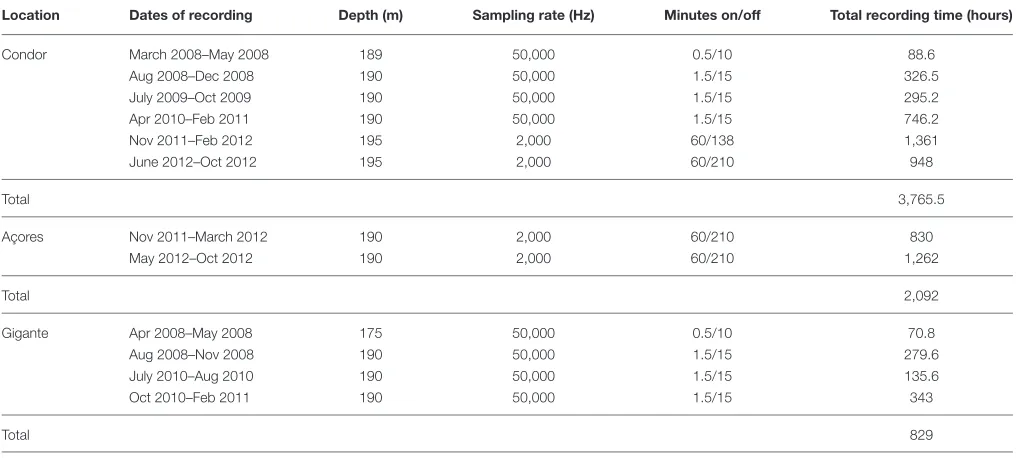
EARs recorded from March 2008 to October 2012 at Condor, from November 2011 to October 2012 at Açores and from April 2008 to February 2011 at Gigante with several gaps due to equipment failure or maintenance duties. Sampling rates and duty cycles were constrained by battery life and disk space limitations, given programmed deployment durations (Table 1).
Noise Measurements
Recordings with sample rates of 50 kHz were re-sampled to 2 kHz using Adobe Audition 3.0 software (Adobe Systems Incorporated, CA, USA) to standardize all acoustic data from 18 to 1,000 Hz, which is the bandwidth dominated by anthropogenic noise (Wenz, 1962) and overlaps the vocalizing range of balaenopterids. Self-system tonal noise within the frequency band of interest was identified only in recordings with sampling rates of 2,000 Hz which correspond to deployments at Condor and Açores from 2011 and 2012. 1-Hz Spectrogram Power Density (SPD) plots were made for each month to precisely identify which frequency bins were affected so they could be removed before computing broadband SPLs. Given that all self-system noise identified was highly tonal, removing these few frequency bins is likely to have a negligible effect on averaged broadband SPLs and on the characterization of shipping noise, which spreads across a wide range of frequencies. Moreover, self-system noise removed was found in frequencies well above the one-third octave bands analyzed in this study (63 and 125 Hz). From the SPD plots we can say that data were not clipped since there is no flat line of data points at high noise levels clustered at the limit value of 146 dB where the system saturates (see Figure 4 from results section).
Each month of recordings was grouped and concatenated to form a single file to be analyzed with Matlab code written byMerchant et al. (2015). The time-series of every signal was divided intom1-s segments of consecutive samples overlapping in time (50% overlap). Each segment was then multiplied by a Hann window and transformed to the frequency domain via the Discrete Fourier Transform (DFT). Spectra were then averaged to a 90-s resolution via the standard Welch method (Welch, 1976). The power spectrum (P) was then computed from the DFT, which for themthsegment, of signal X at frequencyf and for N number of samples in each segment is given by:
P(m) f =
Xm(f)
N 2
For each deployment, calibration data from the EAR, including the hydrophone sensitivity (Mh), system gain (G) and the zero-to-peak voltage of the analog-to-digital converter (VADC), were used to calculate a correction factor (S(f)) computed by:
S f
=Mh+G f
+20log10
1
VADC
+20log10 2Nbit−1
where Nbitis the bit-depth of the digital signal (16 bits). S(f) was then used to obtain SPLs in the bandwidth from 18 to 1,000 Hz by:
SPL(m)=10log10
1
Pref2
f′=fhigh
X
f′=flow
P(m)(f′)
B
−S
wherepref is the reference pressure of 1 µPa for underwater
measurements, flowand fhighare the lower and upper bounds of the frequency range under consideration and B is the noise power bandwidth of the window function, which corrects for the energy added through spectral leakage.
Noise Data Analysis
The effect of different duty cycles on the calculation of monthly average background noise levels was investigated by concatenating a full month of data (May 2008 from Condor), treating it as a continuous recording, and then subsampling it according to the different duty cycles used in this study (Table 1). To test for statistical differences in SPLs between different duty cycles, a first order autoregressive model was fitted to the SPL time series of mean SPL per sample for each duty cycle. Then, based on the estimated parameters and corresponding standard errors, 95% confidence intervals for each duty cycle mean SPLs were derived, assuming a Gaussian distribution for the parameter estimates. Number of samples (N) was the number of files resulting from the different duty cycles applied.
FIGURE 1 | Ecological Acoustic Recorders (EARs) deployment locations in the Azores archipelago (black dots).
TABLE 1 | Summary of acoustic data used in this work including recording dates, deployment depth, sampling rate, duty cycle, and total recording time.
Location Dates of recording Depth (m) Sampling rate (Hz) Minutes on/off Total recording time (hours)
Condor March 2008–May 2008 189 50,000 0.5/10 88.6
Aug 2008–Dec 2008 190 50,000 1.5/15 326.5
July 2009–Oct 2009 190 50,000 1.5/15 295.2
Apr 2010–Feb 2011 190 50,000 1.5/15 746.2
Nov 2011–Feb 2012 195 2,000 60/138 1,361
June 2012–Oct 2012 195 2,000 60/210 948
Total 3,765.5
Açores Nov 2011–March 2012 190 2,000 60/210 830
May 2012–Oct 2012 190 2,000 60/210 1,262
Total 2,092
Gigante Apr 2008–May 2008 175 50,000 0.5/10 70.8
Aug 2008–Nov 2008 190 50,000 1.5/15 279.6
July 2010–Aug 2010 190 50,000 1.5/15 135.6
Oct 2010–Feb 2011 190 50,000 1.5/15 343
Total 829
period considered was calculated. For N samples p2rms, AM is given by:
AM=10log10 1 N
PN
i=1p2rms,i
p2ref
!
wherep2rms,iis theith value of the mean squared pressure given by:
p2rms= f′=fhigh
X
f′=flow
P(m)(f′)
[image:4.595.44.552.410.639.2]To test for statistical differences in SPLs between locations, a first order autoregressive model was fitted to the SPL time series of each location (containing daily averaged SPLs). Then, based on the estimated parameters and corresponding standard errors, confidence intervals (95%CI) for each location mean SPLs were derived, assuming a Gaussian distribution for the parameter estimates. Number of samples (N) was the number of days.
Variability in noise levels for every location was analyzed using the coefficient of variation (CV), which allows comparison between datasets with different means.
Within each location, temporal variability of noise levels was explored by calculating hourly and monthly averaged, median and 5th, 75th, and 95th percentiles SPLs for the frequency band of 18–1,000 Hz. Also, hourly and monthly averaged one-third octave bands centered in 63 and 125 Hz were calculated to specifically measure the contribution of distant ship noise to ambient noise as suggested by the MSFD (2008/56/EC, European Commission 2008).
Seasons were defined according to the location (North-East Atlantic) as follows: Spring: March–May, Summer: June–August, Autumn: September–November and Winter: December–February.
To allow for comparisons, average SPLs were calculated for the three noisiest months in Condor (July-September, 2010), Açores (May-July, 2011) and Gigante (May–September, 2008) in the frequency band of 10–585 Hz to be compared to SPLs found in the Mediterranean byCastellote et al. (2012). Also, median levels in the frequency band of 10–25,000 Hz were measured in Condor (July-September, 2010) to compare it with levels found in another oceanic archipelago byBittencourt et al. (2016).
Ship Noise Analysis
In the absence of an operative antenna in the area for receiving information from Automatic Information System (AIS) installed in ships during the recording period, a methodology was used to study the contribution of local ship noise to general background noise levels. Using the broadband (18–1,000 Hz) noise background levels for every recording, an Adaptive Threshold Level (ATL;Merchant et al., 2012b) was obtained to identify local intermittent ship noise. The ATL was calculated by computing the minimum SPL in a certain period of time (W) and summing a tolerance above this minimum, a threshold ceiling (C) in dB re 1µPa:
ATL(t)=min[SPL(t)]t+W2
t−w2 +C
Due to differences in background noise levels and duty cycles in this study compared withMerchant et al. (2012b), two different periods of time (W) (1 and 7 hours of recordings) and 4 different threshold ceilings (C) (from 4, 6, 8, and to 12 dB) were tested. Firstly, an appropriate time period,W, was selected by visually inspecting plots of SPL values and thresholds and selecting the one that best discriminated wind-wave driven noise from intermittent noise. Once W had been specified, results from the ATL applying different values of C were compared to visually confirmed boats in the spectrogram for one chosen month per location (July 2012 for Condor, May 2012 for Açores
and July 2010 for Gigante). Those parameters that resulted in the best compromise between visually confirmed boats detected by the ATL (true positives) and detections by the ATL not corresponding to boats (false positives) were selected.
Once W and C were set, ATL was calculated for every month and location. Time with levels above the threshold was summed and divided by the total recording time to obtain the Percentage of Time with noise levels Above the Threshold Level (PT-ATL). The PT-ATL was then used to investigate spatial variations in boat presence using a Kruskal-Wallis ANOVA and apost-hocDunn test for multiple comparisons.
To test the efficiency of the methodology at detecting the presence of vessels, a comparison was made between monthly PT-ATLs and the number of days per month with boat presence in Condor. Data on boat presence were obtained from logbooks that contained information on the number of boats and type of activity conducted at the Condor seamount area per day from 2008 to 2012. The type of boats’ activities recorded were: recreational activities, such as big-game fishing and shark diving, with data logged by the operators themselves; scientific research, based on information provided by scientists conducting research at Condor; and tuna fishing, based on data recorded by onboard observers under the Azorean Fisheries Observer Programme (POPA).
Contribution of Wind-Wave and
Vessel-Driven Noise
An analysis of wind-wave driven noise and intermittent ship noise was implemented to compare the relative contribution of natural and anthropogenic sources to background noise levels in this region. Windiest months were selected for the three locations and daily averaged SPLs and wind speeds calculated. Days with maximum and minimum SPLs coincided with maximum and minimum wind speeds. For every month, averaged SPLs were calculated from 10 min sound files free of ship noise (visually inspected spectrograms) selected from 2 days, one with maximum and one with minimum wind speed. Similarly, for all months and for all locations, average SPLs were calculated for periods of time above the threshold and compared to those with minimum wind conditions. Differences between quietest average and noisiest average were then calculated for the wind and for the ship contribution. Daily averaged wind speeds (km/s) were obtained from Weather Underground historical data (www.wunderground.com) for each location.
Noise Levels above 120 dB re 1
µ
Pa
Since baleen whales have been shown to avoid vessels at noise levels above 120 dB re 1µPa (Richardson et al., 1995; Richardson
and Würsig, 1997; Southall et al., 2007), percentage of time with SPL above this level was also calculated for every month of study. To do so, broadband average SPL for every month and location were used to calculate the amount of time with noise levels above 120 dB re 1µPa and divide that by total recording
RESULTS
Ship Noise Analysis
The only anthropogenic noise source found in the recordings was ship noise, which had the maximum energy above 100 Hz for boats with higher noise levels, or in the bandwidth of 10–100 Hz for boats with lower noise levels.
The ATL only detected local boat noise that increased noise levels significantly and intermittently (Figure 2). The most adequate time period (W) to calculate minimum SPLs was 1 h of recordings for both duty cycles as this discriminated well between wind-driven and intermittent noise. The best compromise considering a minimum of 90% of visually confirmed boats in the spectrogram detected by the ATL, and a maximum of 5% of false positives was obtained using a threshold ceilingC=4 dB for duty cycle of 3,600 s every 12,600 s, andC=8 dB for the 90 and 30 s duty cycle (Table 2). False positives were mainly caused by loud biological sounds consisting of low frequency clicks produced by delphinids and sperm whales.
Logbook data from Condor was compared to the acoustic recordings resulting in 19 months of simultaneous data. There was a weak correlation (R2=0.354,p<0.05,n=19) between boat presence from logbooks and PT-ATL from 2008 to 2012, mainly because the high peak in PT-ATL in June was not matched
by a higher presence of boats (Figure 3). Removing June 2012 from the analysis resulted in a stronger correlation (R2=0.582,
p<0.001,n=18). Recordings from this month were visually inspected and boat noise detected by the ATL was confirmed to be mainly present during daylight hours.
Spatial Variability in Ambient Noise Levels
and Peak-Generating Vessels
The different duty cycles used in this study did not significantly affect the average monthly SPLs. Differences between the assumed “continuous” recording (AM=91.8, 95%CI=91.78– 91.82) and the different duty cycles were very small (1.5/15: AM
= 91.9, 95%CI= 91.72–92.02; 0.5/10: AM = 91.6, 95%CI =
91.45–91.62; 60/138: AM=91.4, 95%CI=91.40–91.47; 60/210:
AM=91, 95%CI=90.99–91.08), as were differences between
duty cycles. Therefore, comparison of noise levels between deployments and locations with different duty cycles should remain valid.
The arithmetic mean of SPLs was calculated for the 18–1,000 Hz band for Condor, Açores and Gigante over 9, 11, and 14 months, respectively. Açores had the lowest value (92.9 dB re 1
µPa), followed by Gigante (95.9 dB re 1µPa), with higher mean
[image:6.595.47.551.349.672.2]SPL in Condor (97.6 dB re 1µPa). Higher variability was found
TABLE 2 | Percentages of True Positives (TP), False Positives (FP), and False Negatives (FN) resulting from the comparison between boat detections applying the ATL function with different threshold ceilings (C) and visually confirmed boats in the spectrogram.
Threshold ceilings (dB) CONDOR AÇORES GIGANTE
TP FP FN TP FP FN TP FP FN
4 98.3 11.1 1.6 91.3 4.6 8.7 97.2 8.7 2.8
6 95.9 8.5 4.1 82.6 3.4 17.4 95.3 5.6 4.7
8 90.9 4.5 9.1 69.6 2.3 30.4 90.6 4 9.4
10 81 2.8 19 56.5 2.2 43.5 72.6 4.5 27.4
12 74.4 3.1 25.6 45.6 0 54.4 58.5 4.5 41.5
[image:7.595.45.293.222.353.2]Results are for July 2012 in Condor, May 2012 in Açores, and July 2010 in Gigante.
FIGURE 3 | Number of days with boats registered in logbooks (bars) and PT-ATL from the acoustic data (red line).
in Condor (CV=0.098) followed by Gigante (CV=0.085) and Açores (CV=0.071). Median values of noise levels were higher for Condor and Gigante (93.1dB re 1µPa and 91.6 dB re 1µPa,
respectively) and lower for Açores (90.1 dB re 1µPa). Averaged
noise levels for the 63 and 125 Hz one-third octave bands were also lower in Açores (70.2 dB re 1µPa and 74.6 dB re 1µPa,
respectively), while the highest levels at the 63 Hz band were found in Gigante (73.6 dB re 1µPa) and for the 125 Hz band
in Condor (79.5 dB re 1µPa;Table 3). There was no overlap in
the 95%CI of SPL within the 18–1,000 Hz, the 63 Hz and the 125 Hz one-third octave bands for Condor, Açores and Gigante, suggesting differences in average ambient noise levels between the three locations were highly significant (see Supplementary Table 1 for details on 95%CI values).
Differences in average noise levels for the 63 and 125 Hz one-third octave bands are supported by the spectral characteristics of sound for every location. Looking at the noisiest months, we can see that Gigante showed higher levels of noise from ships<100 Hz (Figure 4C) while Condor and Açores had higher ship noise levels>100 Hz (Figures 4A,B).
PT-ATL averaged across the same months showed that Gigante had the highest percentage of boat noise followed by Condor and Açores (Table 3). However, Condor showed a much higher variability (CV= 0.97) than Açores (CV =0.4) and Gigante (CV = 0.3). PT-ATLs differed between locations (Kruskal-Wallis H = 13.806, df = 2, p < 0.01) but only
TABLE 3 | Arithmetic mean (AM) (±SD) and median SPL at broadband levels (18–1,000 Hz) and one-third octave bands 63 and 125 Hz, and total PT-ATL for Condor, Açores and Gigante calculated over 9, 11, and 14 months, respectively.
Location Broadband noise levels (1–1,000 Hz)
63 Hz 125 Hz PT-ATL (%)
AM±SD Median AM±SD AM±SD Total
Condor 97.6±8.5 93.1 72.4±5.6 79.5±10.2 4.5
Açores 92.9±6.6 90.1 70.2±9.2 74.6±9.8 1.9
Gigante 95.9±8.2 91.6 73.6±12.8 76.0±11 6.0
differences between Gigante and Açores (p<0.001) and Gigante and Condor (p<0.05) were statistically significant.
Temporal Variability in Ambient Noise
Levels and Peak-Generating Vessels
In Condor seamount, percentage of time with boats peaked during the summer months (June–August) extending to September in some years (Figure 5D). This is well illustrated by increased broadband and 125 Hz octave band noise levels at these periods (Figures 5A,C). Açores seamount also showed higher PTL-ATL during summer months, especially in June, with another peak seen in November (Figure 6D). These peaks are well reflected in the higher average broadband and 63 and 125 Hz octave band noise levels (Figures 6A,C). In Gigante, values of PTL-ATL tended to be greater in summer months or in September, although differences to other seasons were not as obvious as in Condor and Açores (Figure 6D). In this case, temporal patterns in broadband and one-third octave bands SPLs did not match those of boat time (Figures 6A,C,D).
[image:7.595.303.553.270.356.2]FIGURE 4 | Spectrograms composed of PSDs with 1-s time segments (left) and spectral probability densities (SPDs), percentiles and root-mean-square (RMS) level (right) of 1 month of recordings for (A)Condor;(B)Açores; and(C)Gigante.
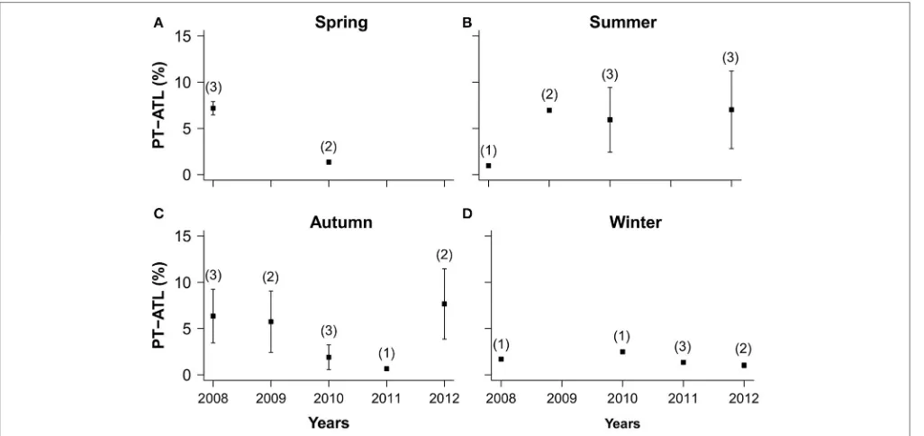
Annual trends in PT-ATL values for Condor averaged within seasons showed a decrease of boats from 2008 to 2010 in spring (Figure 7A), an increase between 2008 and 2010 in the summer (Figure 7B), a decrease from 2008 to 2011 and a subsequent increase in 2011 and 2012 in autumn (Figure 7C) and little variation over time in winter (Figure 7D).
Contribution of Wind-Wave and
Vessel-Driven Noise
A strong correlation was found between daily averaged noise levels and wind speed for the windiest months (November) in Condor (R2 = 0.8,p<0.001,n=30) and Açores (R2 =0.6,
p <0.001,n= 30) and a weak correlation for Gigante (R2 =
0.3,p<0.001,n=30). Average contribution of wind noise to background noise levels was of 10.8±3 dB in Condor (n=25), 7.7±2.5 dB in Açores (n=8) and 11.7±3.4 dB in Gigante (n=11).
Months with higher boat presence (August 2010 for Condor, June 2012 for Açores and August 2008 for Gigante) showed no or only a weak correlation between daily SPLs and wind speeds (Condor:R2=0.11,p=0.003,n=31; Açores:R2= −0.03,p=
0.9,n=30; Gigante:R2=0.06,p=0.1,n=26). In average, SPLs
for intermittent noise increased background noise levels in 19.3
±3.6 dB in Condor (n=32), 16.2±3 dB in Açores (n=11) and 18.3±3 dB in Gigante (n=14) with a maximum value of 29.1 dB for Condor in July of 2010.
Noise Levels above 120 dB re 1
µ
Pa
Percentage of time with noise levels>120 dB re 1µPa was higher
FIGURE 5 | Condor seamount: (A)hourly (gray lines) and monthly averages (red lines), medians (black lines) and 5th, 75th, and 95th percentiles (dashed black lines from bottom to top) SPLs in the 18–1,000 Hz frequency band.(B)monthly averaged wind speed (blue line).(C)hourly SPLs in the 63 Hz (dark gray lines) and 125 Hz (light gray lines) one-third octave bands and monthly averages (63 Hz: red line and 125 Hz: dashed red line).(D)monthly PT-ATL. Months are grouped in seasons below the x axis. Seasons are described as follows: SPR, Spring (March–May); SUM, Summer (June–August); AUT, Autumn (September–November) and WINT, Winter (December–February).
(0.03%) and June (0.07%) of 2012, while in Gigante, values>120 dB were recorded in 2008, with a maximum value of 0.12% in August, and in February 2011.
DISCUSSION
This work provides the first long-term characterization of low-frequency underwater noise levels at an important baleen whale mid-ocean habitat and discusses potential adverse effects on this cetacean group.
Noise levels at Condor seamount were higher than at Gigante and Açores seamounts and rises in monthly average broadband noise levels were mainly due to the presence of intermittent loud events such as boats. Median noise levels were more affected by wind-driven noise. In the absence of boats or with few boats, median and average levels were similar and wind became a major contributor to background noise.
The ATL methodology developed byMerchant et al. (2012b); to detect intermittent loud noise events attributed to boat presence has been successfully tested and applied in this study. Time period (W) over which minimum SPLs are calculated and threshold ceiling (C) are parameters that need readjustment depending on environmental acoustic characteristics and system duty cycle. We found that increasing C caused a decrease on the percentage of true and false positives but the extent of this
variation differed between locations, depending on the acoustic characteristics of the environment. In our case, the same W worked well for all duty cycles but the adequate threshold ceiling was lower for higher duty cycles than for lower duty cycles (Table 2). In general, environments with a high presence of loud intermittent events and systems with lower duty cycles should require smaller W and higher C than quieter places and higher duty cycles in order to detect these events above minimum SPLs. The high correlation between boat presence at Condor seamount from logbook data and PT-ATL values from 2009 to 2011 indicates that this methodology can be used to describe boat presence in the study area. The lack of correlation in 2012 is likely explained by the limitations in boat detection distance using these methods and the fact that not all boat activity was registered in logbooks. We suspect that the high PT-ATL values found in June 2012 could be due to an increase in recreational activities.
FIGURE 6 | Açores and Gigante seamount: (A)hourly (gray lines) and monthly averages (red lines), medians (black lines) and 5th, 75th, and 95th percentiles (dashed black lines from bottom to top) SPLs in the 1–1,000 Hz frequency band.(B)monthly averaged wind speed (blue line).(C)hourly SPLs in the 63 Hz (light gray lines) and 125 Hz (dark gray lines) one-third octave bands and monthly averages (63 Hz: red line and 125 Hz: dashed red line).(D)monthly PT-ATL. Months are grouped in seasons below the x axis. Seasons are described as follows: SPR, Spring (March–May); SUM, Summer (June–August); AUT, Autumn
(September–November) and WINT, Winter (December–February).
experimentally in 2009 and that mostly operate in spring and summer (Ressurreição and Giacomello, 2013). The expeditions to dive with sharks at Condor were reported to double between 2011 and 2012 (Ressurreição and Giacomello, 2013), which might well explain why PT-ATL values increased in 2012. This activity also takes place in the Açores seamount, but to a lesser extent, which is reflected by a lower boat presence than in Condor. Gigante seamount shows a higher presence of boats throughout the year, as a result of the proximity of a marine traffic route used by commercial shipping and the presence of commercial fishing year-round in Gigante. Therefore, there is a great potential for using passive acoustic techniques to monitor boat activity in specific areas such as the ones in the study. This methodology, however, cannot be used to detect distant vessels and might not be adequate for areas with higher ship traffic where separation between continuous and intermittent events might not be possible.
For measuring the contribution of distant ship noise, the European MSFD (2008/56/EC, European Commission 2008) suggests the use of one-third octave bands, centered at 63 Hz and 125 Hz, which are included as indicators to assess the Good Environmental Status (GES) of the marine environment. In this study, Gigante shows the highest noise levels in the 63 Hz one-third octave band which can be explained by the proximity of a shipping lane mentioned in the above paragraph. Noise levels
measured in the 125 Hz octave band better reflect local boat presence at Condor and Açores while at Gigante the difference between the two octave bands (63 and 125 Hz) is not very clear. This is mainly due to the difference in the type of vessels and distance of those to the hydrophone at each location. Comparison of spectrum levels indicates that Gigante has higher noise levels below 100 Hz, which is typical of distant large vessels such as tankers, while Condor and Açores have higher levels above 100 Hz, which is characteristic of smaller boats. Performance of one-third octave bands with distant shipping could not be assessed in this study because AIS data were not available for this period.
FIGURE 7 | Inter-annual variability in averaged seasonal PT-ATL values for Condor seamount and standard deviations (error bars).Numbers in brackets are number of months with data representing each of the following seasons:(A)Spring: March–June;(B)Summer: June–September;(C)Autumn:
October–November;(D)Winter: December–February.
in response to shipping noise. Blue whales have been found to change the interval, types and amplitudes of their calls (McKenna, 2011; Melcón et al., 2012) while male fin whales seem to change their song characteristics (Castellote et al., 2012). Other baleen whale species such as gray whales (Eschrichtius robustus) also modify calling rates, received levels and percentage of calls (Dahlheim and Castellote, 2016), humpback whales sing shorter versions of their songs (Sousa-Lima et al., 2002) and North Atlantic right whales show short- and long-term changes in their calling behavior in response to increased low-frequency noise (Parks et al., 2007, 2009, 2010). However, other studies show that humpback whales respond to increases of noise levels produced by wind but do not compensate for higher levels of noise from vessels (Dunlop, 2016).
Auditory masking reduces the effective communication space between sender and receiver (Clark et al., 2009). A model developed byTennessen and Parks (2016)demonstrated that a right whale is not able to hear an upcall from another whale if a ship passes at less than 25 Km, unless the calling whale increases the amplitude of the calls by 20 dB. Despite differences in call source levels between right whales and blue, fin and sei whales, they share similarities in call frequency ranges (e.g.,Parks and Tyack, 2005; Sirovi´c et al., 2007; Romagosa et al., 2015). Detection ranges of calls for these three species might be affected by passing ships in similar ways, which is of concern given the dependence of Balaenoperids on long range communication (Payne and Webb, 1971). Although their calls have been mainly attributed to male reproductive displays, whales also produce sounds outside their breeding grounds and season (Clark et al., 2002; Oleson et al., 2007; Vu et al., 2012). Blue whales are known to produce D calls
during foraging within groups (McDonald et al., 2001; Stafford et al., 2005; Calambokidis et al., 2008) and fin whales produce “20-Hz pulse” calls that are likely to have a social purpose or a contact maintaining function when produced irregularly or as call-counter calls (McDonald et al., 1995; Edds-Walton, 1997). Baleen whale long-range calls could also be used for orientation purposes, as suggested byPayne and Webb (1971). In the Azores, preliminary analysis of acoustic data shows that blue and fin whales produce these types of calls when they are seen in spring as well as reproductive songs during the winter (unpublished data). Sei whales also vocalize during their migratory journey (Olsen et al., 2009; Prieto et al., 2014) through the Azores producing a well-known downsweep call for this species (Romagosa et al., 2015). Several studies indicate that blue, fin and sei whales are present around the archipelago, including in the deployment areas, mostly from February to May (Silva et al., 2014; Prieto et al., in press) which coincides with a lower presence of boats at Condor but with a higher presence of boats at Açores. As for the transiting area (Gigante), due to its more constant vessel traffic throughout the year, an overlap exists with the baleen whale northward migration in spring and summer, and possibly with the southward journey in late autumn.
been made to develop masking models that can be incorporated into regulation strategies, more research is needed to better understand potential effects of this complex phenomena, hearing characteristics from different species and anti-masking strategies used by free-ranging animals (Erbe, 2002; Clark et al., 2009).
Ship noise can also cause behavioral responses to cetaceans and Southall et al. (2007) suggests using SPLs to assess it. This metric might not be the most appropriate way to look for consistent patterns of response but it is often measured or estimated because it is required by law in many European countries and the USA as part of their noise mitigation regulations. Also, many other variables such as location, nature and behavior of noise sources and characteristics and activity of the individual animal among others, can affect the nature and extent of responses (Ellison et al., 2012). Therefore, the percentage of time with SPL levels above 120 dB re 1 µPa
was calculated based on the model from theNRC (2005) that established that marine mammals exposed to levels above this value might be affected by sound. The maximum monthly percentage time with levels above 120 dB re 1µPa was 3.3% (at
Condor seamount) which is very low considering that an animal is unlikely to remain in the same location for the entire month. However, deployment depth affect noise levels received by the hydrophone and percentages with levels above 120 dB re 1µPa
are certainly higher closer to the source which in this case is found at the surface. While this is a simplistic and limited approach, it can nevertheless give an initial sense of the time that noise levels in an area could induce behavioral responses on baleen whales.
Comparatively, average noise levels for the three noisiest months at Condor (100.1±17.2 dB re 1µPa), Açores (95.9±
7 dB re 1 µPa) and Gigante (96.2± 13 dB re 1µPa) for the
frequency band of 10–585 Hz are lower than those measured byCastellote et al. (2012)in areas of the Mediterranean, such as the Provençal (106.9 ± 5.3 dB re 1 µPa), Alboran (103.7 ± 2.5 dB re 1 µPa) and Balearic (105.2 ± 1.2 dB re 1 µPa)
basins and the Strait of Gibraltar (112.5±4 dB re 1µPa). Also,
median noise levels within the 10–25,000 Hz measured in winter at Trindade-Martin Vaz Archipelago (113.7±11.4 dB re 1µPa),
another oceanic archipelago in the Southwestern Atlantic, are higher than those of Condor (105.3±11.4 dB re 1µPa) for the
same frequency band (Bittencourt et al., 2016). Differences in this case might be explained by presence of snapping shrimp found to be an important noise contributor in shallow waters (Hildebrand, 2009).
Despite our findings suggesting the Azores is characterized by reduced underwater noise, we expect other areas in the archipelago closer to ferry routes, commercial shipping routes or routinely used by whale watching boats to be considerably noisier. Therefore, these measurements are representative only of these locations and further measurements and sound
propagation modeling in other areas will be necessary to produce a detailed soundscape for the entire archipelago.
AUTHOR CONTRIBUTIONS
Conceived and designed the work: MR and MS. Collected the data: IC, ML, EG, and MS. Performed data analysis and interpretation: MR, NM, EG, TM, and MS. Wrote the paper: MR. Reviewed the manuscript and approved the final version; MR, IC, NM, ML, EG, TM, and MS.
FUNDING
Fundação para a Ciência e a Tecnologia (FCT) and Fundo Regional da Ciência e Tecnologia (FRCT), through research projects TRACE (PTDC/MAR/74071/2006), MAPCET (M2.1.2/F/012/2011), and FCT Exploratory project (IF/00943/2013/CP1199/CT0001), supported by funds from FEDER, the Competitiveness Factors Operational (COMPETE), QREN, POPH, European Social Fund, Portuguese Ministry for Science and Education, and Proconvergencia Açores/EU Program. We also acknowledge funds provided by FCT to MARE, through the strategic project UID/MAR/04292/2013, that also supported fees for this open access publication. MR is supported by a DRCT doctoral grant (M3.1.a/F/028/2015), IC was supported by a FCT doctoral grant (SFRH/BD/41192/2007) and MAS is supported by an FCT-Investigator contract (IF/00943/2013). TM is a member of CEA/UL (Funded by FCT - Fundação para a Ciência e a Tecnologia, Portugal, through the project UID/MAT/00006/2013).
ACKNOWLEDGMENTS
We are grateful to Rui Prieto, the skippers and crew members that helped with the deployment of the EARs. Data on boat presence were kindly provided by the Azores Fisheries Observer Program (POPA) (www.popaobserver.org) and by tourism operators (in the latter case an output of the projects CONDOR (EEA Grants PT-0040/2008) and SMaRT (M.2.1.2/029/2011)). We are also grateful to Ricardo Serrão Santos for his support and useful comments. Comments and suggestions from two reviewers significantly improved the present paper. This work is an output of research projects TRACE-PTDC/MAR/74071/2006, MAPCET-M2.1.2/F/012/2011, and of the FCT-Exploratory project IF/00943/2013/CP1199/CT0001.
SUPPLEMENTARY MATERIAL
The Supplementary Material for this article can be found online at: http://journal.frontiersin.org/article/10.3389/fmars. 2017.00109/full#supplementary-material
REFERENCES
Andrew, R. K., Howe, B. M., Mercer, J. A., and Dzieciuch, M. A. (2002). Ocean ambient sound: comparing the 1960s with the 1990s for a receiver off the California coast.Acoust. Res. Lett. Online3, 65–70. doi: 10.1121/1.1461915
Bassett, C., Polagye, B., Holt, M. M., and Thomson, J. (2012). A vessel noise budget for Admiralty Inlet, Puget Sound, Washington (USA).J. Acoust. Soc. Am.132, 3706–3719. doi: 10.1121/1.4763548
Sea Res. I Oceanogr. Res. Papers 115, 103–111. doi: 10.1016/j.dsr.2016. 06.001
Blair, H. B., Merchant, N. D., Friedlaender, A. S., Wiley, D. N., and Parks, S. E. (2016). Evidence for ship noise impacts on humpback whale foraging behaviour.Biol. Lett.12:20160005. doi: 10.1098/rsbl.2016.0005
Calambokidis, J., Schorr, G. S., Steiger, G. H., Francis, J., Bakhtiari, M., Marshall, G., et al. (2008). Insights into the underwater diving, feeding, and calling behavior of blue whales from a suction-cup-attached video-imaging tag (CRITTERCAM). Mar. Technol. Soc. J. 41, 19–29. doi: 10.4031/002533207787441980
Castellote, M., Clark, C. W., and Lammers, M. O. (2012). Acoustic and behavioural changes by fin whales (Balaenoptera physalus) in response to shipping and airgun noise.Biol. Conserv.147, 115–122. doi: 10.1016/j.biocon.2011.12.021 Chapman, N. R., and Price, A. (2011). Low frequency deep ocean ambient noise
trend in the Northeast Pacific Ocean.J. Acoust. Soc. Am.129, E161–E165. doi: 10.1121/1.3567084
Clark, C. W., Borsani, F., and Notarbartolo di Sciara, G. (2002). Vocal activity of fin whales,Balaenoptera physalus, in the Ligurian Sea.Mar. Mam. Sci.18, 281–285. doi: 10.1111/j.1748-7692.2002.tb01035.x
Clark, C. W., Ellison, W. T., Southall, B. L., Hatch, L., Van Parijs, S. M., Frankel, A., et al. (2009). Acoustic masking in marine ecosystems: intuitions, analysis, and implication.Mar. Ecol. Prog. Ser.395, 201–222. doi: 10.3354/meps 08402
Dahlheim, M., and Castellote, M. (2016). Changes in the acoustic behavior of gray whalesEschrichtius robustusin response to noise.Endang. Species Res.31, 227–242. doi: 10.3354/esr00759
Di Ioro, L., and Clark, C. W. (2010). Exposure to seismic survey alters blue acoustic communication.Biol. Lett.5, 51–54. doi: 10.1098/rsbl.2009.0651
Dudzinski, K. A., Thomas, J. A., and Douaze, E. (2002). “Communication,” in
Encyclopedia of Marine Mammals,eds W. F. Perrin, B. Wursig, and J. G. M. Thewissen (San Diego, CA: Academic Press), 248–268.
Dunlop, R. (2016). The effect of vessel noise on humpback whale,Megaptera novaeangliae, communication behavior. Anim. Behav. 111, 13–21. doi: 10.1016/j.anbehav.2015.10.002
Dziak, R. P., Bohnenstiehl, D. R., Stafford, K. M., Matsumoto, H., Park, M., Lee, W. S., et al. (2015). Sources and levels of ambient ocean sound near the Antarctic Peninsula.PLoS ONE10:e0123425. doi: 10.1371/journal.pone.01 23425
Edds-Walton, P. L. (1997). Acoustic communication signals of mysticete whales.
Bioacoustics8, 47–60. doi: 10.1080/09524622.1997.9753353
Ellison, W. T., Southall, B. L., Clark, C. W., and Frankel, A. S. (2012). A new context-based approach to assess marine mammal behavioral responses to anthropogenic sounds.Conserv. Biol.26, 21–28. doi: 10.1111/j.1523-1739.2011. 01803.x
Erbe, C. (2002). Underwater noise of whale-watching boats and potential effects on killer whalesOrcinus orca, based on an acoustic impact model.Mar. Mam. Sci.
18, 394–418. doi: 10.1111/j.1748-7692.2002.tb01045.x
Erbe, C., Reichmuth, C., Cunningham, K., Lucke, K., and Dooling, R. (2015). Communication masking in marine mammals: a review and research strategy.
Mar. Pollut. Bull.103, 15–38. doi: 10.1016/j.marpolbul.2015.12.007
Giacomello, E., Menezes, G. M., and Bergstad, O. A. (2013). An integrated approach for studying seamounts: CONDOR observatory. Deep Sea Res. Part II Top. Stud. Oceanogr 98, 1–6. doi: 10.1016/j.dsr2.2013. 09.023
Hatch, L. T., Clark, C. W., Van Parijs, S. M., Frankel, A. S., and Ponirakis, D. W. (2012). Quantifying loss of acoustic communication space for right whales in and around a U.S. national marine sanctuary.Conserv. Biol.26, 983–994. doi: 10.1111/j.1523-1739.2012.01908.x
Hildebrand, J. A. (2009). Anthropogenic and natural sources of ambient noise in the ocean.Mar. Ecol. Prog. Ser.395, 5–20. doi: 10.3354/meps08353
Klinck, H., Nieukirk, S. L., Mellinger, D. K., Klinck, K., Matsumoto, H., and Dziak, R. P. (2012). Seasonal presence of cetaceans and ambient noise levels in polar waters of the North Atlantic.J. Acoust. Soc. Am.132, EL176–EL181. doi: 10.1121/1.4740226
Lammers, M. O., Brainard, R. E., Au, W. W. L., Mooney, T. A., and Wong, K. B. (2008). An Ecological Acoustic Recorder (EAR) for long-term monitoring of biological and anthropogenic sounds on coral reefs and other marine habitats.
J. Acous. Soc. Am.123, 1720–1728. doi: 10.1121/1.2836780
Lombard, É. (1911). Le signe de l’élévation de la voix.Ann. Mal.L’Oreille Larynx
37, 101–109.
McDonald, M. A., Hildebrand, J. A., and Webb, S. C. (1995). Blue and fin whales observed on a seafloor array in the Northeast Pacific.J. Acoust. Soc. Am.98, 712–721. doi: 10.1121/1.413565
McDonald, M. A., Calambokidis, J., Teranishi, A. M., and Hildebrand, J. A. (2001). The acoustic calls of blue whales off California with gender data.J. Acoust. Soc. Am.109, 1728−1735. doi: 10.1121/1.1353593
McDonald, M. A., Hildebrand, J. A., and Wiggins, S. M. (2006). Increases in deep ocean ambient noise in the Northeast Pacific west of San Nicolas Island, California.J. Acoust. Soc. Am.120, 711–717. doi: 10.1121/1.2216565 McKenna, M. F. (2011). Blue Whale Response to Underwater Noise from
Commercial Ships. Ph.D. thesis in Oceanography at the University of California San Diego.
Melcón, M. L., Cummins, A. J., Kerosky, S. M., Roche, L. K., Wiggins, S. M., and Hildebrand, J. A. (2012). Blue whales respond to anthropogenic noise.PLoS ONE7:681. doi: 10.1371/journal.pone.0032681
Merchant, N. D., Blondel, P., Dakin, D. T., and Dorocicz, J. (2012a). Averaging underwater noise levels for environmental assessment of shipping.J. Acous. Soc. Am.132, EL343–EL349. doi: 10.1121/1.4754429
Merchant, N. D., Witt, M. J., Blondel, P., Godley, B. J., and Smith, G. H. (2012b). Assessing sound exposure from shipping in coastal waters using a single hydrophone and Automatic Identification System (AIS) data.Mar. Pollut. Bull.
64, 1320–1329. doi: 10.1016/j.marpolbul.2012.05.004
Merchant, N. D., Fristrup, K. M., Johnson, M. P., Tyack, P. L., Witt, M. J., Blondel, P., et al. (2015). Measuring acoustic habitats.Methods Ecol. Evol.6, 257–265. doi: 10.1111/2041-210X.12330
Miller, P. J. O., Biassoni, N., Samuels, A., and Tyack, P. L. (2000). Whale songs lengthen in response to sonar.Nature405, 903. doi: 10.1038/35016148 Nieukirk, S. L., Mellinger, D. K., Moore, S. E., Klinck, K., Dziak, R. P., and Goslin,
J. (2012). Low-frequency whale and seismic airgun sounds recorded in the mid-Atlantic Ocean.J. Acous. Soc. Am.115, 1832–1843. doi: 10.1121/1.1675816 NRC (2005).Marine Mammal Populations and Ocean Noise: Determining When Noise Causes Biologically Significant Effects. Washington, DC: The National Academies Press.
Olsen, E., Budgell, W. P., Head, E., Kleivane, L., Nøttestad, L., Prieto, R., et al. (2009). First satellite-tracked long-distance movement of a sei whale (Balaenoptera borealis) in the North Atlantic.Aquat. Mamm.35, 313–318. doi: 10.1578/AM.35.3.2009.313
Oleson, E. M., Calambokidis, J., Burgess, W. C., McDonald, M. A., LeDuc, C. A., and Hildebrand, J. A. (2007). Behavioral context of call production by eastern North Pacific blue whales.Mar. Ecol. Prog. Ser.330, 269−284. doi: 10.3354/meps330269
Parks, S. E., Clark, C. W., and Tyack, P. L. (2007). Short- and long-term changes in right whale calling behavior: the potential effects of noise on acoustic communication.J. Acoust. Soc. Am.122, 3725–3731. doi: 10.1121/1.2799904 Parks, S. E., Johnson, M., Nowacek, D., and Tyack, P. L. (2010). Individual
right whales call louder in increased environmental noise.Biol. Lett.7, 33–35. doi: 10.1098/rsbl.2010.0451
Parks, S. E., and Tyack, P. L. (2005). Sound production by North Atlantic right whales (Eubalaena glacialis) in surface active groups.J. Acoust. Soc. Am.117, 3297–3306.
Parks, S. E., Urazghildiiev, I., and Clark, C. W. (2009). Variability in ambient noise levels and call parameters of North Atlantic right whales in three habitat areas.
J. Acoust. Soc. Am.125, 1230–1239. doi: 10.1121/1.3050282
Payne, R., and Webb, D. (1971). Orientation by means of long range acoustic signaling in baleen whales. Ann. N.Y. Acad. Sci. 188, 110–142. doi: 10.1111/j.1749-6632.1971.tb13093.x
Ponce, D., Thode, A. M., Guerra, M., Urbán, R. J., and Swartz, S. (2012). Relationship between visual counts and call detection rates of gray whales (Eschrichtius robustus) in Laguna San Ignacio, Mexico.J. Acoust. Soc. Am.131, 2700–2713. doi: 10.1121/1.3689851
Prieto, R., Silva, M. A., Waring, G. T., and Gonçalves, J. M. A. (2014). Sei whale movements and behaviour in the North Atlantic inferred from satellite telemetry.Endanger. Species Res.26, 103–113. doi: 10.3354/esr00630 Prieto, R., Tobeña, M., and Silva, M. A. (in press). Habitat preferences of baleen
whales in a mid-latitude habitat.Deep Sea Res. Part II Top. Stud. Oceanogr.
Ressurreição, A., and Giacomello, E. (2013). Quantifying the direct use value of Condor seamount. Deep Sea Res. II 98, 209–217. doi: 10.1016/j.dsr2.2013.08.005
Richardson, W. J., and Würsig, B. (1997). Influences of man-made noise and other human actions on cetacean behaviour.Mar. Freshwater Behav. Physiol.
29, 183–209. doi: 10.1080/10236249709379006
Richardson, W. J., Greene, C. R. Jr., Malme, C. I., and Thomson, D. H. (1995).
Marine Mammals and Noise.San Diego, CA: Academic Press.
Rolland, R. M., Parks, S. E., Hunt, K. E., Castellote, M., Corkeron, P. J., Nowacek, D. P., et al. (2012). Evidence that ship noise increases stress in right whales.
Proc. R. Soc. B.279, 2363–2368. doi: 10.1098/rspb.2011.2429
Romagosa, M., Boisseau, O., Cucknell, A.-C., Moscrop, A., and McLanaghan, R. (2015). Source level estimates for sei whale (Balaenoptera borealis) vocalizations off the Azores.J. Acoust. Soc. Am.138, 2367–2372. doi: 10.1121/1.4930900 Ross, D. (1976).Mechanics of Underwater Noise.Oxford: Pergamon Press. Ross, D. (2005). Ship sources of ambient noise.IEEE J. Ocean. Eng.30, 257–261.
doi: 10.1109/JOE.2005.850879
Samaran, F., Adam, O., and Guinet, C. (2010). Detection range modeling of blue whale calls in Southwestern Indian Ocean.Appl. Acoust.71, 1099–1106. doi: 10.1016/j.apacoust.2010.05.014
Silva, M. A., Prieto, R., Cascão, I., Oliveira, C., Vaz, J., Lammers, M. O., et al. (2011). “Fin whale migration in the North Atlantic: placing the Azores into the big picture,” inAbstract Book of the 19th Biennial Conference on the Biology of Marine Mammals(Tampa, FL).
Silva, M. A., Prieto, R., Jonsen, I., Baumgartner, M. F., and Santos, R. S. (2013). North Atlantic blue and fin whales suspend their Spring migration to forage in middle latitudes: building up energy reserves for the journey?.PLoS ONE
8:e76507. doi: 10.1371/journal.pone.0076507
Silva, M. A., Prieto, R., Cascão, I., Seabra, M., I., Machete, M., Baumgartner, M. F. et al. (2014). Spatial and temporal distribution of cetaceans in the mid-Atlantic waters around the Azores. Mar. Biol. Res. 10, 123–137. doi: 10.1080/17451000.2013.793814
Sirovi´c, A., Hildebrand, J. A., and Wiggins, S. M. (2007). Blue and fin whale call source levels and propagation range in the Southern Ocean.J. Acoust. Soc. Am.
122, 1208–1215. doi: 10.1121/1.2749452
Širovi´c, A., Hildebrand, J., and McDonald, M. (2016). Ocean ambient sound south of Bermuda and Panama Canal traffic.J. Acoust. Soc. Am.139, 2417–2423. doi: 10.1121/1.4947517
Sousa-Lima, R. S., Morete, M. E., Fortes, R. C., Freitas, A. C., and Engel, M. H. (2002). Impact of boats on the vocal behavior of humpback whales off Brazil.J. Acoust. Soc. Am.112, 2430–2431. doi: 10.1121/1.4779974
Southall, B. L., Bowles, A. E., Ellison, W. T., Finneran, J. J., Gentry, R. L., Greene, C., et al. (2007). Marine mammal noise exposure criteria: initial scientific recommendations. Aquat. Mamm. 33, 411–521. doi: 10.1578/AM.33.4.20 07.411
Stafford, K. M., Moore, S. E., and Fox, C. G. (2005). Diel variation in blue whale calls recorded in the eastern tropical Pacific.Anim. Behav.69, 951–958. doi: 10.1016/j.anbehav.2004.06.025
Tennessen, J., and Parks, S. (2016). Acoustic propagation modeling indicates vocal compensation in noise improves communication range for North Atlantic right whales.Endanger. Species Res.30, 225–237. doi: 10.3354/esr00738
Vu, E., Risch, D., Clark, C., Gaylord, S., Hatch, L., Thompson, M., et al. (2012). Humpback whale song occurs extensively on feeding grounds in the western North Atlantic Ocean.Aquat. Biol.14, 175–183. doi: 10.3354/ ab00390
Welch, P. (1976). The use of fast Fourier transform for the estimation of power spectra: A method based on time averaging over short, modified periodograms.
IEEE Trans. Audio Electroacoust.15, 70–73. doi: 10.1109/TAU.1967.1161901 Wenz, G. M. (1962). Acoustic ambient noise in the ocean: Spectra and sources.J.
Acoust. Soc. Am.34, 1936–1956. doi: 10.1121/1.1909155
Williams, R., Wright, A. J., Ashe, E., Blight, L. K., Bruintjes, R., Canessa, R., et al. (2015). Impacts of anthropogenic noise on marine life: Publication patterns, new discoveries, and future directions in research and management.Ocean Coast. Manag.115, 17–24. doi: 10.1016/j.ocecoaman.2015.05.021
Conflict of Interest Statement: The authors declare that the research was conducted in the absence of any commercial or financial relationships that could be construed as a potential conflict of interest.