Robust audio sensing with multi sound classification

Robust Audio Sensing with Multi-Sound

Classification

Peter Haubrick and Juan Ye

School of Computer Science, University of St Andrews

St Andrews, UK [email protected]

Abstract—Audio data is a highly rich form of information, often containing patterns with unique acoustic signatures. In pervasive sensing environments, because of the empowered smart devices, we have witnessed an increasing research interest in sound sensing to detect ambient environment, recognise users’ daily activities, and infer their health conditions. However, the main challenge is that the real-world environment often contains multiple sound sources, which can significantly compromise the robustness of the above environment, event, and activity detection applications. In this paper, we explore different approaches in multi-sound classification, and propose a stacked classifier based on the recent advance in deep learning. We evaluate our proposed approach in a comprehensive set of experiments on both sound effect and real-world datasets. The results have demonstrated that our approach can robustly identify each sound category among mixed acoustic signals, without the need of any a priori knowledge about the number and signature of sounds in the mixed signals.

Index Terms—Acoustic sensing, multi-sound classification, en-semble classification, convolutional neural network

I. INTRODUCTION

Audio signal processing is attracting increasing attention as it has demonstrated its potential in detecting a wide range of events and activities. Audio sensing can contribute to daily activity recognition by detecting the use of appliances like coffee machine or microwave. It also helps to identify environmental context by detecting ambient sound [18].

Significant progress has made in sound event classification, as a large amount of research effort has been devoted to extracting various types of features in both time and frequency domains from audio signals and applying machine learning techniques in recognising the category for each sound event. The majority of existing work focuses on single sound event classification, or monophonic detection in the terminology of audio signal processing; i.e., classifying sound category in a single source environment [16]. However, rarely does a real-world environment contain only one sound source; for example, an office environment might mix sounds from keyboard typing, clearing throat, and door closing. To enable robust audio sensing, we need an algorithm that can accurately detect and classify each sound category from such mixed audio data; i.e.,polyphonic detection.

Polyphonic detection in unconstrained, real-world environ-ment is a challenging task. First of all, mixed sounds can drastically alter the acoustic signature, so features extracted from mixed audio data do not match with features from

individual sound. A traditional approach in audio signal pro-cessing is to separate sounds in the pre-propro-cessing stage; for example, identifying instruments in music [10]. However, it often requires pre-knowledge on the number of sounds being mixed and their individual signatures; e.g., frequency band. Recently, multi-label deep neural networks [1] and RNN [16] have achieved promising results in multi-sound classification. However, they require a large number of training data to learn complex patterns in mixed sounds.

In this paper, we present a novel hierarchical architecture to enable robust multi-sound classification with a priori knowl-edge of the number and profile of each mixed sound. We apply a state-of-the-art CNN pre-trained on AudioSet [9] to learn acoustic features, a binary classifier to characterise each sound category, and a stacked classifier to learn the outcome of each binary classifier for multi-sound classification. To reduce the burden of data collection and labelling, we will train our model on publicly available sound effect datasets. With appropriate data augmentations, these datasets have been demonstrated as an acceptable alternative for real-world audio data [12], [19]. Here, we will generate synthesised mixtures of sounds from the sound effect datasets, use them to train our model, and evaluate the trained model on the real-world dataset. This helps to assess to what degree we can rely on the synthesised sound data to recognise real-world audio recordings. To test the generalisation and robustness of our model, we conduct extensive experiments on systematically mixing similar and distinct sound classes.

The rest of the paper is organised as follows. Section II introduces the most relevant work in the literature and com-pares and contrasts with our approach. Section III explores different approaches in tackling multi-sound classification and introduces our final design of the algorithm. Section IV illustrates the evaluation methodology and analyse and discuss the results. Section V summarises the paper and point to the future directions.

II. RELATEDWORK

Mobile audio sensing enables to infer a wide range of daily activities, ambient conditions, and people’s affective states and health conditions.

One of the most common approaches in audio signal processing is to extract temporal and frequency domain features. MFCC has been popularly used in speech detection. Combining MFCC along non-speech data such as tone and pitch, verbal and visual cues, Lee et al. have designed a system to monitor face-to-face interaction in everyday, real-world situations [13]. Rachuri et al. [20] have extracted Perceptual Linear Predictive (PLP) coefficients and applied GMM to classify emotional states of a speaker.

B. Deep Neural Networks

Lane et al. [11] propose a mobile audio sensing framework, called DeepEar, on a coupled architecture of 4 deep neural networks (DNNs), corresponding to 4 audio categories, in-cluding ambient audio scene, speaker identification, emotion recognition, and stress detection. Our approach is similar to

DeepEar in that we also build on top of a CNN for acoustic

feature learning. The main difference is that DeepEar dedi-cates different CNNs for different types of sound detection, while we design a hierarchical architecture to enable multiple simultaneous sound event classification.

Laput et al. [12] present a real-time, sound-based activity recognition system, called Ubicoustics. It is trained on a collection of professional sound effect libraries that have been traditionally used in the entertainment industry. To tune the sound effect data towards audio samples to be collected in real-world environments, the authors have performed data augmentation including amplitude, reverb, and mixing. Similarly, Salamon and Bello have designed a set of deformations resulting augmentation, including time stretching, pitch shifting, dynamic range compression, and background noise [21]. These augmentations have significantly improved the classification accuracies on a range of environmental sound classification tasks, including air conditioner, car horn, dog barking, and siren. Our approach is similar to Ubicoustics in that we also use sound effect dataset for training the model and we are also borrowing state-of-the-art data augmentation techniques to enhance the generalisation and applicability of sound effect dataset in real-world sound classification. The major difference is that we design a stacked classifier on top of this basic approach to enable multi-sound classification.

C. Multi-Sound Separation

Sound source separation and classification under overlap-ping conditions has been one of the most challenging tasks in audio classification [2]. Tran and Li have used Jump Function Kolmogorov (JFK) to separate sound signal into each wavelet sub-band and then run binary SVM for classifying each sound event [23]. Park et al. have used NMF [8] with spectral enve-lope constraints to separate instrument sounds [17]. However, it requiresa prioriknowledge on mixed sound events, which can be impractical in real-world situations.

More recently, various deep learning techniques have been applied to multi-sound event detection [7], [16]. Cakir et al. propose multi-label convolutional recurrent neural

net-works [1], where CNN is used to extract higher level features through multiple convolutional layers and pooling in frequency domain, and then these features are fed to recurrent layers, whose features are used to obtain event probabilities through a feed-forward fully connected layer. Differently, our approach first trains binary classifiers to learn profiles for each sound category with the features produced from the CNN. Then it trains a stacked ensemble for multi-sound classification with mixed sound data by learning the correlations between binary classifiers’ probability distributions and multi-sound labels. The separation of single- and multi-sound training in different learning processes can reduce the burden on collecting and labelling multi-sound training data.

III. PROPOSEDAPPROACH

In this paper, we propose a novel stacked classifier to automatically classify and distinguish individual acoustic events from mixed audio data without any pre-knowledge on how many events are mixed and what signature of each sound exhibits (such as their frequency band). We build our approach on the state-of-the-art CNN model – VGGish [9], an adaption of the VGG architectures that have been built for image classification [22]. In the following, we will illustrate each step in the proposed approach.

A. Data Pre-Processing

The purpose of pre-processing is to segment sound into uniform frames, filter frames with low amplitude levels and remove noise in the frames. To conform to the VGGish network, we follow their data pre-processing steps and use their default parameters such as the amplitude level for noise level. First of all, we standardise all the audio files to the same format, by converting them to WAV files and resampling them to 16 kHz mono; i.e., the monaural sound where only one channel is used. Then we filter frames with low amplitude level; i.e., -16 dBFS (Decibels relative to Full Scale). To remove unwanted white noise in frames, we first transform the acoustic signal onto the wavelet domain using the DWT (Discrete Wavelet Transform) and apply a universal threshold determination technique [3], [15] to remove the noise. Then we transfer the signal back to the time domain using an IDWT (Inverse Discrete Wavelet Transform).

B. Feature Extraction

To extract MFCC from each frame, we compute a spectrogram using a magnitude of STFT (Short-Time Fourier Transform) to each frame of the original time-domain signal. STFT is configured with a window size of 25 ms, a hop of 10 ms, and a periodic Hanning window. This spectrogram is mapped to a 64 Mel bins, covering the range of [125,7500]

10 ms each, with a range of 64 Mel bands) [9].

C. VGGish Convolutional Neural Network

As mentioned above, we reuse the pre-trained VGGish model [9]. The VGGish is pre-trained on the AudioSet dataset [4], which consists of over 1.7 million, 10-second labelled audio clips over 632 audio event categories. The network takes the input dimension of 96×64, has 4 groups of convolutional and max pooling layers, and ends with a 128-wide fully connected layer. The last layer acts as a compact embedding layer, which can be added onto when fine-tuning the CNN to a specific task.

D. Multi-Sound Classification

Before we arrive at our final design, we have attempted various existing approaches for multi-sound classification.

1) Blind Sound Separation (BSS): BSS isolates acoustic

signals from multiple sources during the pre-processing stage and then performs single sound classification on each sep-arated signal. The main challenge is the need for a priori

knowledge on acoustic signals – whether they contain multiple sounds, and if so what signature each sound has; i.e., their frequency band.

To tackle this problem, we have designed an iterative algorithm to explore and classify multiple sounds. We first take any input acoustic signal for single sound classification. If the classification output suggests multiple possible sounds; i.e., the uncertainty on the output confidences, then we apply BSS to separate acoustic signals. For each separated signal, we will perform the same single sound classification. This process is repeated, until the averaged confidence on each predicted dominated sound drops, suggesting that the further separation will not improve the accuracies. For example, on a 5-sound classification, if the output class distribution is

[0,0.2,0.2,0.2,0.4], we use the BSS to split the input audio data into 2 acoustic signals, and classify each split signal. If the output confidences on each signal are [0,0.5,0.4,0.1,0]and

[0,0,0,0.3,0.7], the averaged confidence will be 0.6, higher than the original 0.5, implying that it is more likely that the original audio data contains a mixture of sounds. Then we further split both signals into 2 and perform single sound classification on each. The iteration will stop only when the averaged confidence starts to drop.

2) Multi-label Classification: Our next design is a naive

multi-label classifier immediately after the VGGish network, which is a fully connected layer, consisting of both single sounds and their combinations. For example, given a set of 20 sound categories of interest, to be able to recognise 1 or 2 simultaneous sounds, we set the size of the last output layer to be 210; i.e., 20 for single sounds and 190 (=(20*19)/2) for combinations of any two different sounds. As we can see, this approach is not scalable. With the increasing number of simultaneous sounds, the number of combinations increase by a quadratic factor. Collecting sufficient training data for all different combinations of sound is a daunting task.

3) Hierarchical Classifier on Binary Classifiers: To tackle

the above problem, we design a hierarchical classifier that is composed of binary classifiers for each type of acoustic event. Each binary classifier is trained with only single sounds. This ensures that they learn only the true profile of the given sound category, and not dilute their representations with other sounds. It also ensures that the binary models remain indepen-dent from one another. The topology of each binary classifier comprises of an input layer of 128 neurons (matching the CNN embedding), 2 fully-connected hidden layers with 64 and 32 neurons respectively, and 2 output neurons for performing the binary classification. A softmax layer is also added on the last layer to ensure the output probability distribution always summed to 1. In the end, we use a threshold on the output probabilities of each binary classifier to decide whether this sound exists in the input acoustic signal; that is,

ˆ

zi=

(

1 ifpi> θi

0 otherwise

wherepi is the output probability on inferring the ith sound

category being present, θi is the threshold on confirming its presence, and ˆz is the final output vector. We learn the threshold on the validation set, by testing various settings and choosing the threshold leading to the best accuracies.

4) A Stacked Classifier on Binary Classifiers: Here we

slightly change the above design with a stacked classifier after binary classifiers. We add a fully-connected, multi-class, artificial neural network. Its inputs come directly from the output probabilities of each binary classifier, and therefore has an input neuron count that equals the number of trained classes. This is followed by a single hidden layer consisting of 15 neurons, and then the last layer containing 20 neurons, because these are the final predictions that our model makes, and so there is one output encoded for each class. The optimisation and activation functions are Broyden-Fletcher-Goldfarb-Shanno solver for limited memory (L-BFGS) and ReLu respectively. In the end, we reuse the above threshold-based technique to determine whether a sound category is present in the input signal.

Time Domain

Raw input from audio file

Frequency Domain

After using Fourier transform

Log Mel Spectrogram

Using 64 MFCC bins (color corresponds to dB,

on a plot of frequency vs. time)

CNN

VGGish architecture pre-trained on AudioSet dataset

and fine-tuned for our task

Multiple Binary Classifiers

1 classifier for each class, trained on single

sound category

Multi-class classifier

Trained on single events and mixed events (up to 5)

Multi-hot outputs for polyphonic detection

Fig. 1. A workflow of our proposed approach.

IV. EXPERIMENT ANDEVALUATION

The main objective of our work here is to successfully classify multiple sound categories in a mixed acoustic signal. More specifically, we will address the following questions: 1) Training data– Are sound effect data a good alternative for training a model to recognise real-world audio data? Are they sufficient for multi-sound training?

2) Appropriate approaches – Which approaches in Sec-tion III perform best in multi-sound classificaSec-tion?

3)Performance profile– To what degree will the performance of the multi-sound classification approach be affected by the similarity of sounds in an audio mixture?

A. Datasets

First of all, we choose to use sound effect libraries as our source of training. The main reason is that the files come well-segmented (tightly around the event), accurately labelled, cleanly recorded, and are vast in variety. This has been proven to be an effective method in previous studies [12], [19]. The specific sound classes of interest consist of a car (driving past), chair (scraping on ground), throat clear, coffee machine, conversation, coughing, dishwasher, door knock, door slam, drawer (open/closing), falling object, footsteps, keyboard (typing), laughing, milk steamer, phone ringing, photocopier, sink (draining/tap running), sneezing, and stirring (spoon in cup). These classes are chosen because they are the common activities in many pervasive sensing environments such as smart homes and intelligent offices. Also we try to cover a wide range of sounds with similar and distinct acoustic signatures. For example, ‘keyboard typing’ and ‘footstep’ have low Signal-to-Noise-Ratios (SNRs), and they will be useful in assessing the robustness of our approach in distinguishing such subtle sounds in their mixture. We download 1.5-hour audio data for these 20 classes from FreeSound [5], a publicly available, sound effect library.

To assess the performance of our approach in real-world settings, we have recorded a small number of sound samples in our school’s coffee area, which covers the same set of sound categories and has a duration of 20 minutes in total.

B. Effectiveness of Sound Effect Data for Training

Our first experiment is to validate the chosen CNN model as a reliable model for sound classification. First of all, we evaluate the CNN model with one-hot encoding on the sound effect dataset. The network learns acoustic patterns rather successfully, achieving the training, validation, and testing set as 97%, 90%, and 86%.

Secondly we will assess whether sound effect dataset is good enough for training a model to recognise real-world collected sounds. To do so, we use the sound effect dataset for training and validation, and test on the real-world dataset. As sound effect data are much cleaner and purer than real-world audio recordings, we apply the state-of-the-art data augmentation techniques to transform sound effect data [12], [21]. This also allows for increasing the training data. The data augmentation being attempted are listed below: (1) volume

changing: increase and decrease volume by 5 and 10 dB; (2)

pitch shifting: shift pitch by four values (in semitones): -6,

-3, 3 and 6, where 6 is the largest value that we can shift the pitch while still being able to retain the original sound signature; and (3) background noise: introduce two amounts of white noise: sampling from a random normal distribution, and scaling it by a factor of 2.

Fig. 2. Accuracies of single acoustic event recognition on the real-world dataset.

the model could only generalise to a minor extent. The use of augmented data is the preventative action taken to tackle this issue and has probably helped with sensitivity to the noise in the real recordings, but has proven to be not quite enough to create a truly generalisable model.

Car _Chair

ClearThroat _{CoffeeMachine} Conversation Coughing Dishwasher DoorKnock DoorSlam Drawer _{FallingObject} FootSteps Keyboard Laughing _MilkSteamer PhoneRinging Photocopier Sink Sneezing Stiring Predicted label Car Chair ClearThroat CoffeeMachine Conversation Coughing Dishwasher DoorKnock DoorSlam Drawer FallingObject FootSteps Keyboard Laughing MilkSteamer PhoneRinging Photocopier Sink Sneezing Stiring True label

1.000.00 0.00 0.00 0.00 0.00 0.00 0.00 0.00 0.00 0.00 0.00 0.00 0.00 0.00 0.00 0.00 0.00 0.00 0.00 0.01 0.27 0.01 0.08 0.02 0.00 0.33 0.00 0.00 0.14 0.00 0.11 0.00 0.02 0.00 0.01 0.00 0.00 0.00 0.00 0.00 0.00 0.40 0.00 0.32 0.03 0.02 0.00 0.00 0.02 0.02 0.00 0.00 0.05 0.00 0.00 0.00 0.00 0.12 0.02 0.00 0.01 0.000.800.00 0.00 0.02 0.00 0.00 0.02 0.00 0.00 0.04 0.00 0.00 0.01 0.07 0.00 0.00 0.03 0.09 0.00 0.02 0.000.830.00 0.00 0.00 0.00 0.00 0.00 0.00 0.00 0.04 0.00 0.00 0.00 0.00 0.02 0.00 0.00 0.00 0.02 0.00 0.060.710.00 0.00 0.00 0.00 0.00 0.04 0.00 0.09 0.00 0.00 0.00 0.00 0.06 0.02 0.03 0.00 0.01 0.04 0.03 0.000.850.00 0.00 0.00 0.00 0.00 0.00 0.00 0.00 0.00 0.04 0.00 0.00 0.00 0.00 0.00 0.00 0.00 0.00 0.02 0.02 0.55 0.01 0.00 0.00 0.40 0.00 0.00 0.00 0.00 0.00 0.00 0.00 0.00 0.01 0.10 0.02 0.04 0.02 0.07 0.00 0.01 0.15 0.01 0.02 0.27 0.09 0.00 0.14 0.03 0.01 0.00 0.01 0.00 0.00 0.01 0.00 0.26 0.06 0.06 0.03 0.00 0.01 0.36 0.00 0.14 0.02 0.00 0.00 0.02 0.03 0.00 0.00 0.00 0.00 0.07 0.00 0.02 0.00 0.11 0.02 0.00 0.02 0.00 0.44 0.07 0.03 0.00 0.13 0.03 0.03 0.00 0.01 0.02 0.01 0.00 0.00 0.00 0.00 0.00 0.11 0.00 0.00 0.02 0.000.790.04 0.00 0.00 0.00 0.03 0.00 0.00 0.00 0.00 0.00 0.00 0.00 0.00 0.00 0.00 0.00 0.00 0.00 0.13 0.050.750.00 0.00 0.03 0.03 0.00 0.00 0.01 0.00 0.00 0.00 0.04 0.12 0.00 0.00 0.00 0.00 0.00 0.00 0.04 0.000.670.00 0.05 0.00 0.00 0.08 0.00 0.00 0.02 0.01 0.09 0.00 0.04 0.00 0.00 0.00 0.00 0.00 0.01 0.00 0.010.800.00 0.01 0.00 0.01 0.00 0.00 0.00 0.00 0.00 0.00 0.00 0.00 0.00 0.00 0.00 0.00 0.03 0.00 0.00 0.000.970.00 0.00 0.00 0.00 0.04 0.00 0.00 0.05 0.03 0.00 0.10 0.01 0.00 0.05 0.00 0.02 0.00 0.00 0.20 0.00 0.50 0.00 0.00 0.00 0.00 0.00 0.01 0.23 0.00 0.01 0.04 0.00 0.00 0.03 0.01 0.00 0.01 0.01 0.60 0.01 0.03 0.00 0.00 0.01 0.00 0.00 0.03 0.02 0.06 0.21 0.00 0.00 0.00 0.02 0.04 0.01 0.04 0.02 0.00 0.00 0.00 0.00 0.55 0.00 0.00 0.00 0.00 0.00 0.01 0.00 0.00 0.00 0.00 0.00 0.00 0.00 0.00 0.00 0.00 0.00 0.00 0.00 0.000.99 0.0

0.1 0.2 0.3 0.4 0.5 0.6 0.7 0.8 0.9 1.0

Fig. 3. Confusion matrix of recognising single-sound classification on the real-world dataset.

Figure 3 presents a confusion matrix of classifying single sounds on the real-world dataset. The model can recognise most of the sound events quite well, especially on car, stirring, and phone ringing, but it gets confused between sounds that share acoustic signatures. For example, the worst case here is to detect the ‘sink’ event from ‘milk steamer’, both of which involving high frequency sounds of fluid interacting with metal. In summary, we conclude that sound effect data with data augmentation techniques can be a good candidate for training a model to recognise sound classes on real-world recordings, but the accuracies need to be improved to distinguish highly similar sound classes.

C. Comparison of Approaches

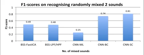
Section III presents various approaches for multi-sound classification. As we are dealing with multiple simultaneous sounds, we use a common metric – F1-score to equally balance precision and recall [1], [14]. To understand their performance on separating sound categories and choose the best approach, we run a small scale experiment. We generate a collection of mixed audio files. Mixing is conducted by randomly selecting two audio files in different sound categories, syncing their duration and then overlaying their signals. In the end, we generate 4.4 hours of mixture audio data from the sound effect dataset. We run each of the approaches on this dataset and calculate their F1-scores, presented in Figure 4.

To configure the BSS-based approach, we attempt two tech-niques: LPF/HPF (high/low pass filter) and ICA. LPF/HPF

can be effective for separating sounds that dominate different frequency bands. For example, a simultaneous mixture of a dishwasher and a milk steamer would result in only the dishwasher being left from using the LPF, and only milk steamer from using the HPF. By first transforming the data into the frequency domain with Fast Fourier Transform (FFT), we then set any desired frequencies to zero (i.e. all low frequencies for HPF, and vice versa), and then return the signal to the time domain by performing an inverse FFT.

We adopt FastICA [6] – another most common and preferred form of BSS. From a multi-channel signal, it can use two

0.49 0.48

0.25

0.74 0.81

0 0.2 0.4 0.6 0.8 1

BSS-FastICA BSS-LPF/HPF CNN-ML CNN-BC CNN-SC

F1

-s

co

re

No. of mixed sounds

F1-scores on recognising randomly mixed 2 sounds

Fig. 4. F1-scores of multi-sound classification on the randomly mixed dataset. BSS-FastICA– BSS approach configured with FastICA in Section III-D.1, BSS-LPF/HPF– BSS approach configured with low/high pass filter in Section III-D.1,CNN-ML– Multi-label classifier after CNN in Section III-D.2, CNN-BC– Binary classifiers after CNN in Section III-D.3, andCNN-SC– a stacked classifier in Section III-D.4.

different mixes of the same multi-class event to distinguish between the sources. When performing ICA, we assume that the sources are statistically independent. To enforce that, we will need to first centre and whiten the data; that is, performing linear transformation to make the components uncorrelated and their variances equal unity.

In BSS-based approaches, we apply bothLPF/HPFandICA

during the pre-processing stage. The resulted separations are then classified using the base CNN, where we add one fully connected layer of 20 neurons (responding to the number of sound categories of interest) after the VGGish network for single sound classification.

For the multi-label sound classifier introduced in Sec-tion III-2, namedCNN-ML, we add one fully connected layer of 210 neurons (responding to the number of sound categories and their combinations). The basic binary classifier approach in Section III-3, named CNN-BC, and the stacked classifier approach in Section III-4, named CNN-SC, will follow the same architecture.

The comparison results are reported in Figure 4. The BSS approaches achieve nearly 50% in classifying a 2-sound mixture. When we look closer at the classification results, it turns out that BSS is better at classifying the dominant sound out of the mixed signal. For example, in the mixture of ‘milk steamer’ and ‘footsteps’, the BSS approaches can always recognise ‘milk steamer’, as it has much higher sound intensity and therefore dominates in the mixed signal. The BSS-based approaches, especially configured with ICA, has worked worse than expected, as when we tested it on a small number of samples, it worked quite well at separating sound classes. By examining the results, we find that the dropped accuracies of ICA in this randomised mixture experiment is due to the fact that the channels for the ICA mixes are too similar to each other, which makes them inseparable. The most effective way of using ICA is to have recordings of simultaneous sounds from two different locations. In this way, there exists one dominant sound in one recording. However, in our model, all the audio data are transformed to contain only one channel, so ICA is not effective in distinguishing similar sounds.

CNN-MLperforms worst, due to a large class set to learn.

of these 210 classes, they are not independent of each other. There exists significant overlapping between different combi-nations that share the same single sound. Such overlapping causes a lot of uncertainty in classification. To understand this

TABLE I

F1-SCORES OFMULTI-SOUNDCLASSIFICATION OFCNN-MLON A

SMALLERCLASSSET

Sound Class F1-score

23 Classes (20 single sound classes + 3 mixes between similar sounds in ‘keyboard’, ‘footstep’, and ‘photo-copier’)

71%

23 Classes (20 single sound classes + 3 mixes between distinct sounds in ‘milk steamer’, ‘phone ringing’, and ‘clear throat’)

89%

26 Classes (20 single sound classes + 6 mixes between the above similar and distinct sounds)

84%

problem deeper, we run another set of experiments on CNN-ML, where we reduce the number of combination classes. That is, we systematically choose three similar and distinct sound categories respectively based on their sound profiles, and mix within and between them, which leads to the results in Table I. CNN-ML can well classify distinct sounds in a mixed signal, with 60% on ‘milk steamer’ and ‘phone ringing’, 84% on ‘milk steamer’ and ‘clear throat’, and 90% on ‘phone ringing’ and ‘clear throat’. By closely examining the results, on the lowest performance 60%, 1% of the time it only recognises ‘phone ringing’ and the remaining 39% of the time it only recognises ‘milk steamer’. Again this is due to the fact that milk steamer has a dominating sound. On the similar mixture, CNN-ML fails to recognise ‘keyboard + footsteps’ and ‘keyboard + photocopier’. For the former case, it only recognises keyboard, while it confuses with photocopier alone and any other mixture with photocopier.

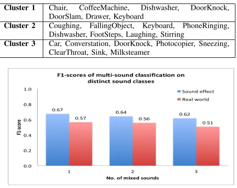
TABLE II

CLUSTERINGSOUNDCATEGORIES

Cluster 1 Chair, CoffeeMachine, Dishwasher, DoorKnock, DoorSlam, Drawer, Keyboard

Cluster 2 Coughing, FallingObject, Keyboard, PhoneRinging, Dishwasher, FootSteps, Laughing, Stirring

Cluster 3 Car, Converstation, DoorKnock, Photocopier, Sneezing, ClearThroat, Sink, Milksteamer

Fig. 5. F1-scores of distinct multi-sound classification.

D. Similarity-driven Mixture

Now we will focus on the final approach CNN-SC to see if it can accurately classify any number of sounds in a mixed

acoustic signal. In order to see if the similarity between sound class has an impact on the performance of the proposed approach, we will systematically mix the sound. We first cluster audio data based on their distances as shown in Table II;

i.e., calculating the Euclidean distance between their extracted MFCC features.

Fig. 6. Accuracies of multi-sound classification on the mixed datasets of similar sound profiles.

Then we can test similar and distinct mixes. To do this, we create new polyphonic files using random selections from each of the clusters, and then only from different clusters. For each number of sound mixture, we generate 1.1 hour audio data of sound effect and real-world data respectively. For the similar mixture, we generate 5.5-hour audio data covering any number of mixture from 1 sound up to 5 sounds. For the distinct mixture, we generate 3.3-hour audio data covering 1-, 2-1-, and 3-sound mixtures1-, equal to the number of clusters. Figure 5 and Figure 6 reports the F1-scores ofCNN-SC, which are categorised on each number of mixture.

with even more complex mixes. Also there is small difference between the test sets, and the real-world recordings are roughly 10% lower on average. This is due to irregularities that come with recordings of real life situations; that is, the strong background noise and high variation in the audio intensity (due to movement in the location of the sound source).

In Figures 6, the rate of degradation does not drastically change when continuing from 3 all the way to 5 mixed events. This indicates that the proposed approach is very robust in dealing with simultaneous activities, even to a high order. It can also be seen that some of the clusters are still classified rather accurately (with the exception of cluster 3), even though they are mixes of similar sound classes. This means that our model remains competent even with ‘hard-to-separate’ mixtures, by finding the unique patterns of the singular events that contribute to the polyphonic sounds.

The results also suggest that the majority of F1-scores decreases when the number of mixed activities increases (with few exceptions, simply caused by the randomly selected files sometimes being easier to distinguish than others). It becomes harder to identify all of the sources, when individual events overlap each other. However, the decrease in performance is not significant, only dropping an average of 6.75% from single to mixed 5 sounds. Our approach, with the use of sound effect data for training only, has achieved comparable accuracies with one recent work [16] that has achieved 65.5% F1-scores when recognising mixed sound from only 10 sound classes by training a RNN on the real-world dataset.

V. CONCLUSION ANDFUTUREWORK

In this paper we explore different approaches for multi-sound classification and propose a novel stacked architecture that outperforms the other alternatives. The evaluation results are promising in that the model performance never drops by a significant amount when going from 1 to 5 mixed events of similar and distinct sound categories. The robustness in multi-sound classification can have a significant implication in many pervasive sensing applications, given that the wide popularity of audio sensing in mobile devices.

The main limitation of our current work is that we have not evaluated on a large-scale real-world audio dataset, which will be our next step. The current experiment methodology allows us to draw a comprehensive performance profile of the proposed approach, by mixing sounds under different conditions. However, in our experiment, we are aware that the real-world audio recordings present quite different acoustic signatures. Investigating additional features to supplement the MFCC will be an interesting direction to explore. Secondly, we only use synthesised sound effect dataset for training, which is beneficial in reducing the reliance on real-world audio data collection and annotation. However, the performance is limited, again due to the difference between synthesised and real-world data. In the future, we will look into more data augmentation techniques to see how to reduce the difference. Also we will assess how much real-world data are needed in training to improve the classification accuracies.

ACKNOWLEDGEMENT

We gratefully acknowledge the support of NVIDIA Corpo-ration with the donation of the Quadro P6000 GPU used for this research.

REFERENCES

[1] E. Cakir, T. Heittola, H. Huttunen, and T. Virtanen. Polyphonic sound event detection using multi label deep neural networks. InIJCNN ’15, pages 1–7, July 2015.

[2] J. Dennis, H. Tran, and E. Chng. Overlapping sound event recognition using local spectrogram features and the generalised hough transform. Pattern Recognition Letters, 34(9):1085 – 1093, 2013.

[3] D. L. Donoho and I. M. Johnstone. Adapting to unknown smoothness via wavelet shrinkage. Journal of the American Statistical Association, 90(432):1200–1224, 1995.

[4] J. F. G. et al. Audio set: An ontology and human-labeled dataset for audio events. InICASSP ’17, New Orleans, LA, 2017.

[5] FreeSound. Found at: https://freesound.org/, Accessed: May 2018. [6] C. Ghita, R. D. Raicu, and B. Pantelimon. Implementation of the fastica

algorithm in sound source separation. InATEE ’15, pages 19–22, May 2015.

[7] T. Hayashi, S. Watanabe, T. Toda, T. Hori, J. Le Roux, and K. Takeda. Duration-controlled lstm for polyphonic sound event detec-tion. IEEE/ACM Trans. Audio, Speech and Lang. Proc., 25(11):2059– 2070, Nov. 2017.

[8] T. Heittola, A. Klapuri, and T. Virtanen. Musical instrument recognition in polyphonic audio using source-filter model for sound separation. In ISMIR, 2009.

[9] S. Hershey, S. Chaudhuri, D. P. Ellis, J. F. Gemmeke, A. Jansen, R. C. Moore, M. Plakal, D. Platt, R. A. Saurous, B. Seybold, et al. Cnn architectures for large-scale audio classification. InICASSP ’17, pages 131–135. IEEE, 2017.

[10] P. Jincahitra. Polyphonic instrument identification using independent subspace analysis. InICME ’04, 2004.

[11] N. D. Lane, P. Georgiev, and L. Qendro. Deepear: Robust smartphone audio sensing in unconstrained acoustic environments using deep learn-ing. InUbiComp ’15, pages 283–294, 2015.

[12] G. Laput, K. Ahuja, M. Goel, and C. Harrison. Ubicoustics: Plug-and-play acoustic activity recognition. InUIST 2018, 2018.

[13] Y. e. a. Lee. Sociophone: Everyday face-to-face interaction monitoring platform using multi-phone sensor fusion. InMobiSys ’13, pages 499– 500, 2013.

[14] A. Mesaros, T. Heittola, and T. Virtanen. Metrics for polyphonic sound event detection. Applied Sciences, 6, 2016.

[15] G. P. Nason. Choice of the Threshold Parameter in Wavelet Function Estimation, pages 261–280. Springer New York, New York, NY, 1995. [16] G. Parascandolo, H. Huttunen, and T. Virtanen. Recurrent neural networks for polyphonic sound event detection in real life recordings. InICASSP ’16, 2016.

[17] J. Park, J. Shin, and K. Lee. Separation of instrument sounds using non-negative matrix factorization with spectral envelope constraints. arXiv:1801.04081, 2018.

[18] T. Park, J. Turner, M. Musick, J. Lee, C. Jacoby, C. Mydlarz, and J. Salamon. Sensing urban soundscapes.CEUR Workshop Proceedings, 1133:375–382, 2014.

[19] J. Portelo, M. Bugalho, I. Trancoso, J. Neto, A. Abad, and A. Serralheiro. Non-speech audio event detection. InICASSP ’09, pages 1973–1976. IEEE, 2009.

[20] K. K. Rachuri, M. Musolesi, C. Mascolo, P. J. Rentfrow, C. Longworth, and A. Aucinas. Emotionsense: A mobile phones based adaptive platform for experimental social psychology research. InUbiComp ’10, pages 281–290, New York, NY, USA, 2010. ACM.

[21] J. Salamon and J. P. Bello. Deep convolutional neural networks and data augmentation for environmental sound classification. IEEE Signal Processing Letters, 24(3):279–283, 2017.

[22] K. Simonyan and A. Zisserman. Very deep convolutional networks for large-scale image recognition.arXiv preprint arXiv:1409.1556, 2014. [23] H. D. Tran and H. Li. Jump function kolmogorov for overlapping audio