Accelerometer-based Orientation Sensing for Head Tracking
in AR & Robotics
Matthew S. Keir
1,2, Chris E. Hann
1, J. Geoffrey Chase
1, and XiaoQi Chen
1 1Department of Mechanical Engineering,
2
Human Interface Technology Lab NZ,
University of Canterbury, Christchurch, New Zealand
[email protected]
Abstract
This work seeks to improve dynamic accuracy of viewpoint tracking for Augmented Reality. Using an inverted pendulum to model the head, dynamic orientation sensing for a single degree of rotation in a vertical plane is achieved using only a dual axis accelerometer. A unique solution is presented as conventional approaches to solve the model equations fail to produce stable results due to ill conditioning. Accuracy is limited by the noise and model error. However, dynamic tracking with better than 1◦accuracy is achieved analytically and experimentally, proving the concept.
Keywords:head tracking, head motion model, inverted pendulum, orientation sensing, accelerometers
1
Introduction
Augmented Reality (AR) systems using head mounted displays (HMDs) require position and orientation (pose) information of the users viewpoint to overlay computer
imagery correctly. Tracking accuracy and system
latency are crucial to providing a compelling and useful AR application. Robust tracking systems are available for quasi-static applications. However, when applied in more dynamic applications they fail to produce the accuracy required.
Many different technologies have been applied to the head tracking problem, although no one technology tracks well for all applications [1]. As a result hybrid approaches have been taken ([2], [3], [4]) to improve accuracy and robustness by utilising two or more complementary technologies. Inertial tracking is often included in such approaches.
The inertial measurement units (IMUs) used for head tracking usually contain micro-electro-mechanical systems (MEMS). Specifically, rate gyroscopes (gyros)
and accelerometers. High update rates and small
size reduces system latency and allows unobtrusive
packaging. However, measurements from these
accelerometers and gyros require integration to obtain position and orientation. Numerical integration of noisy signals causes the results to drift. For the gyro this drift requires correction. However with the accelerometer drift corrupts the position measurement entirely due to the double integration required. Hence, inertial devices are only useful for tracking orientation in this application. Importantly AR systems are more sensitive to orientation error than position error, as the orientation error is scaled by the distance to the viewed object [5].
Accelerometers sense dynamic accelerations and also
the acceleration due to gravity. As a result
accelerometers can be very useful in tilt or orientation applications. For a stationary object determining
the orientation with respect to gravity is a trivial problem. However, when other motion is introduced the acceleration signal is modified by the dynamic accelerations, leading to orientation errors.
One approach to this problem is to take advantage of the burst like nature of head motion and correct for gyro drift during natural pauses [6]. However [7], shows orientation is improved using accelerometers to aid the gyroscope during human kinematic measurement, but does not detail the motion. Thus a full solution using only one sensor is lacking.
Commercial IMUs suitable for tracking 3DOF head motion include, the InertiaCube3 [8], 3d-Bird [9],
MTx [10] and the 3DM-DH [11]. These IMUs
typically contain three rate gyros, accelerometers and
magnetometers. However, these devices are not
optimised for individual applications although some allow the user to define initial filtering. None are yet fully proven in a highly dynamic environment.
Head motion for most applications is well below 2 Hz [12]. However, applications such as outdoor gaming
demand much higher dynamic performance. Most
approaches to improving dynamic tracking involve using Kalman filtering to fuse data from different sources and provide prediction to reduce system latency [13], [14]. The Kalman filter uses a model of the motion to predict for the next iteration step, this is not feasible with an unstable or unknown head motion model.
This paper seeks to improve inertial sensing for pitch and roll in a highly dynamic environment using
minimal numbers of low cost sensors. Using an
2
METHOD
2.1
Model – Rotation in a Vertical Plane
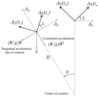
[image:2.595.70.278.310.515.2]An inverted pendulum is used to model the head with a dual axis accelerometer positioned along the pendulum, in the plane of rotation. The radius of rotation for the head may be a function of the degree of rotation. However, for this proof of concept the radius is considered to be fixed.
Figure 1 shows the components of acceleration applied to a particle at radius R for in-plane rotation (θ) of the head or pendulum. These tangential, centripetal and gravitational (g) accelerations and are sensed by the accelerometer axes Ay and Ax. The accelerometer is positioned at a fixed angleλ to the tangent of rotation, whereλ =π/4 provides optimal sensitivity to gravity on both accelerometer axes. It also ensures the other accelerations are sensed by both axes which is useful to abate noise.
Ax(t )0
Ax(t )1
AT AT
AR
R
g
q l
l Ay(t )1
Ay(t )0
(R/g)θ¨
Tangential acceleration due to rotation
(R/g)θ˙2 Centripetal acceleration
[image:2.595.317.514.502.640.2]Centre of rotation
Figure 1: Acceleration vector diagram for a point at the end of an inverted pendulum, length R, undergoing
a rotation ofθ
The tangential (AT(t)) and radial (AR(t)) accelerations are derived from the measured accelerations below. Note that all accelerations and rotations (θ(t)) are functions of time and that the “(t)” is dropped for clarity.
AT =Axcos(λ)−Aysin(λ), (1)
AR=Axsin(λ) +Aycos(λ). (2)
The accelerometer senses the acceleration of its proof mass relative to its casing. Hence, dynamic accelerations contribute in the opposite direction to that shown in figure 1. Resolving acceleration in terms of g along the tangential and radial axes provides two
independent ordinary differential equations (ODEs) for
AT and AR:
AT= (R/g)θ¨−sin(θ), (3)
AR= (R/g)θ˙2−cos(θ). (4) It is important to note that these are not equations of motion, and are thus is independent from any inertia, actuation force, damping or physiological limits that may influence the motion. The effect of any such terms will directly contribute the measured acceleration and is therefore captured by this model. This approach frees the problem from complex calibration or system identification procedures.
2.2
A General Engineering Approach
Solving equations (3) or (4), should provide the solution forθ. As a first attempt, data is generated forθ from a modified sine wave. The tangential acceleration is determined by substituting θ into equation (3). This ODE was solved in Maple using the default initial value problem (IVP) solver, a Fehlberg fourth-fifth order Runge-Kutta method, and in Matlab using a similar solver. Both Maple and Matlab failed to produce a stable solution.
Providing the solver with the actual initial conditions, θ(0)and ˙θ(0), results in the solution tracking the true solution for only two cycles before diverging. This result represents the pendulum spinning in the real system. Figure 2 shows that with a very low amplitude forθ the solution almost stabilises atπ. Similar quasi-stability can be found at−π when the pendulum is no longer inverted, a stable solution for the real pendulum. Including a damping term in the ODE can stabilise this solution. However, it proves to be of no use in determining the true rotation.
True Solution Solved Solution 0
2 4 6 8 10
theta (rad)
2 4 6 8 10 12 14
time (s)
Figure 2: Simulated data, solved numerically. Note the that the solved solution oscillates around Pi before
blowing up completely
A second attempt combines the Equations, (3) and (4). Solving simultaneously also fails to produce a stable result. To gain a better understanding of the instability of the model and enable an analytical solution Equation (3) is linearised:
Giving an analytic solution of the form:
θ=C2e
√ g √
Rt+C
1e
− √
g √
Rt−A
T (6)
where C1and C2are constants. The positive power on the C2exponential term leads to instability. The system is extremely sensitive the the value of the C2 and thus the initial conditions.
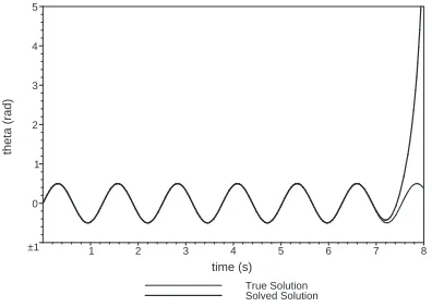
To illustrate this issue consider synthetic data generated from equation (5). Solving using the exact initial
conditions provides the true solution. However,
introducing a small error to the ˙θ initial condition ε makes the solution unstable. Figure 3 illustrates this ill conditioning when the error is ε =1e−18. Even recursive approaches over a much shorter period will not work because any error will quickly grow and corrupt the solution.
True Solution Solved Solution –1
0 1 2 3 4 5
theta (rad)
1 2 3 4 5 6 7 8
[image:3.595.80.278.273.414.2]time (s)
Figure 3: Simulated linearised data, solved analytically using initial conditions with a small error
2.3
Feasible Solution Method
It is clear that this challenging problem requires a
novel approach. This section presents a unique
solution independent from initial conditions to obtain
C2with the precision required to give accurate rotational measurement.
Equation (3) is solved over a short period of time. Fitting a cubic function to AT and ARover this period effectively filters higher frequency noise:
AT,f it=u1+u2t+u3t2+u4t3 (7)
AR,f it=v1+v2t+v3t2+v4t3 (8)
Substituting equation (7) into equation (3) and making a linear substitution for sin(θ)gives:
AT,f it= (R/g)θ¨−(b1+b2θ) (9) where b1and b2are evaluated by a linear least squares fit to for the past values of θ. A piecewise function improves the fit and allows a longer period to be solved over. However, a separate ODE must be generated and solved for each interval.
Solving equation (9) gives θsol, the solution for the tangential ODE, defined analytically as:
θsol=C2e(mt)+C1e(−mt)+f(t) (10)
where C1and C2are unknown constants and:
m=
p (b2g)
√ R
f(t) = 1
b22g
µ
−gb2(b1+a1+a2t+a3t2+a4t3)
−2R(3a4t+a3) 
If a piecewise substitution for sin(θ)is used in equation (9) then all except the first ODE will have initial conditions defined by the previous equation in terms of C1and C2. Analytical solutions to these subsequent ODEs can be formed, though take up to much space to be shown here. Solving the set of ODEs generates a piecewise solution forθsol.
Equation (10) is very sensitive to the value of C2, as illustrated earlier. The approach taken here is to utilise the independent radial equation (4), to solve for C1 and C2. Substituting θsol into this equation and approximating cos(θ) by a least squares fit to a quadratic function over the whole period gives:
AR,sol= (R/g)θ˙sol2−(c1+c2θsol+c3θsol2) (11)
To find the optimal C1 and C2 values a least squares approach fits AR,sol to the radial acceleration, equation (8), over the period. Two independent equations are required which are obtained by differentiating with respect to each constant.
EqA=
d dC1
µ p
∑
i=1
³
AR,sol(t−i)−AR,f it(t−i) ´2
(12)
EqB=
d dC2
µ p
∑
i=1
³
AR,sol(t−i)−AR,f it(t−i) ´2
(13)
where p is the number of data points in the period solved over.
Simultaneously solving equations (12) and (13), provides nine pairs of solutions. The real pair that minimises the following equation are selected.
EqC=
µ p
∑
i=1
³
AR,sol(t−i)−AR,f it(t−i) ´2¶1/2
(14)
The selected C1and C2are substituted into equation (10) to give orientation for the current time step. The vector containing the past orientation,θoldcan then be updated ensuring an accurate fit is achieved for the trigonometric substitutions in equations (9) and (11) for the next time step. Figure 4 summarises this method in a flow-chart.
2.4
Analysis and Performance Metrics
• Verify the model using experimental data from an inverted pendulum.
• An analysis to determine the robustness to noise using synthetic data.
• Determine the dynamic performance of the
method.
• Test the method with experimental data.
To measure and quantify performance, the mean absolute error and percentage this is of the mean
amplitude of the signal are calculated. For the
synthetic data, error is defined as the difference
between the solution and θ used to generate the
acceleration signals. For the experimental data the error is the difference between the solution and the optical encoder measurement. Standard deviation and maximum error will measure the spread of the fit. These performance metrics are calculated after any initial transient behaviour in the solution has died away.
Approximate cos(theta) Ax measured
Ay measured
A Tangential Acceleration, Eq. (1)
T
Filter: Least Squares cubic fit AT, f it, Eq. (7)
Solve the ODE(s), Eq. (9), to give Eq. (10)
Generate A in terms of C and C , Eq. (11)
R, sol 1 2
Solve for C and C using Least Squares fit A to A
Eq. (12) and Eq. (13)
1 2 R, sol R, f it
Select the minimum LS solution, Eq.(14)
Substitute C and C into Theta , Eq. (10), and evaluate for the next time point
1 2 sol
Theta Solution
[image:4.595.75.277.320.727.2]Approximate sin(theta) Theta old
Figure 4: Flow-chart for the solution ofθ
3
RESULTS AND DISCUSSION
3.1
Model Verification
To verify that equations (3) and (4) fit the model of the inverted pendulum a simple experiment was conducted. An existing inverted pendulum apparatus was used with an optical encoder providing an independent measure of rotation,θen. An Analogue Devices ADXL213 dual axis accelerometer was attached to the pendulum at radius R=0.3m, and at an angleλ =43.4◦. Data was collected while manually oscillating the pendulum at a slow frequency.
Estimates of the true AR and AT were generated
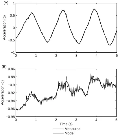
using θen and the model equations (3) and (4). To combat the buildup of noise due to the differentiation of θen, this signal was filtered to smooth the steps caused by the finite resolution of the encoder. The measured accelerations Axand Ay were resolved along the tangential and radial axes using equations (1) and (2). A comparison of the model acceleration with the measured accelerations is shown in figure 5.
0 1 2 3 4 5
−1 −0.5 0 0.5 1
Acceleration (g)
(A)
0 1 2 3 4 5
−0.98 −0.96 −0.94 −0.92 −0.9 −0.88 −0.86
Acceleration (g)
Time (s) (B)
[image:4.595.315.519.326.559.2]Measured Model
Figure 5: Measured and model tangential (A) and radial (B) acceleration
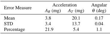
The mean, standard deviation (STD) and percentage errors are summarised in table 1. A percentage error of 5.4% relative to the mean amplitude shows a good fit between the measured tangential acceleration and the model. However, 21.9% shows the error is much worse for the radial acceleration due to poor sensitivity to orientation when this axis is near vertical.
To determine the accuracy of the model fit to the experimental data in terms of θ, independently from the solution method and noise, equation (3) is integrated giving:
θ=g
R Z t
0
Z t
0
AT+
g R
Z t
0
Z t
0
sin(θ) +t ˙θ(0) +θ(0), (15)
determines the optimal initial conditions ˙θ(0) and θ(0). This method could also be used to find an optimal R value for later calibration procedures, but here the measured R is used. Evaluating the fit allows an estimate of the model error in terms of theta to be calculated.
The model error is evaluated for each subsequent 0.3s second period. This is the same period that algorithm presented is solved over for each iteration. The final column in table 1 shows the maximum mean error for any section. This error is much less than 1◦ or 1.1% of the mean signal amplitude in a highly dynamic situation and verifies that the inverted pendulum model does capture the main dynamics for this situation. Explanations for the remaining model error include:
• Missing dynamics due to finite encoder precision.
• Errors in the initial set up, placement of the accelerometer, and zero position of the pendulum.
• Out of plane disturbances affecting the
[image:5.595.314.519.70.308.2]accelerometers.
Table 1: Angular and acceleration model error
Error Measure Acceleration Angular
AR(mg) AT(mg) θ(deg)
Mean 3.8 20.1 0.17
STD 3.4 13.7 0.04
Percentage 21.9 5.4 1.1
3.2
Robustness to Noise
Noise on the acceleration signals which drive the solutions to the ODE are comprised of two sources.
First, the high frequency raw noise from the
accelerometer and circuitry. Second, a lower frequency model error that may include motion not captured by the encoder. The method developed is tested using synthetic data at three noise levels and two different linearisation approaches for sin(θ)in equation (9).
The noise applied to the synthetic acceleration signals was derived from the mean percentage error in table 1. A single interval of 0.1s was used in the linearisation in Method (A) and a three section piecewise function over 0.3s in Method (B). Results are shown in table 2 and figure 6. A static calculation of rotation is included in the figure for comparison. This simple approach assumes that the change in tangential acceleration is due only to the gravitational component. Thus, taking the inverse sine of AT yieldsθsimple.
Table 2: Error response to the presence of noise
Noise Max (deg) STD (deg) Mean (deg) %
(A) None 0.14 0.01 0.001 0.02
Mean 2.0 0.39 0.42 6.8
2×Mean 2.9 0.56 0.63 10.0
(B) None 0.17 0.02 0.005 0.08
Mean 1.1 0.19 0.17 2.8
2×Mean 1.6 0.28 0.30 4.7
0 0.5 1 1.5 2 2.5 3 3.5 4 −0.2
−0.1 0 0.1 0.2 0.3 0.4
Theta (rad)
(A)
0 0.5 1 1.5 2 2.5 3 3.5 4 −0.2
−0.1 0 0.1 0.2 0.3 0.4
Theta (rad)
Time (s) (B)
[image:5.595.86.270.348.405.2]True Solution Solved Solution Simple Solution
Figure 6: Results for simulated data with mean noise applied solved using Method (A) and Method (B)
Both methods produce results where the mean error is less than 1◦. However, Method (B) shows superior performance with approximately half the error and reduced spread in results. For the case where mean noise is applied the maximum error is just over 1◦. Solving over a longer period captures more dynamics increasing the amount of signal relative to the noise present. This improves the nine solutions for C1 and
C2and reduces the uncertainty in selecting the correct pair in equation (14).
Further improvements can be achieved by optimising the accelerometer placement. Aligning ARwith gravity gives poor sensitivity to static rotations along this axis. This is illustrated in figure 5 with the measured AR having a very small amplitude and a huge mean error of 21.9%. The radial equation is not solved, it is used to determine the constants C1and C2in the solution of the tangential equation using a least squares fit. Though, this method is robust in terms of the noise on AR, improving the signal amplitude increases the accuracy in the final result. Although not practical for all situations, this is achieved by shifting the accelerometer so that it is not directly above the centre of rotation. Hence, separating the vertical and radial axis.
3.3
Experimental Results
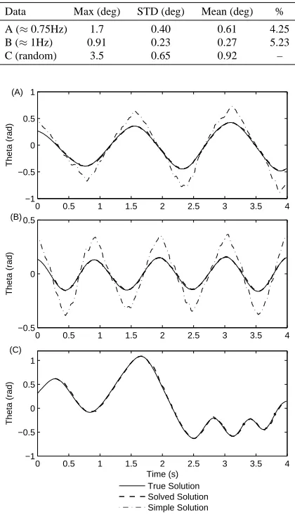
[image:5.595.71.286.683.762.2]Table 3: Experimental error results
Data Max (deg) STD (deg) Mean (deg) %
A (≈0.75Hz) 1.7 0.40 0.61 4.25
B (≈1Hz) 0.91 0.23 0.27 5.23
C (random) 3.5 0.65 0.92 –
0 0.5 1 1.5 2 2.5 3 3.5 4 −1
−0.5 0 0.5 1
Theta (rad)
(A)
0 0.5 1 1.5 2 2.5 3 3.5 4 −0.5
0 0.5
Theta (rad)
(B)
0 0.5 1 1.5 2 2.5 3 3.5 4 −1
−0.5 0 0.5 1
Theta (rad)
Time (s) (C)
True Solution Solved Solution Simple Solution
Figure 7: Experimental results for (A), (B), and (C) data sets compared toθen
4
CONCLUSIONS
Viewpoint tracking methods for augmented reality applications that use HMDs generally suffer from poor
dynamic performance. This work achieves dynamic
orientation tracking for a single degree of rotation in the vertical plane using only a dual axis accelerometer. Head motion is modelled by that of an inverted pendulum, however instability in the model results in ill conditioning and can not be solved using conventional
methods. A unique approach that is independent
of initial conditions is presented and evaluated with synthetic and experimental data.
The algorithm presented produces good results with mean error better than 1◦for synthetic and experimental data. The integrity of this result is maintained as the dynamics are increased and it does not suffer from drift. The accuracy of the solution is limited by the model error and noise. Latency introduced by this solving method has not been considered. This work proves the initial concept of using an accelerometer to measure dynamic head rotation in a vertical plane.
5
References
[1] G. Welch and E. Foxlin, “Motion Tracking: No Silver Bullet, but a Respectable Arsenal”, IEEE
Computer Graphics and Applications, 22(6), pp
24–38 (2002).
[2] G. W. Roberts, A. Evans, A. Dodson, B. Denby,
S. Cooper and R. Hollands, “The use of
augmented reality, GPS, and INS for subsurface data visualization.”, in FIG XXII International
Congress, Washington, D.C (2002).
[3] S. You, U. Neumann and R. Azuma, “Orientation
Tracking for Outdoor Augmented Reality
Registration”, IEEE Computer Graphics and
Applications, 19(6), pp 36–42 (1999).
[4] E. Foxlin and L. Naimark, “VIS-Tracker: A
Wearable Vision-Inertial Self-Tracker”, in VR, pp 199–206, IEEE Computer Society (2003).
[5] R. L. Holloway, “Registration Error Analysis for
Augmented Reality”, Presence: Teleoperators
and Virtual Environments, 6(4), pp 413–432
(1997).
[6] E. Foxlin, M. Harrington and Y. Altshuler, “Miniature 6-DOF inertial system for tracking HMDs”, in Proceedings of the SPIE, volume 3362, pp 214–228, Orlando, FL (1998).
[7] H. Luinge, P. Veltink and C. Baten, “Estimation of orientation with gyroscopes and accelerometers”, in BMES/EMBS Conference, 1999. Proceedings of
the First Joint, volume 2, p. 844 (1999).
[8] Inetersense Inc, “Home Page”,
http://www.isense.com/, visited on 1/8/ 2007.
[9] Ascension Technology Corporation, “Home
Page”, http://www.ascension-tech.com/, visited on 1/8/ 2007.
[10] Xsens Technology, “Home Page”,
http://www.xsens.com/, visited on 1/8/ 2007.
[11] Micro Strain, “Home Page”, http:
//www.microstrain.com/, visited on 1/8/ 2007.
[12] R. Azuma and G. Bishop, “A
frequency-domain analysis of head-motion prediction”, in
SIGGRAPH, pp 401–408 (1995).
[13] E. Kraft, “A Quaternion-based Unscented Kalman Filter for Orientation Tracking”, in Proceedings of
the 6th Int. Conf. on Information Fusion, Cairns,
Australia (2003).
[14] L. Chai, K. Nguyen, B. Hoff and T. Vincent, “An Adaptive Estimator for Registration in Augmented Reality”, in Proceedings of IEEE International
Workshop on Augmented Reality, pp 23–32 (1999).
[15] C. Shaw and J. Liang, “An experiment to characterize head motion in VR and RR using MR”, in Proceedings of the 1992 Western