Towards an Interactive Drone,
A Bayesian Optimization Approach
A. (Asem) Khattab
M
Sc Report
Committee:
Prof.dr.ir. S. Stramigioli
Dr.ir. J.B.C. Engelen
R. Hashem, MSc
Dr. M. Poel
August 2018
030RAM2018
Robotics and Mechatronics
EE-Math-CS
University of Twente
iii
Summary
For a drone, equipped with an impedance controller, to correctly deal with physical contact and interaction with the environment, the impedance parameters should be adjusted correctly depending on the interaction task.
Concentrating on interaction tasks requiring a constant set of impedance parameters values throughout operation. A model-free learning framework is proposed to automatically find the suitable parameters values. The framework relies on Bayesian optimization and episodic re-ward calculation requiring the drone to repeatedly perform a predetermined task in the envi-ronment actively searching in the impedance parameters space.
The sample-efficiency and safety of learning were improved by adding two novel modifications to Bayesian optimization. The first one is local optimization of acquisition functions allowing learning to get early warnings during exploration. The second one is conditioning the reward signal with a logistic function exploiting the initial knowledge and enabling generalizing learn-ing settlearn-ings to different situations.
Contents
1 Introduction 1
1.1 Related Works . . . 2
1.2 Problem Formulation and Challenges . . . 2
1.3 Proposed Method . . . 5
1.4 Research Questions . . . 6
1.5 Report Layout . . . 6
2 Bayesian Optimization Framework 7 2.1 Background . . . 7
2.2 Surrogate Model . . . 10
2.3 Initial Knowledge . . . 11
2.4 Acquisition Functions . . . 13
2.5 Conclusion . . . 15
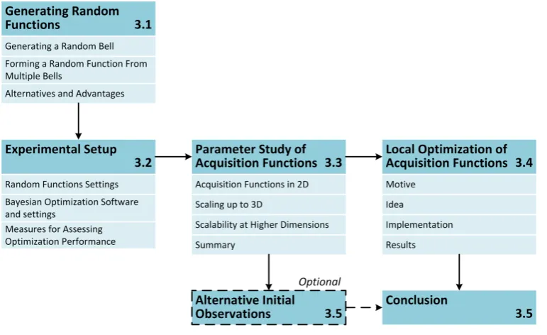
3 Bayesian Optimization Empirical Studies 17 3.1 Generating Random Functions . . . 18
3.2 Experimental Setup . . . 21
3.3 Parameter Study of Acquisition Functions . . . 23
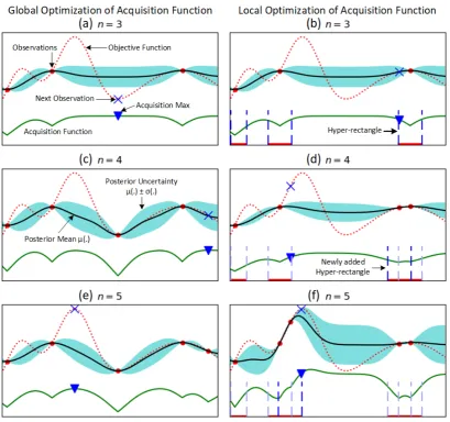
3.4 Local Optimization of Acquisition Functions . . . 32
3.5 Alternative Initial Observations . . . 38
3.6 Conclusion . . . 41
4 Simulation Results and Discussion 42 4.1 Simulation Description . . . 42
4.2 Reward Shaping . . . 45
4.3 Experimental Setup . . . 50
4.4 Results and Discussion . . . 54
4.5 Conclusion . . . 64
5 Reinforcement Learning Point of View 65 5.1 Background . . . 65
5.2 Problem Formulation as a Continuum Bandit . . . 67
5.3 Bayesian Optimization and Reinforcement Learning . . . 68
Conclusion and Future Work 70
A Impedance Control 73
B Simulation Software Implementation Details 74
1
1 Introduction
With their high mobility, drones can be employed in various industrial tasks significantly de-creasing their cost. Examples include inspection of high structures like wind turbines, cell tow-ers and power lines. There is a mature research body in position control of drones with com-mercial products already available in the market. Drones are now well capable of handling all tasks requiring mere free flight. Exploiting advances in other fields like machine learning, com-puter vision and path planning, drones can perform a wide range of tasks like object identifying and tracking as well as surveying and imaging.
However, there is still much research work to be done to allow drones to handle interaction and contact tasks with the environment. In these situations, the force applied by the drone on the environment is of great influence to the success of the task. Motion control alone turns out to be unsuitable as the unavoidable modeling errors and uncertainties can cause the contact force to rise, leading to an unstable behavior during the interaction, especially in the presence of rigid environments [31]. To solve this issue, several control schemes have been proposed in the literature known as interaction (or force) control schemes. While these schemes have been extensively studied and experimentally applied for robotic manipulators, there is a lack in literature in their application to drones.
Interaction control is an essential requirement for a successful employment of drones in in-dustrial applications as it will give them the ability to perform direct contact tasks like parts insertion and replacement as well as surface polishing and writing. With these capabilities, a drone can be easily used to handle, for instance, the maintenance of wind turbines.
One of the most widely used interaction control schemes is impedance control [31]. The robot (the drone in our case) then behaves as an impedance in the environment modeled as a mass-spring-damper system with adjustable parameters. Adjusting these controller’s parameters properly, one can achieve a compliant behavior (where the robot is more lenient with the dis-turbances imposed by the environment) or a stiff behavior (where the robot is more precise in tracking a goal and more stable against unpredictable disturbances). The main problem is: selecting good impedance parameters ensuring the desired behavior is not an easy straightfor-ward task [31]. It requires either an accurate model of the environment where the contact will occur or a human expert tuning the parameters simply by trial and error. The parameters val-ues that will result in a satisfactory performance heavily depend on the nature of the task and the physical and dynamic characteristics of the drone and the environment.
It was noted that it is the ability to quickly adapt the impedance parameter of the body to the faced situation that allows human and other biological systems to have a robust and safe in-teraction with the environment [28]. In fact, some sports are harder to master because they require more precise balance between compliance and stiffness. It can take humans more than two decades to develop and tune this balance [28]. Giving this learning ability to robots is the key towards robust and safe robotic interaction.
1.1 Related Works
In general, active interaction control schemes can be divided to two main categories: direct and indirect force control. In direct force control, the contact force and moment are explicitly controlled with a force feedback loop. This requires reasonably precise 6D force measurements. Instead, in this thesis, we work with indirect force control. One of the well known and widely used schemes in this category is impedance control, where the deviation of the end-effector motion from the desired motion due to the interaction with the environment is related to the contact force through a mechanical impedance. For more, see Appendix A.
Techniques of learning impedance parameters in literature vary depending on the application and usage of the impedance controller. In a medical application, human demonstrations were employed to learn impedance parameters for a lower-limb prostheses [3]. The scope of the technique is limited to situations where demonstrations of the correct behavior can be easily obtained and the number of needed demonstrations is small.
Learning by demonstration is more connected to supervised learning than it is to reinforce-ment learning. The agent in this case does not perform any form of trial-and-error. It directly infers the parameters values from the demonstration. Hence, it is not suitable for general au-tonomous learning in unpredictable environments and dynamics. Only reinforcement learn-ing can offer a general learnlearn-ing approach that can deal with different unpredictable situations.
Another supervised-learning-based method was proposed in [19], where a model of the dy-namics is learned using locally weighted projection regression. This model is then used to derive an optimal control policy for variable impedance actuators. In addition to lacking the interactive learning feature in reinforcement learning, the accuracy of this method is limited by the level of details in the physical model and the precision of identifying this model through supervised learning.
Other works investigated learning atrajectoryof impedance parameters such that the param-eters values vary with time depending on the need of the task. For example, in [6, 28], theP I2
algorithm (policy improvement with path integrals) is used to learn impedance parameters trajectories (gains schedules) for robots with high degrees-of-freedom. The work combines as-pects form optimal control and reinforcement learning to train robots to do tasks like flipping a light switch and pushing open a door. During such tasks, both the position trajectory and the impedance parameters trajectories are learned.
While such methods have the advantage of being model-free and hence able to deal with dif-ferent environments and unpredictable situations, they suffer from two main problems. The first one is that the learning is very specific to the task. For example, if the size of the switch, its weight or its stiffness changes, the whole switch flipping task needs to berelearned. Further, because the learning objective is to find a trajectory of the parameters along time not a fixed set of parameters, the state-action space is huge, which requires a large number of iterations (tri-als) for the learning to reach reasonable results. To remedy this, kinesthetic teaching (moving the robot by hand to do the task) is used to give meaningful initial trajectories. Still, learning needs more than a hundred updates to converge.
1.2 Problem Formulation and Challenges
Given an interaction controller (impedance/admittance) implemented on a drone, the goal of this thesis is to devise a suitable framework for model-free learning of the optimal controller’s parameters values for achieving a certain interaction task. The focus is on tasks requiring a fixed set of parameters values throughout operation. Examples of such tasks include surface contact tasks like polishing, cleaning and writing.
CHAPTER 1. INTRODUCTION 3
aerodynamics play a significant role. The aim is to perform efficient trial-and-error learning to automatically find the optimal parameters values. The idea is illustrated in Fig. 1.1. The drone, with its initial set of parameters values, performs unsatisfactorily (left circle) in the task of drawing a circle as the physical characteristics of the arbitrary surface are unknown to the user. Through smart trial-and-error, the drone learns impedance parameters values that give better performances (middle circle). By the end of training (or learning), the drone finds the optimal set of parameters values (right circle).
Figure 1.1:A drone training to find optimal impedance parameters for drawing a circle on a surface with unknown physical characteristics.
It can be realized that the task of finding the optimal set of impedance parameters values is actually equivalent to the optimization of an expensive black-box function. The function be-ing optimized f(x) represents a performance measure for the drone under a selected set of impedance parameters valuesx. We call it the reward function. It is black-box because there is not a closed form mathematical expression for the function in terms of the parameters values
x. Otherwise the problem can be solved without learning. Instead, the function is costly eval-uated at a certain pointx(a certain set of impedance parameters values) by observing the per-formance of the drone while doing an application-specific predetermined task (like following a trajectory to draw a circle as in Fig. 1.1). Based on that,f(x) gives a single number indicating how satisfactory the performance was.
The learning problem becomes then the problem of finding the position of the global maxi-mum of that black-box reward functionx∗=arg maxf(x) using as few evaluations as possible to minimize the learning cost. A simple block diagram of the learning problem is shown in Fig. 1.2.
Figure 1.2:Simple block diagram of the proposed learning problem formulation.
The main goals of this work are then to find a suitable technique for autonomously learning the optimal parameters values for a task (by optimizing the black-box reward function), adapt this technique to the problem at hand considering the limitations imposed by working with a robotic drone system, and finally validate the proposed method via simulations.
Challenges
Achievement of these goals is a challenging task. Two challenges should be highlighted for their significant influence. The first one is the high cost of learning. Aside from the power costs of operating the drone, operation cannot be done without human supervision. In addition, in case of crashes due to instability or bad performance often encountered during exploration (trying new impedance parameters values) in learning, fixing the drone is expensive financially and time-wise. For that, to be suitable for the problem, the learning method has to be sample-efficient such that it doesn’t require much operation time to learn.
The second challenge is the continuity and high dimensionality of the parameters space. The number of impedance parameters to learn (the degrees-of-freedom in this learning problem) can reach 27 (See Appendix A for details). It is very challenging to find an interactive learning technique that scales up to this high number of dimensions with few samples (short operation time). Other approaches can be also taken to go around this high dimensionality problem. One of them is reducing the dimensionality of the learning depending on the task by adding constraints on the parameters values.
CHAPTER 1. INTRODUCTION 5
1.3 Proposed Method
In this thesis, an episodic learning framework is proposed. The proposed framework is illus-trated in Fig. 1.3. At each episode, the drone receives a set of parameters values. The impedance is configured according to the received values and then the drone performs a task designed by the user to assess the performance of the chosen impedance settings. In our case, this task is following a prescribed trajectory (sent from the motion planner). While performing the task, all relevant sensory measurements (from on-board sensors or off-board ones in the environment) are stored and can be also used to detect any failure in real time. In case the task was com-pleted successfully, the stored sensors measurements are used to compute the reward (the per-formance measure) which can include different elements (For example, the root-mean-square (RMS) of the position error) depending on the objective of the learning. This reward is sent back to the learning algorithm, which should intelligently select another set of parameters val-ues to try in order to quickly find a satisfactory set of parameters valval-ues (a one that gives a high reward). If a failure is detected, the impedance settings are all restored to safe default values and a very small reward (or a penalty in this case) is returned to the learning algorithm indi-cating that the performance was highly undesirable. This failure reward is application-specific and is given by the user.
Figure 1.3:Simplified block diagram of the proposed learning framework.
As mentioned in section 1.2, the learning block in Fig 1.3 works on finding the position of the global maximum of the black-box reward functionx∗=arg maxf(x) where:
• xis a vector containing the selected impedance parameters values.
• f(x) represents a performance measure of the drone in the interaction task under the selected impedance parameters values.
incor-porating human expert knowledge or intuition, if available, in the learning. Above all of that, it scales polynomially with the number of dimensions escaping the curse of dimensionality (the need for exponentially more data and computations as the number of dimensions grows). To the author’s best knowledge, this thesis represents the first research effort to apply Bayesian optimization for learning impedance parameters.
1.4 Research Questions
The initial question addressed in this thesis was:
RQ1. Which model-free method is suitable for automatically learning a single set of impedance parameters values for a drone interacting in the environment?’.
After surveying the literature in section 1.1 and formulating the problem as in section 1.2, Bayesian optimization was found to be the suitable solution for the reasons mentioned in sec-tion 1.3.
Given the proposed learning framework that uses Bayesian optimization, the following re-search questions arise:
RQ2. How to adapt Bayesian optimization to the requirements and limitations faced in learn-ing impedance parameters values for a drone.
RQ3. How to apply the proposed learning framework to find impedance parameters values for an interaction task and verify its validity in a simulated environment?
The rest of this thesis is dedicated to answering these two questions.
1.5 Report Layout
The rest of this thesis is arranged as follows:
Chapter 2: Explores the different components of the Bayesian optimization framework and discuses its design space making suitable choices with respect to the application at hand.
Chapter 3: Investigates the performance of Bayesian optimization with different settings by applying it to simulated randomly generated black-box functions with different numbers of dimensions. The gained insights from these results are then used to innovate an effective mod-ification to the Bayesian optimization framework making it safer and more efficient.
Chapter 4: Discusses how to design a reward function presenting a novel modification to the Bayesian optimization framework improving its sample-efficiency. After that, the results of ap-plying the proposed framework to a simulated drone for learning impedance parameters values for sliding tasks are displayed and discussed
Chapter 5: Provides another perspective into the proposed learning framework as a reinforce-ment learning method.
7
2 Bayesian Optimization Framework
Bayesian optimization is a framework for sample-efficient search for the extremum (the maxi-mum or the minimaxi-mum) of a black-box function. That is a function that can only be evaluated or inquired (even via noisy observations) at any arbitary point in its domain. Bayesian optimiza-tion is particularly useful for situaoptimiza-tions where the target funcoptimiza-tion has no closed-form expres-sion, is difficult to get derivatives for, is very expensive to evaluate and/or is non-convex [5, 24].
In this chapter, the different elements of the design space of Bayesian optimization are explored making suitable choices with respect to the application of learning drone’s impedance param-eters. The chapter starts with a background about the principles of Bayesian optimization and a brief survey of its notable applications in section 2.1. Section 2.2 discusses the probabilistic surrogate model and describes Gaussian processes. Section 2.3 investigates the different ways Bayesian optimization offers for incorporating initial human knowledge (or intuition) in the learning. Section 2.4 touches on the main acquisition functions found in literature describing the intuition behind them. Finally, the chapter is concluded by summarizing the main assump-tions and decisions made when using Bayesian optimization for the application at hand.
2.1 Background
Formally, the goal of Bayesian optimization is to find the positionx∗of the global maximum (or minimum) of an unknown target functionf(x):
x∗=arg max
x∈χ f(x) (2.1)
whereχis the (multi-dimensional) domain of the target function.
There exists a solid body of research in mathematics for this kind of problems. However, the suggested methods require a large number of evaluations to guarantee reaching the global maximum. Moreover, the number of needed evaluations grows exponentially as the number of dimensions of the problem increases [14, 5]. Such number of evaluations is impractical for expensive-to-evaluate functions, like the one we are considering here.
Instead of relying on the density of evaluations, Bayesian optimization takes a different ap-proach towards the problem. It exploits all the evaluations it can get by building a surrogate model that represents the current belief about the black-box function. It uses this model to de-cide where to prop (evaluate) the function next in order to make the position of the maximum of the surrogate model as close as possible to the position of the maximum of the black-box function. The decision of the next point to prop is carried out viaacquisition functions, which provide a way to balance exploration (trying at positions where there is more uncertainty about the value of the target function) and exploitation (trying at positions where the current belief shows the target function has a high value).
The name ‘Bayesian’ comes from the fact that the framework relies on one of central theorems in statistics known as Bayes’ Rule. The theorem simply states that theposteriorprobability of a model (or hypothesis)Mgiven evidence (or observations)Eis proportional to thelikelihood
ofEgiven M multiplied by thepriorprobability ofM:
P(M|E)∝P(E|M)P(M) (2.2) The used terminology emphasizes the sequential nature of the process of updating our model. We begin by having aprior info about the probability of the modelP(M). After obtaining a certain evidence (or observation), it can be used to update ourposteriorbelief about the model
In Bayesian optimization, a prior belief over the space of possible target functions is formed based on initial knowledge about the target function (discussed in section 2.3). This model is then sequentially refined via Bayesian posterior updates as new observations are obtained.
A pseudo-code of the general Bayesian optimization framework can be seen in Algorithm 1. At the start, the user collectswobservations to form an initial surrogate model. In particular, the user selects points1x1:w and samples the target function f(x) at these points obtainingy1:w, where
yi=f(xi)+²i
is a (noisy) observation of the target function with noise²i. The points and their corresponding observations combined in tuples are denotedD1:w whereDi=(xi,yi). Each iteration, a sur-rogate model is built (discussed in section 2.2), this model is used to find the best point to try next via acquisition functions. The selected point is sampled and the process continues. The procedures of Bayesian optimization on a simple 1D example are shown in Fig. 2.1.
Algorithm 1:The General Bayesian Optimization Framework
1 Get observationsD1:wby probing the target functionf atwpoints 2 forn=w,w+1,w+2...do
3 Build/update the surrogate statistical modelM(f(x)|D1:n) 4 Selectxn+1by globally optimizing the acquisition function:
xn+1=arg maxx∈χα(x|D1:n)
5 Obtain a (noisy) new observation atxn+1:yn+1=f(xn+1)+²n+1 6 Augment the dataD1:n+1={D1:n, (xn+1,yn+1)}
Bayesian optimization has a minimal number of assumptions regarding the target func-tion [24]. It requires that the domainχis given. It also assumes that the target function can be sampled at any position within its domain. It does not require extra conditions like the pos-sibility to evaluate the derivative.
The discussed concepts and elements of the design space along with the main considered choices in this chapter are summarized in Fig. 2.2.
2.1.1 Notable Applications
The technique has proved successful in optimizing expensive black-box functions arising in different fields. The classical example, which is believed to be one of the early drives of re-search into Bayesian optimization is Kriging, a technique that dates back to the sixties and aims at finding the optimal location to drill for extracting a valuable mineral [24, 14]. Evaluat-ing the function beEvaluat-ing optimized here requires actual drillEvaluat-ing at a location. Another example often found in complex machine learning contexts, where the objective is to find the model hyperparameters that will result in the lowest possible cross-validation error when used to fit a certain dataset. Evaluating this function requires actual training of the model and testing it. Bayesian optimization have been recently applied very successfully to find the optimal hyper-parameters for such complex models in a way that even surpasses human experts [26]. For a through recent review about Bayesian optimization techniques, applications and practical considerations, see [24].
Bayesian optimization has recently seen few applications in robotics. It was used to learn policy parameters for robots navigation and planning [18]. It was also used to learn grasping param-eters of unknown objects [16, 21]. Further, it produced impressive results in helping robots
1In this report, we use the notationx
CHAPTER 2. BAYESIAN OPTIMIZATION FRAMEWORK 9
Figure 2.1:Multiple iterations of Bayesian optimization on a 1D example problem. The statistical model used here is a Gaussian process (GP). Starting from two initial points, the GP model is built and the acquisition function is optimized to find the next point to sample. The acquisition function here is high in places where the model predicts a high value for the target function (exploitation) and where the prediction uncertainty is high (exploration). Positions with both features are sampled first. After each new sample, the model is rebuilt and the process is repeated. Notice how no samples where drawn from the area on the far left as it was correctly predicted by the model to offer a litter improvement over the initial point close to that area. (Taken from [5]).
Figure 2.2:Elements and principles of Bayesian optimization investigated in this chapter with the cor-responding section number. Arrows indicate prerequisites.
2.2 Surrogate Model
The Bayesian optimization framework is very versatile and offers, due to the active ongoing research, different design choices on all of its elements. Among the most essential choices to be made is the kind of the surrogate statistical model that will be used to approximate the black-box function.
Essentially, the choice here deals with the stochastic model that will act as a prior in the Bayesian update. This model is a distribution over the space of possible target functions given the observations that have been seen until now.
The classical and the most popular choice in literature is Gaussian processes (GPs). However, other models have been used also, like random forests [24], which is especially suitable for cat-egorical data. Recently also, the use of neural networks as models in Bayesian optimization was investigated [27]. The most significant reason for using models other than the classically used GPs is their computational complexity with respect to the number of observations. Ex-act inference in GP regression isO(n3) wheren is the number of observations. For applica-tion where very a large number of observaapplica-tions is expected/required, this cost becomes pro-hibitive [24, 27].
The other models scale (nearly) linearly with the number of observations. This, however, comes with the very significant cost of sacrificing the natural way GPs provide uncertainty (variance) measure. To get this uncertainty measure with the other models, artificial methods are used, resulting in a poor variance estimate [24, 27].
For the application at hand, we don’t expect a large number of observations. In fact, the aim is to reach satisfactory results with the lowest number of observations possible due to the high cost of each evaluation as discussed in section 1.2. Hence, the cubic complexity of GPs is of a lit-tle concern. On the other hand, the superiority of the uncertainty measures obtained by using GPs is highly desirable for our application as it results in a lower number of needed iterations (observations) to reach the maximum than any other method [5, 16], which makes Bayesian optimization with GPs an extremely sample-efficient approach.
Gaussian Processes
A Gaussian process G P(µ0,k) is a non-parametric model, completely specified by a mean functionµ0(x) and and akernel(covariance function)k(x,x0). In most cases the mean is chosen to be a fixed function, generally equal to zero or a value inferred from the data [5]. The follow-ing definition of GPs is included for the sake of completeness and is mainly adapted from [24] but can also be found in many other books.
Consider any finite collection ofnpointsx1:n, and define variables fi:=f(xi) and y1:n to rep-resent the unknown function values and noisy observations, respectively. In GP regression, we assume thatf:=f1:nare jointly Gaussian and the observationsy:=y1:nare normally distributed givenf. These assumptions result in the following model:
f|x1:n∼N(m,K) (2.3)
y|f,σ2∼N(f,σ2I) (2.4) where the mean vectormand the positive semi-definite covariance matrixKare defined ele-mentwisely asmi:=µ0(xi) andKi,j:=k(xi,xj) respectively, andσ2is the given variance of the Gaussian noise. Equation (2.3) represents a prior distribution over the space of functions. A function can be drawn from this distribution by selectingnarbitrary pointsx1:nand assigning each point of them a value drawn from a multivariate normal distribution parameterized by the mean function and the covariance matrix of all the selected pointsx1:n.
dis-CHAPTER 2. BAYESIAN OPTIMIZATION FRAMEWORK 11
tributed with the following mean and variance functions:
f(x)|D1:n∼N(µn(x),σ2n(x)) (2.5) µn(x)=µ0(x)+k(x)T(K+σ2I)−1(y−m) (2.6) σ2
n(x)=k(x,x)+k(x)T(K+σ2I)−1k(x) (2.7) wherek(x) represents a vector of covariance values between the arbitrary pointxand the pre-vious observations pointsx1:n, andKis the covariance matrix of these previous points.
Intuitively, the GP posterior in Eq. (2.5) is analogous to a function, but instead of returning a scalarf(x) for an arbitraryx, it returns the mean and variance of a normal distribution over the possible values off atx[5]. Samples from a 1D GP prior and posterior are shown in Fig 2.3. The mean of the prediction can be looked at as the function with the highest probability given the observations.
Figure 2.3:1D GP with a zero mean and a squared exponential kernel. Right: five functions sampled from the prior as in Eq. (2.3), Middle: five functions sampled from the posterior as in Eq. (2.5) after ob-taining five observations. Right: the sampled function (dashed) as well as the mean (solid line) and the standard deviation (shaded) of the prediction. (By Cdipaolo96 [CC BY-SA 4.0], from Wikimedia Com-mons)
2.3 Initial Knowledge
One of the very important features of Bayesian optimization with GPs is its ability to incor-porate and take advantage of the provided initial knowledge. Providing a meaningful initial knowledge is crucial for a sample-efficient optimization. Initial knowledge can be provided through three main ways: selecting the mean functionµ0, selecting a suitable kernelk, and providing relevant initialwobservationsD1:w.
As mentioned in the previous section, the mean function is usually selected as a constant func-tion equal to zero. This is both convenient and reasonable in black-box optimizafunc-tion [5], since selecting a variable mean function can only be justified by a detailed knowledge of the target function that is naturally unavailable. Hence, we are left with the two other ways.
2.3.1 Kernels
Kernels or covariance functions are simply functions that provide a similarity measurement between two points in the target function domain. The selection of the kernel function deter-mines the class of functions the target function is expected to belong to. For example, if the target function is expected to be polynomial, a polynomial kernel should be used, if the target function is expected to be periodic, a periodic kernel should be used... etc [9].
based on experience and literature, that careful choice of the underlying surrogate model (con-trolled by the kernel) is more significant than the choice of the acquisition function (discussed in section 2.4).
Figure 2.4:Samples from 1D GP prior with a zero mean and three different kernels. Left: Isotropic RBF. Middle: Brownian. Right: quadratic. (By Cdipaolo96 [CC BY-SA 4.0], from Wikimedia Commons)
Since no specific assumption can be made about the black-box function of our application (like being periodic or polynomial), we stick to a commonly used general-purpose kernel known as the squared exponential kernel, also known as the Radial-basis function (RBF) kernel and expressed as:
kRB F(x,x0)=exp
µ
−1
2[(x−x
0)Tθ(x −x0)]
(2.8)
whereθis a diagonal matrix of dim(x) squared length scalesθ2i. The kernel can be isotropic by setting allθ2i to the same value making a variation along any dimension have the same effect. Otherwise it is anisotropic and aθi2with low value will make variation along dimensioniof low or no significance. In both cases, this kernel is stationary (transition-invariant).
Through the choice of hyperparametersθ, one can control how rapid are the changes in the functions predicted by the GP prior as seen in Fig. 2.5. Typically, the values of the hyperpa-rameters are learned using the observations that were obtained so far through seeding random values and maximizing the marginal likelihood of the fitted GP model [5, 9].
The squared exponential kernel is a special case of a broad class of kernels named Matern Ker-nels and parameterized by the smoothness parameterν>0. Samples from GPs with these kernels are differentiableν−1 times [5, 24]. The Matern kernel converges to RBF whenνgoes to infinity, which simply means that using RBF implicitly assumes that the target function is infinitely differentiable.
Although this is a strong assumption that cannot be safely placed in most applications, the kernel is still widely used as this assumption is unlikely to cause problems unless many samples are taken around an area with discontinuity in the target function. If this happened, it can be detected and then the kernel should be changed [9]. On the other hand, the RBF kernel has the advantage of being computationally simpler than all other variants of the Matern kernel class.
2.3.2 Initial Observations
Normally, before starting Bayesian optimization iterations, a number of initial observations are provided to form the initial surrogate model as in the first line of Algorithm 1. In this step, the user has the ability to actively select the locations for sampling these observations.
param-CHAPTER 2. BAYESIAN OPTIMIZATION FRAMEWORK 13
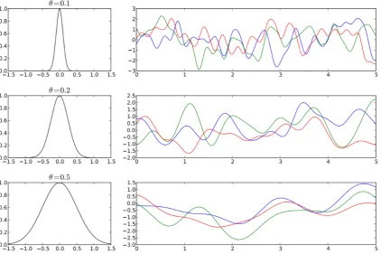
Figure 2.5:Samples from 1D GP priors with isotropic RBF kernel andθ=0.1, 0.2, 0.5. Left: the function
k(0,x). Right: the corresponding samples from the GP priors. (taken from [5]).
eters by providing 25 initial observations via successful demonstrated grasps (i.e. Kinesthetic learning) [16].
2.4 Acquisition Functions
The acquisition function is another component of Bayesian optimization where many design choices are available. The role of acquisition functions is to balance exploration and exploita-tion by providing a measure for the utility of obtaining a new observaexploita-tion at the pointxn+1 based on the surrogate model built using the past observationsD1:n. The next point to sample is then obtained by optimizing the acquisition function:
xn+1=arg max x∈χ α
(x|D1:n) (2.9)
The idea of Bayesian optimization is that, instead of optimizing an expensive black-box func-tion, a function that is relatively cheaper is optimized. In other words, the difficult original op-timization problem is solved by tackling an easier secondary opop-timization problem. Still, opti-mizing the acquisition function is not an easy task, especially in high dimensional spaces. Tech-niques used in literature to do this optimization range from random sampling, to discretiza-tion and adaptive grids. Multistarted quasi-Newton hill-climbing approaches can also be used when the gradient of the surrogate model is available or can be efficiently approximated [24]. Regardless of the taken approach, it is very difficult to ensure that the global maximum of the acquisition function was really found [24].
Figure 2.6:The shapes of three acquisition functions over a simple 1D GP posterior. (taken from [5])
As part of the flexibility of the Bayesian optimization framework, it is not necessary to stick to one hyperparameter value for the selected acquisition function. The value can be scheduled to change from one iteration to another. One of the popular schedules is to start with values that encourage exploration and then gradually move to a more exploitative behavior [5].
In fact, it is not even necessary to stick to one acquisition function throughout the optimization. Several techniques have been suggested to alter and mix between them [12].
2.4.1 Probability of Improvement (PI)
This function assesses, for a certain pointx, the probability of finding a target function value (or reward) that is higher than the maximum found observation by the hyperparameterξ:
P I(x)=P(f(x)≥max(y1:n)+ξ)=Φ
µµn(x)
−max(y1:n)−ξ
σn(x)
(2.10)
whereΦ(·) is the standard normal cumulative distribution function.
Maximizing theP I function results in selecting points most likely to offer an improvement of at leastξ. This allows ξto affect how local/global the search is. Ifξis very small, Bayesian optimization will be highly local and will not move to points far from the obtained observa-tion points before exhaustively investigating the area around the best observaobserva-tion so far. On the other hand, choosing a large value forξwill encourage more exploration and will prevent Bayesian optimization fromfine-tuning[5]. So, a middle point should be found.
Note that, because the fitted Gaussian process defines, at each pointx, a normal distribution
P(f(x)) over the value of f(x) at this point, Eq. 2.10 can be evaluated for any value ofξ.
2.4.2 Expected Improvement (EI)
This function assesses not only the probability of improvement when sampling at a certain pointx, but also the magnitude of this improvement.
CHAPTER 2. BAYESIAN OPTIMIZATION FRAMEWORK 15
whereσn(x)>0 (otherwise the function vanishes to zero),φ(·) is the standard normal proba-bility density function and
Z=µn(x)−max(y1:n)−ξ σn(x)
The full derivation of this function can be found in [24]. Here also the hyperparameterξhas a similar role as the one it has inP I: controlling the locality of the search.
2.4.3 Upper Confidence Bound (UCB)
This function simply gives higher values for points where the mean of the model is high as well as the uncertainty:
UC B(x)=µn(x)+κσn(x) (2.12) The hyperparameterκoffers a direct trade-off between exploration and exploitation. High val-ues ofκresult in exploring by selecting regions with high uncertainty. Low values ofκresults in exploiting by sticking to the regions where the mean is high.
2.5 Conclusion
After touching on the different parts of Bayesian optimization, it is important to relate back to our application of finding the optimal impedance parameters for an interactive drone. The design choices and assumptions done in this chapter are summarized here.
Considering the assumptions required by Bayesian optimization on the target black-box func-tion, it can be realized that they are not difficult to satisfy. First, the user has to provide the domain of the function. The simplest way of expressing the domain is as a hyper-rectangle in the space of impedance parameters values. In other word, the lower and upper bounds of each impedance parameter. Knowing that impedance parameters cannot take negative values as they result in controller’s instability, the lower bound is automatically provided. The upper bound is a little harder to determine as it is controller- and robot-specific. Based on the capa-bilities of the drone, the controller cannot be set on arbitrarily high gains.
The second assumption is that, within the given domain, the black-box reward function (per-formance measure) can be sampled at any location. Extra caution has to be taken concerning this assumption since, as mentioned in section 1.2, the parameter space of the impedance con-troller is not completely safe to explore and some locations within it lead to unstable behaviors. That is why the proposed learning framework in Fig 1.3 (section 1.3) contains a failure detec-tion block. The job of this block is to early detect if a certain selecdetec-tion led to instability, in which case it should immediately stop the current training episode, set the impedance parameters on some given safe default values, and send to Bayesian optimization a small reward (or a largely negative one) indicating that the performance was highly undesirable.
For the probabilistic surrogate model of Bayesian optimization, Gaussian processes were se-lected for their ability to naturally provide uncertainty measure over the whole target function domain allowing more effective exploration/exploitation trade-offs through acquisition func-tions and hence increasing the sample-efficiency of the technique.
The importance of providing meaningful initial knowledge was emphasized as it significantly affects the sample-efficiency of Bayesian optimization. Initial knowledge can be provided through the initial observations provided at the start of Bayesian optimization to build the ini-tial surrogate model. Carefully selecting the locations of these iniini-tial observations, the user can give hints to the learning algorithm that can make the task of finding high rewards easier.
RBF kernel is selected. Although this function builds a surrogate model that is infinitely differ-entiable (assuming that the target function is also infinitely differdiffer-entiable), this is unlikely to cause problems. It is important here to remember that the purpose of building the surrogate model is not to resemble the target function. The only important thing in the surrogate model is that the position of its global maximum converges to the position of the global maximum of the target function.
Regarding the selection of kernel hyperparameters values, it was explained that an isotropic kernel is used since we have no reason to believe that variation among one of the learned impedance parameters is more important than variations among the others. The exact values of the kernel hyperparameters are usually continuously adapted and inferred from the data at each Bayesian optimization iteration.
17
3 Bayesian Optimization Empirical Studies
In this chapter, Bayesian optimization is studied thoroughly by applying it to simulated black-box functions of different numbers of dimensions. The concentration is on the performance and behavior of the different acquisition functions and the effects of varying their hyperpa-rameters. The aim is to find settings that provide sample-efficiency and can scale to higher dimensions.
It was not possible to do this study directly on a simulated drone where the target function of Bayesian optimization is a black-box reward function calculated for a simulated impedance controller. This is because doing this study in a complete simulated environment would in fact take very long time for all the needed experiments to be finished (weeks of processing time). Additionally, this will make it difficult to generate various black-box functions as to generate a different black-box function, a new environment or a different task is needed.
To get around this, a software was written to generate random functions at any number of dimensions. The aim is not to produce functions that resemble the actual black-box reward functions encountered when working with the impedance controller of a drone, because this is practically impossible (otherwise, they are not black-box functions). Instead, the aim is to have a test bench that offers a relatively fast way of testing the different settings and seeing the
relativedifferences between them and across different numbers of dimensions.
[image:21.595.112.498.514.750.2]For easier navigation, Fig. 3.1 shows a roadmap of the chapter. The chapter starts with sec-tion 3.1 explaining the principles behind the software that generates random funcsec-tions. After that, section 3.2 presents the setup and conditions ensured throughout the experiments. It also discusses the important measures that should be monitored to assess the performance of Bayesian optimization. Then, section 3.3 presents and discusses the results of a parameter study over different acquisition functions in different dimensions. The insights gained from these results were used to propose a novel way of optimizing acquisition functions. The new method is explained in section 3.4 along with results showing its advantages. Section 3.5 (can be skipped) investigates an alternative automatic way of providing initial observations. Finally, the chapter is concluded with the main take-home lessons in section 3.6.
3.1 Generating Random Functions
As there are significant well-documented software contributions to Bayesian optimization [10, 4] and Gaussian processes [25], the idea was to generate random functions that represent an intuitively similar situation to the one that will be faced when dealing with the real black-box reward function. Then by applying Bayesian optimization on these functions, one can gain in-sights into various elements of the technique, like the acquisition functions and their hyperpa-rameters, the scalability to higher dimensions, the effect of the lack or presence of meaningful initial observations... etc.
The problem is, no ready solutions are available to do this task satisfactorily. So, a new module was written to do the job. The module is calledRandomFunctionand is written in Python. It will be released onGitHubas an open-source contribution to the research community. I explain here the main concepts of the used techniques, but refrain from discussing the code detailed implementation and leave that to the documentation included with the code.
The goal of the module is to produce a random functionSin any dimensiondgiven the domain (denotedχ) of the function as a list of closed intervals that form box boundaries in IRd, and the range (denotedR) as a closed interval.
3.1.1 Generating a Random Bell
Random functions are generated at any dimension with the help of the probability density function (PDF) of the multi-variate normal distribution. This function has the familiarbell
shape and is parameterized by the mean vector (determining the position of the center of the bell in IRd) and the covariance matrix (controlling the shape of the bell). It was chosen because it can be easily generated in any dimension. The module can generate a random bellbi:
bi(x)=
( 1
f(µi|µi,Σi)f(x|µi,Σi) ifx∈χ,
0 otherwise (3.1)
wheref is the PDF of the multivariate normal distribution,µi is the mean of the distribution chosen uniformly randomly from domainχandΣiis a randomly generated positive semi-def-inite convenience matrix with its elements kept within a range given by the user. Note that the PDF is normalized by dividing over its maximum (its value at the position of the mean).
Generating a random positive semi-definite matrix within a range of values given by the user was a challenging task. The current implementation relies on the fact that any matrix
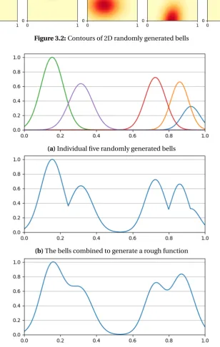
M=QTDQis a positive semi-definite matrix provided thatQis a full-rank matrix andDis a positive diagonal matrix. By selectingQto be random full-rank matrix with its diagonal ele-ments equal to zero, and selectingDas a random diagonal matrix, one can have separate con-trol on the range of values of the diagonal and off-diagonal elements of the covariance matrix, resulting on maximum control over the shape of the generated bells. Figure 3.2 shows ten 2D randomly generated bells. For these bells,χ={[0, 1], [0, 1]}, and the covariance diagonal range is [0.01, 0.05].
3.1.2 Forming a Random Function With Multiple Bells
Random functions of various shapes can be formed by combiningu (an integer given by the user) randomly generated bells. The module provides two ways of combining the bells. Both of them are illustrated on a simple 1D example in Fig 3.3.
The first way creates what we call aroughfunctionSrough:
Srough(x)=
hi max(h1:u)
CHAPTER 3. BAYESIAN OPTIMIZATION EMPIRICAL STUDIES 19
Figure 3.2:Contours of 2D randomly generated bells
(a)Individual five randomly generated bells
(b)The bells combined to generate a rough function
[image:23.595.145.454.214.702.2](c)The bells combined to generate a smooth function
wherehi is a scaling height selected uniformly randomly within [0, 1]. The function is nor-malized by dividing over the maximum height. One of the nice things about this function is that it is easy to locate its maximum, which is simply the mean of the bell associated with the maximum height max(h1:u). On the other hand, the first derivative of the resulting function is discontinuous at positions where two bells intersect as seen in Fig 3.3b.
The second way of forming a function creates asmoothfunctionSsmooth:
Ssmooth(x)=
1
Pu
i=1hibi(µm) u
X
i=1
hibi(x) (3.3)
wheremis the index of the bell corresponding to the maximum heightm=arg maxi∈[1:u]hi. The nice feature of smooth functions is that they are infinitely differentiable. However, the position of the maximum cannot be obtained analytically. It is not necessarily at the mean of the bell with the maximum heightµmsince the maximum of the sum of two Gaussians might be, in fact, somewhere between their means if they are close enough. With that in mind, the function in (3.3) is not completely normalized, but, intuitively, given that no other bell with the same height is close to the bell with the maximum height, the function maximum is very close to unity, and the position of the maximum is very close to µm. Providing bounds on the distance betweenµm and the global maximum as well as necessary conditions for these bounds requires a lengthy mathematical analysis and is beyond the scope of this report.
Notice that the generated (nearly) normalized functions can be easily scaled to match the func-tion rangeRgiven by the user.
One might intuitively think that the numberu of the bells that form a function determines the number of local maxima in that function. Looking to Fig 3.3, it can be seen that this is not true. The rough function constituted from five bells has only four local maxima, while the corresponding smooth one has only three. However, if the domain is large and the covariance of the randomly generated bells is chosen to be small, then controllingu directly determines the sparsity of the maxima over the function domain.
3.1.3 Alternatives and Advantages
A random function can also be generated at any number of dimensions by sampling it from a Gaussian process prior. This is because Gaussian processes provide probability distributions over the space of functions in IRd as seen in the previous chapter. However, one of the dis-advantages of this method compared to the method proposed here is that the position of the maximum cannot be easily located. Being able to locate the maximum of the generated func-tion is a key feature to allow clearer understanding of the behavior of Bayesian optimizafunc-tion when applied to that function.
More significantly, generating a random function by using a Gaussian process would make the Bayesian optimization experiments biased especially if the used Kernel in the GP used to gen-erate the function is the same as the one used in building the surrogate model in Bayesian optimization. Comparing equations (3.2) and (3.3) of the rough and smooth functions with the the equation of the GP prior (2.3), and also the shapes of the generated functions (Fig. 3.3) with those of the GP priors with the RBF kernel (Fig. 2.5), it can be clearly seen that the generated functions according to the described methods are totally different than those generated by GP priors. One of the clear differences is that, compared to GP priors, the generated random func-tions characteristics are not controlled by a kernel at all and so can be varying rapidly in one area but varying very slowly in another one. Hence, the proposed method does not suffer from this bias problem.
CHAPTER 3. BAYESIAN OPTIMIZATION EMPIRICAL STUDIES 21
graphs, 2D contours or 3D surfaces for the generated random function or a cross-section of it (ifd>2).
3.2 Experimental Setup
To ensure the meaningfulness of the Bayesian optimization simulations performed on the ran-domly generated functions, some initial conditions and settings were kept throughout gener-ating all the results seen in next suctions.
3.2.1 Random Functions Settings
All the experiments shown in this chapter were done over ten1randomly generated functions per number of dimensions. The group of functions were generated once and kept throughout the experiments to produce comparable results. The measurements taken during these exper-iments were averaged over the ten functions. Figure 3.4 shows the ten 2D randomly generated functions used in the experiments.
Figure 3.4:Contours of ten 2D randomly generated smooth functions. Darker areas have higher values (rewards).
All the functions were generated with a domain that forms a unit hyper-cube in IRd. The range of the functions was kept [0, 1]. Because sooth functions cannot be completely normal-ized since the position of the maximum cannot be determined analytically as mention in sec-tion 3.1, it is not possible to ensure that the maximum of the generated smooth funcsec-tions is one. In fact, by doing a grid search (0.001 precise) on the ten used 2D functions, it was found that the average of their global maxima is 1.04. All the experiments were performed on smooth functions unless otherwise mentioned. This is because, for our application that involves work-ing with dynamic robotic systems, we do not expect the black-box reward function that will be optimized to have a discontinuous derivative.
The numberuof bells per function was selected to be 30 for all numbers of dimensions. The range of the values of the diagonal elements of the covariance matrix was also selected to be the same for the functions generated in all numbers of dimensions. This is to ensure similar variations among the functions generated in different numbers of dimensions. This range was selected to be [0.005, 0.01]. This generates small bells to allow functions with various complex
1Doing an experiment for 10 functions is already computationally expensive. It can take up to 40 minutes to
shapes as in Fig 3.4. It is easy to imagine functions with similar shapes being encountered when optimizing the reward function of the drone’s interaction controller.
3.2.2 Bayesian Optimization Software and Settings
At an early stage of the research, I implemented Bayesian optimization following the algorithm described in [16]. The implementation contained a simple Gaussian process inference with the squared exponential kernel. The UCB acquisition function was used and was optimized using gradient decent with a variable learning rate. The implementation was intended to understand the technique and explore its various elements. However, expectedly, readily available open-source packages offer more efficiency and flexibility.
Two packages were investigated and the decision at the end was in favor of using
BayesianOptimization[10] over the olderGPyOpt[4]. What makes the selected package appealing is the clarity and simplicity of its implementation and documentation, allowing easy modification and development in the different parts of the Bayesian optimization frame-work. This feature was exploited when introducing a novel method for optimizing acquisition functions as will be seen in section 3.4.
In addition, the package is built over scikit-learn’s Gaussian processes modules [25], which offers a wide range of kernels and, more importantly, the possibility to optimize the ker-nel hyperparameters through multiple-seeded maximization of the marginal likelihood of the obtained models (as mentioned in section 2.3.1).
All the experiments shown in this chapter are done with ten random initial observations to gen-erate the initial model (line 1 of Algorithm 1). For each randomly gengen-erated function, ten ran-dom points are chosen uniformly ranran-domly within the ran-domain of the function and are main-tained to be used in all experiments where this random function is used. This ensures that results of experiments done for different settings are comparable as the initialization is always the same. After these ten initial observations, Bayesian optimization runs for another forty iter-ations, meaning that the function will be propped for a total of fifty times. This is done because the interest is in finding sample-efficient techniques.
As decided in section 2.3.1, the RBF kernel is used. During each iteration of Bayesian opti-mization, thescikit-learn’s Gaussian process module is set to optimize the kernel hyper-parameterθwhen building a posterior over the observations received so far (line 3 of Algo-rithm 1). The module is set to randomly seed the optimization 25 times to find the best value for the hyperparameter. This is of great help to the user of Bayesian optimization as it takes away the burden to set these very significant hyperparameters.
As we expect no noise in these randomly generated functions, theσ2 hyperparameter seen in equations (2.4), (2.6) and (2.7) was set to 10−5. According to the documentation of the
scikit-learnpackage [25], even in the presence of no noise, it is useful to set this param-eter to a value slightly greater than zero to ease some numerical issues faced during Gaussian process fitting. The value of the hyperparameter should be increased depending on the antici-pated noise in the observations of the real black-box function.
CHAPTER 3. BAYESIAN OPTIMIZATION EMPIRICAL STUDIES 23
3.2.3 Measures for Assessing Optimization Performance
From the author’s point of view, three measures are of special importance to the understanding of Bayesian optimization performance:
• y+
n: the maximum obtained reward so far
y+n=maxy1:n (3.4)
• ¯yn: the average of all obtained rewards so far
¯
yn= n
X
i=1
yi/n (3.5)
• dn: the Euclidean distance between the position of the current observation and the clos-est past observation
dn=min{pxn−xi}ni=−11 (3.6) The graph ofyn+corresponds to the learning rate graph in classical reinforcement learning liter-ature. It shows how fast the optimization found the position of the maximum. Ify+n is increas-ing with the number of iterationsn, then a new maximum is found every iteration, else, if it stays constant, then no new maximum has been found since the last increase (positive slope). Clearly,yn+cannot decrease with time.
Looking at the curve of ¯yngives an indication if the optimization method is constantly trying at areas of low reward, which will make ¯yndecrease with time. In other words, ¯yncan be used as a safety measure of the learning considering that falling to areas of low rewards, when dealing with the impedance controller’s black-box reward function, corresponds to bad or dangerous performance during performing the predetermined task.
Finally,dn can be used to see how local/global the search is. If dn is high for a number of iterations, then the search is constantly looking to positions that are far from already seen ob-servations.
It is important to emphasize that these measures, shown in the coming figures, are averaged over experiments performed for ten different randomly generated functions as mentioned in section 3.2.1.
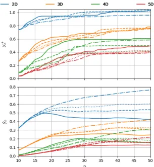
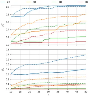
3.3 Parameter Study of Acquisition Functions
In this section, an empirical parameter study is done over the three acquisition functions dis-cussed in section 2.4. Two main questions are of special importance:
1. How does changing the hyperparameters of the acquisition functions affect the learning performance and the exploration/exploitation trade-off?
2. how do acquisition functions settings scale with higher number of dimensions?
To isolate the effect of changing the hyperparameters values, it is studied and compared over 2D functions in subsection 3.3.1. To make sure that the observations and conclusions reached in 2D still apply as the number of dimensions increases, the same experiments are repeated for 3D functions in subsection 3.3.2. Then, to investigate more the effect of increasing the number of dimensions of the learning problem, the experiments results are presented and compared over four different numbers of dimensions in subsection 3.3.3.
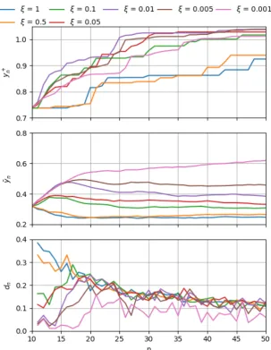
3.3.1 Acquisition Functions in 2D PI Results
Figure 3.5 shows the three measures mentioned above for the PI acquisition function with a range of values for its hyperparameterξover ten randomly generated 2D functions. Looking at the topyn+graph, it can be seen that for high values ofξ(more exploration) the maximum value reached by the end of the 50 observations is low with respect to values reached by other settings. This is due to the fact that more global searches cannot properly fine-tune to reach the position of the maximum. On the other hand, very small values ofξ(0.001 on the extreme) slow down the search. It can be noticed that a middle value of 0.01 produces the best result in this case, with a curve that quickly reaches a high value.
Figure 3.5:Performance of PI with different values forξover 2D functions.
Observing the middle ¯yn graph, another interesting trend can be noticed. Bayesian optimiza-tion with more local acquisioptimiza-tion funcoptimiza-tion (low values ofξ) accumulates a greater average reward over time even though it might have not necessarily reached the postilion of the maximum re-ward. This is understandable, since more local search have a lower risk of falling into areas of smaller rewards than what was already obtained.
CHAPTER 3. BAYESIAN OPTIMIZATION EMPIRICAL STUDIES 25
with very high rewards. Instead, at every iteration, the maximum of the acquisition function with nearly all values ofξis about 0.1 away from the closest seen observation.
EI Results
Figure 3.6 shows the performance of the EI function. All of the observations mentioned for the PI function can be repeated here with few exceptions. While higher values ofξstill leads to bad
yn+curves, performance improves asξdecreases. In fact, the besty+n curve is that of the lowest value ofξ. However, it should be noted that theyn+curves of EI need more iterations to start going up than those of PI. It is also clear that the ¯yncurves of PI are generally much higher than those of EI. On the other hand, thedncurves of both functions are very similar.
Figure 3.6:Performance of EI with different values forξover 2D functions
UCB Results
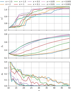
In Fig. 3.7, the performance of Bayesian optimization with the UCB function is shown. It can be seen that for the higher values ofκ,yn+increases slowly with time. For the lowest values ofκ, however, the search quickly converges to a local maximum and starts exploiting it (hence the horizontal line at the end).
For thedn curves, similar to PI and EI, UCB with lower values ofκstarts exploring locations closer to the already seen observations. Unlike PI and EI, on the other hand, as the number of iterations increases, thedn gradually decreases reaching around zero at the end for all values ofκ.
Figure 3.7:Performance of UCB with different values forκover 2D functions
Discussion
Considering the shown results, it should be emphasized that the objective of Bayesian opti-mization is not to maximize ¯yn, buty+n. So a method that quickly finds highery+n while getting a lower ¯yn(because it occasionally falls into areas of smaller rewards while exploring) is favor-able (observe they+n and ¯yncurves for PI withξ=0.01). However, methods that can do both tasks are very desirable, especially for a cost- and safety-critical system like the dynamic robotic system we are dealing with here. Finding a Bayesian optimization configuration that can main-tain an increasingyn+and ¯ynduring the learning, actually means that the robot (drone) will be less probable to fall into areas of bad performance or, worse, instability.
CHAPTER 3. BAYESIAN OPTIMIZATION EMPIRICAL STUDIES 27
those of UCB as continuous exploration leads to higher chances of occasionally getting lower rewards.
It is interesting to see that, unlike PI and EI, for lowest values of its hyperparameterκ, UCB doesn’t fine-tune and reach highery+n. Instead it begins exploiting quickly around a relatively low reward. What happens is that when the surrogate model evolves to a situation where the sum of the mean and the weighted variance of the model (as in Eq. (2.12)) are smaller than the currentyn+, the maximum of UCB will be always at the location ofy+n or locations that are very close to it anddnwill converge to zero. This happens early for low values ofκresulting in an earlier exploitative behavior. This in turn results in higher steadily increasing ¯yncurves.
Choosing higher values forκdelays this exploitative behavior, allowing the search to explore more positions and preventing it from easily falling in local maxima. However, it results in a lower ¯yn curves due to the increased risk of falling in areas of low rewards because of explo-ration.
A very important insight here is that, while PI and EI manage exploration and exploitation indi-rectly by controlling the desired improvement, UCB diindi-rectly balance exploration and exploita-tion and hence is able to stop looking further when ‘satisfied’. This makes the ¯yncurves of UCB (even for the high values ofκ) the highest among the three functions. However, because UCB sooner or later stops exploration, it is generally more probable to get stuck in a local maximum.
Looking at the performance of three functions in the 2D case, it can be concluded that PI is more capable of reaching the maximumyn+and UCB has the lowest probability of falling into areas of low rewards (hence has high ¯yn curves). The performance of EI in both criteria is inferior. It is important to investigate if these findings hold for higher numbers of dimensions.
3.3.2 Scaling up to 3D
Figures 3.8, 3.9 and 3.10 show the behavior of PI, EI and UCB respectively on 3D functions for a range of settings. One note to begin with is that the averages of the maximum rewardy10+ and the mean reward ¯y10during initialization are much lower that these of the 2D functions. This is because of the increased sparsity due to the added dimension making it harder for random initial points to pick potions of high rewards.
y10+ can be considered the ‘initial knowledge’ the optimization algorithm has about the value and the corresponding position of the maximum. It can be seen that with this small initial knowledge, there was no way of reaching the global maximum (whose value is slightly higher than 1.0) with 10 initial observations and another 40 Bayesian optimization iterations. Note thaty10+ and ¯y10are always that same regardless of the setting. This is because every randomly generated function has its own set of random initial points that is retained throughout the ex-periments as explained in section 3.2.2.
PI Results
Looking to Fig. 3.8, the same PI curves trends foryn+, ¯yn anddn curves seen in the 2D case can be seen here. However, in the case of 3D functions, we find that the setting leading to the highesty+
n, is the same as the one with the highest ¯yncurve and is the smallest value (ξ=0.001). This raises the concern that the optimal setting can be different depending on the number of dimensions of the black-box function, and brings the natural question: how can one determine the optimal setting?
Figure 3.8:Performance of PI with different values forξover 3D functions
that decide to learn each of the spring parameters individually, which converts the problem to a 6D one although we are still working with the same dynamic system. What this observa-tion says is that the user might need to change the settings of the acquisiobserva-tion funcobserva-tion or use a completely different one.
Notice that these issues are only significant due to the limited number of allowed black-box function observations (again due to the high cost of a single observation). In problems where hundreds or thousands of observations are allowed, these issues are not of great influence, and hence are not often tackled in literature.
CHAPTER 3. BAYESIAN OPTIMIZATION EMPIRICAL STUDIES 29
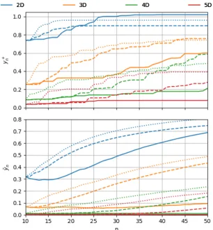
Figure 3.9:Performance of EI with different values forξover 3D functions
EI Results
The performance of EI (Fig. 3.9) deteriorates more with one higher number of dimensions. The function is much slower than the other two in reaching highyn+values and also has, by far, the lowest ¯yn curves. This clearly indicates that EI is not suitable for sample-critical situations. It needs a higher number of observations for its merits to be seen, which makes it unsuitable for the application at hand.
UCB Results
![Figure 2.6: The shapes of three acquisition functions over a simple 1D GP posterior. (taken from [5])](https://thumb-us.123doks.com/thumbv2/123dok_us/9690311.470376/18.595.117.454.79.354/figure-shapes-acquisition-functions-simple-gp-posterior-taken.webp)