Testing for spatial heterogeneity in functional MRI using the multivariate general linear model

University of Warwick institutional repository: http://go.warwick.ac.uk/wrap

This paper is made available online in accordance with publisher policies. Please scroll down to view the document itself. Please refer to the repository record for this item and our policy information available from the repository home page for further information.

To see the final version of this paper please visit the publisher’s website. Access to the published version may require a subscription.

Author(s): Robert Leech and Dennis Leech

Article Title: Testing for spatial heterogeneity in functional MRI using the multivariate general linear model

Year of publication: 2010 Link to published article:

http://www2.warwick.ac.uk/fac/soc/economics/research/workingpapers/ 2010/twerp_938.pdf

Testing for spatial heterogeneity in functional MRI using the

multivariate general linear model

Robert Leech and Dennis Leech

No 938

WARWICK ECONOMIC RESEARCH PAPERS

Testing for spatial heterogeneity in functional

MRI using the multivariate general linear model

Robert Leech

and Dennis Leech

1

_{The Computational, Cognitive and Clinical Neuroimaging}

Laboratory, The Division of Experimental Medicine, Imperial

College London, Hammersmith Hospital Campus, Du Cane

Road, London, W12 0NN, UK

2

_{Department of Economics, University of Warwick, Coventry,}

1

Abstract

Much current research in functional MRI employs multivariate machine

learn-ing approaches (e.g., support vector machines) to detect fine-scale spatial

pat-terns from the temporal fluctuations of the neural signal. The aim of many

studies is not classification, however, but investigation of multivariate spatial

patterns, which pattern classifiers detect only indirectly. Here we propose a

direct statistical measure for the existence of fine-scale spatial patterns (or

spatial heterogeneity) applicable for fMRI datasets. We extend the univariate

general linear model (typically used in fMRI analysis) to a multivariate case.

We demonstrate that contrasting maximum likelihood estimations of

differ-ent restrictions on this multivariate model can be used to estimate the extdiffer-ent

of spatial heterogeneity in fMRI data. Under asymptotic assumptions

infer-ence can be made with referinfer-ence to the χ2 _{distribution. The test statistic is}

then assessed using simulated timecourses derived from real fMRI data. This

demonstrates the utility of the proposed measure of heterogeneity as well as

considerations in its application. Measuring spatial heterogeneity in fMRI has

important theoretical implications in its own right and has potential uses for

better characterising neurological conditions such as stroke and Alzheimer’s

Key wordsNeuroimaging, Multivariate pattern analysis, Maximum

likeli-hood estimation, Seemingly unrelated regression.

2

Introduction

The traditional approach to quantifying changes in brain activation with

func-tional magnetic resonance imaging (fMRI) is massively univariate; a separate

general linear model is fitted to the time series of each of the many tens of

thousands of spatially distinct measurement locations (voxels). Given the

rel-atively poor signal-to-noise of the measurable signal, Gaussian spatial

smooth-ing across neighborsmooth-ing voxels is normally applied. However, this smoothsmooth-ing

assumes that the detectable neural signal is spatially homogeneous (i.e.,

ap-proximately the same general linear model should fit adjacent voxels). This

assumption has been the subject of intense recent debate (de Beeck and Hans

2009, Kamitani and Sawahata 2009, de Beeck and Hans 2010). Some

multi-voxel analysis techniques indicate that brain regions may be highly

heteroge-neous (Haxby et al. 2001, Kamitani and Tong 2005, Haynes et al. 2007) and

uni-variate approach. Furthermore, whether areas of the brain are highly

heteroge-neous (with find-scale spatial pattern information) is important theoretically

for understanding the roles of regions of cortex, with potential implications

for better understanding neurological conditions such as Alzheimer’s disease

or stroke. However, the multivariate pattern classification techniques used to

date (e.g., support vector machines and linear discriminant analysis) are

indi-rect ways to measure the heterogeneity of the fMRI signal across brain regions.

In this paper, we propose a framework and test statistic to directly measure

the extent to which there is a heterogeneous pattern of activation across

neigh-boring voxels. The proposal takes as it’s starting point the information-based

approach of Kriegeskorte and colleagues (Kriegeskorte et al. 2006a). Instead

of using multivoxel pattern classifiers to decode which state the brain is in

as a proxy for the amount of information available in a region,

Kriegesko-rte and colleagues proposed using a variant on the Mahalanobis Distance to

provide a measure of the amount of information available across voxels in a

patch of cortex. The Mahalanobis distance statistic wasshown to be

substan-tially more sensitive at detecting signals than standard univariate t-statistics

suc-cessfully in several fMRI experiments within the visual domain (Kriegeskorte

et al. 2006a, Serences and Boynton 2007a;b, Stokes et al. 2009).

The Mahalanobis distance (Mahalanobis 1936) is a multivoxel similarity

measurement that unlike Euclidean distance is scale invariant and controls

for covariance across datapoints. In fMRI datasets, the Mahalanobis distance

can calculate the similarity between different experiment conditions, e.g., how

dissimilar are visual and auditory processing for a given set of voxels. This

statistic controls for error covariance across voxels; spatially correlated error is

expected in fMRI datasets given spatial patterns of sources of noise affecting

the BOLD signal, such as vasculature, movement artifacts etc. To calculate

the Mahalanobis distance, Kriegeskorte et al. (2006b) fitted a separate GLM

analysis to the unsmoothed functional data for each voxel. The Mahalanobis

distance was then calculated using the resulting vectors of beta weights and

the residual error covariance matrix across voxels

with two types of stimuli andΣˆ is the error covariance matrix.

In this paper we start by demonstrating how the Mahalanobis distance

re-lates to the mulrivariate general linear model. We then set up different

restric-tions on the GLM to compare models under an assumption of spatial

homo-geneity and spatial hetereogenity resulting in a chi-square statistic measuring

the heterogeneity in a patch of cortex. This statistic explains the amount of

fine-scale information available across a number of voxels. The statistic is then

assessed with synthetic data derived from fMRI datasets to demonstrate its

utility and to explore limitations in its application.

3

Theory

3.1

The statistical model

We start with the GLM as applied to fMRI datasets (Friston et al. 1994).

We assume the response by each voxel can be modelled by a linear regression

yit= k !

h=1

βhixht+uit (2)

where i is the voxel subscript, i = 1, ..., n, and t is the time subscript, t =

1, ..., T. βhi represents the response of voxel i to the stimulus measured by

regressor h.

This can be written using matrix algebra as,

yi =Xβi +ui (3)

where yi is the T element observation vector for voxel i, X the Txk input

matrix, ui the T element error vector, and βi the k element coefficient

vec-tor. There is a different regression model for each voxel but all models have a

common regressor matrix.

The error for each voxel equation is assumed to have zero mean, be

seri-ally independent and homoscedastic, but correlated across equations. That is,

E(ui) =0 for all i and E(uiu!j) = σijIT for all i and j.

This system of equations can be written more compactly as:

where y=             y1 y2 ... yn            

, u =

            u1 u2 ... un            

, β=

            β1 β2 ... βn            

, Z =

           

X 0 . . . 0

0 X . . . 0

... ... ... ...

0 0 . . . X

           

=In⊗X,

Ω=            

σ11IT σ12IT . . . σ1nIT σ12IT σ22IT . . . σ2nIT

... ... . .. ...

σ1nIT σ2nIT . . . σnnIT            

=Σ_⊗IT, and Σ=            

σ11 σ12 · · · σ1n

σ12 σ22 · · · σ2n

... ... ... ...

σ1n σ2n · · · σnn             .

It is well known (for example (Zellner 1962, Greene 2003)) that, when there

is a common set of regressors, the correlation of the errors in different equations

is irrelevant to coefficient estimation. The efficient estimator, equivalent to

generalized least squares, is ordinary least squares applied to each equation

separately. That is, the efficient estimator of the complete system is written:

ˆ

βi =(X!X)−1X!yi, for all i, and thereforeβˆ=(Z!Z)−1Z!y. (5)

The covariance matrix of βˆcan be shown to be

Noting that

Z!Z = [In⊗X!][In⊗X] =In⊗X!X, and hence that (Z!Z)−1 =In⊗(X!X)−1,

and that

Z!ΩZ = [In⊗X!][Σ⊗IT][In⊗X] =Σ⊗(X!X),

we can rewrite (6) as

V(βˆ) = [In⊗(X!X)−1][Σ⊗(X!X)][In⊗(X!X)−1] =Σ⊗(X!X)−1. (7)

This gives a simple expression for the covariance between any pair of

esti-mated coefficients. Letting W = (X!X)−1_{, we can write}

Cov( ˆβgi,βˆhj) = σijwgh (8)

for all pairs of voxels i, j = 1, ..., n, and all pairs of regression coefficients

g, h= 1, ..., k.

All this assumes that the covariance matrix of equation errors,Σ, is known.

In practice it must be estimated consistently from the residuals, using,

ˆ

σij = (yi−Xβˆi)!(yj −Xβˆj)/T, (9)

(or, ˆσij = (yi−Xβˆi)!(yj−Xβˆj)/(T−k)) and Σreplaced with ˆΣthroughout

3.2

Inference

Our focus is on testing a set of linear restrictions on coefficients across the

separate voxel equations. We assume there are g restrictions written in the

form Rβ= 0 where R is a g×nk matrix of given constants of rank g. (We do not need to consider inhomogeneous restrictions here because units of

mea-surement are arbitrary in the context.)

This framework allows us to devise tests for heterogeneity versus

homo-geneity (that is, constancy) of the effects of different stimulae across voxels,

as well as to test if stimulae are significantly different from zero.

If the equation errors uit are Gaussian then the efficient estimator of β

given in equation (5) is normally distributed and the well known (see for

ex-ample Rao 1973) inferential procedures for generalized linear regression models

are available based on the covariance matrix in equation (6), (7) or (8). These

hold asymptotically if Σis estimated consistently.

general type

H0 :Rβ= 0. (10)

which can be approached in various ways, for example by a Wald or LR

prin-ciple.

Letting Rβ = δ the null hypothesis of interest becomes H0 : δ = 0.

Now define δˆ = Rβˆ. Then δˆ is asymptotically normally distributed with expectationE(δˆ) = 0and covariance matrixV(δˆ) =RV( ˆβ)R!. We call the test statistic ∆, given by

∆ =δˆ![RV( ˆβ)R!]−1δˆ (11) which has an asymptoticχ2_{distribution withg degrees of freedom ifH}

0 is true.

Alternatively we employ the likelihood principle and LR tests based on the

loglikelihood function

lnL=−T n

2 ln(2π)−

T

2ln|Ω| − 1

2Q (12)

whereQ is the appropriate generalized sum of squared residuals,

We can specify a LR test of a null hypothesis in the form of (10) as twice the

difference between the maximized value of (12) under the null and alternate

hypotheses, LR=−2(lnL0−lnL1). The test statistic is then

LR=Q0−Q1, (14)

whereQ0is the minimum of (13) underH0andQ1the unconstrained minimum

(or, the minimum under the alternateH1). This assumesΣto be known or the

same estimate of it used under both the null and alternate. Standard theory

gives the statistic (14) an asymptotic chi-squared distribution with g degrees

of freedom. (See (Greene 2003).)

3.3

Testing heterogeneity across voxels

We now describe tests of spatial characteristics of the multivariate signal across

voxels. In particular, we are interested in investigating heterogeneity of

re-sponse coefficients. We describe a procedure for comparing the unrestricted

model, allowing heterogeneity between voxels, with a restricted model, which

we say has homogeneity between voxels.

We characterize the null hypothesis of homogeneity in terms of a linear

r!_β

i for suitable constants r! = (r1, r2,· · · , rk). The null hypothesis states

thatr!_β

i is constant for alli. That is,r!βi =r!βj for alli$=j. Therefore, we

can write the restrictions to be tested in the form: H0 :Rβ=0

with R=            

r! _−r! ₀! _{· · · 0}!

r! 0! −r! · · · 0!

... ... ... ... ...

r! ₀! ₀! _{· · · −r}!

            .

An important case is where interest centers on the difference between two

effects. If the two effects are assumed to be the first two coefficients, then

r!βi =β1i−β2i and r! = (1,−1,0,· · ·0).

Let the common difference be θ. Then the restricted model can be written

H0 :β1i−β2i =θ, constant for all i.

βs). Under the restrictions inH0 there are nk−n+ 1 coefficients (thenk β’s

less the n β2’s plus θ). Therefore the number of parameter restrictions under

H0 is n−1.

The LR test requires estimating the model, and evaluating the log

likeli-hood, separately underH1andH0. We proceed as ifΣis known; it is estimated

from the residuals of the unrestricted model. The unrestricted model is

effi-ciently estimated as a set of ordinary least squares regressions. The restricted

model can be estimated using a simple reparameterization as follows.

Write β1i =β2i+ (β1i−β2i). Under H0, this becomes β1i =β2i +θ.

Substituting into (2) and collecting terms in β2i gives the restricted set of

equations,

yit =θx1t+β2i(x1t+x2t) + k !

h=3

βhixht+uit (15)

The system of equations (15) is a set of seemingly unrelated regressions

with a common set of regressors (a multivariate regression) with cross-equation

y =θx˜+ ˜Zγ+u, (16) where we define

γ=             γ1 γ2 ... γn            

,γi =            

β2i

β3i

... βki            

, i= 1, ..., n, and ˜Z =

            ˜

X 0 . . . 0

0 X˜ . . . 0

... ... ... ...

0 0 . . . X˜

           

=In⊗X˜,

˜

X is the T(k ₋1) matrix, ˜X = [x1 +x2,x3, . . . ,xk], where xi is the ith

column of the design matrixX,

and ˜x=

            x1 x1 ... x1            

=ιn⊗x1,where =ιn=             1 1 ... 1             .

We can rewrite the system

y−θx˜ = ˜Zγ+u, (17) which can also be written,

a system with common regressor set for given θ, and therefore the γis are

estimated efficiently by OLS applied separately to each equation.

This is equivalent to estimating (17) by ordinary least squares giving,

ˆ

γ= ( ˜Z!Z˜)−1Z˜!(y₋θx˜). (18) which is the maximum likelihood estimator of γ conditional on θ.

The likelihood function (12) is maximized when the generalized least squares

criterion (13) is minimized. Write,

Q(θ,γ) = u!Ω−1u= (y−θx˜−Zγ˜ )!Ω−1(y−θx˜−Zγ˜ ).

Substituting (18) forγ in this, we concentrate the generalized sum of squared residuals function (13) with respect to γ and obtain a function of θ only, say

Q∗(θ):

Q∗(θ) = [y₋θx˜₋Z˜( ˜Z!Z˜)−1Z˜!y₋θZ˜( ˜Z!Z˜)−1Z˜!x˜]!Ω−1[. . .].

If we writeM =I₋Z˜( ˜Z!Z˜)−1_Z˜!_{, we can define y}r _{=M y, and ˜x}r _=Mx˜

Hence,

Q∗(θ) = [yr₋θx˜r]!Ω−1[yr₋θx˜r], (19) which is minimized by the maximum likelihood estimator.

The estimator ofθ, which minimizes (19), and is also the ML estimator, is

easily shown to be found by a bivariate generalized least squares regression of

yr _{on ˜x}r_{, giving:}

ˆ

θ= x˜

r!_Ω−1_yr

˜

xr!_Ω−1_x˜r. (20)

The LR criterion (14) is then simply evaluated.

4

Simulations

To test the proposed log-likelihood-ratio measure of heterogenity, we applied

it to simulated data generated from an fMRI dataset. Using synthetic data

allowed us to: (1) systematically vary the spatial characteristics of the

sig-nal; (2) test the validity of the asymptotic chi-square distribution of the test

statistic under different conditions (i.e., with different numbers of voxels and

timepoints); and (3) investigate violations of the assumptions of the GLM, i.e.,

FMRI data was taken from a 32-year-old neurologically healthy male

par-ticipant who provided informed consent according to local ethics procedures.

Two-hundred and seventy-six echoplanar images of resting data (i.e., the

par-ticipant lay in the scanner doing nothing) were acquired (i.e., 276 timepoints

at each voxel) with a resolution of 2.19_× 2.19_×4.0 mm. The covariance

ma-trix across neighboring voxels (chosen from within superior temporal cortex)

was calculated. This covariance matrix was used to generate random noise

sampled from a multivariate normal distribution.

4.1

Simulating spatial heterogeneity

In the first set of simulations, we demonstrate that the test statistic has power

with respect to multivariate heterogeneity. A design matrix was constructed

with three columns (k=3), consisting of two dichotomous variablesx1t andx2t

and a constant x3t. At each timepoint either x1t= 1 (and x2t= 0) or x2t= 1

(and x1t = 0). For a third of timepoints, both x1t = 0 and x2t = 0. In the

first case, seven timeseries (this corresponds to a central voxel and adjacent

voxels) were generated by drawing 276 timepoints from a multivariate normal

β values was added to the random noise. In the homogeneous case, all seven timeseries had the same signal (i.e., the betas associated with experimental

condition one were either positive in all voxels or negative in all voxels). In

the heterogenous case, half of the timeseries had positive β) values for condi-tion one and half had negative beta values. Note the overall signal was the

same in all situations (i.e., the absolute difference between condition 1 and

condition 2 was constant).

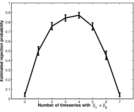
Figure 1 shows the results of 500 simulations with different covariance

ma-trices and randomly generated timeseries. The x-axis represents the number

of timeseries with homogeneous signals. As the number of timeseries with

β1 positive and β2 negative increases the heterogeneity across the timeseries

increases. This is reflected in the increase in the estimated rejection

proba-bility. As such, the test statistic reflects the degree of heterogeneity in the β

coefficients across the timeseries.

4.2

Asymptotic

χ

assumption

The χ2 _{properties of the test statistic only hold asymptotically, and previous}

0 1 2 3 4 5 6 7 0

0.1 0.2 0.3 0.4 0.5 0.6 0.7 0.8 0.9 1

Estimated rejection probability

Number of timeseries with β 1 > β2

Figure 1: Varying heterogeneity across the seven timeseries. At the extreme

values of the x-axis all timeseries (voxels) have the same β) coefficients: the homogeneous cases. In the center of the x-axis, half the voxels have β1) >

β2) and half the reverse. The y-axis is the log-likelihood ratio comparing

the unrestricted and restricted models. The dotted line marks the χ2 _{value of}

p<0.05. Mean and standard error of the estimated rejection probability across

as the covariance matrix increases in size, this assumption becomes untenable

except with very large numbers of timepoints. With smaller numbers of

time-points, overrejection of the null hypothesis becomes an issue.

We investigated the validity of theχ2 _{assumption in two situations: 1) one}

with 7 timeseries (equivalent to a sphere of 1 voxel radius around a central

voxel); and 2) one with 33 timeseries (equivalent to a sphere of 2 voxel radius).

In both situations, multivariate random noise was generated with a real

co-variance structure. Since we are interested in the assessing the overrejection

rate of estimated χ2 _{values, no signal was inserted into the background noise.}

The number of timepoints was varied in from 50 to 1500, and a hundred

sim-ulations and models were fitted with each number of timepoints.

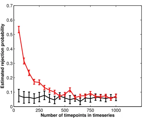
Figure 2 shows the proportion of models that are judged to be significant

at a p<0.05 significance level. Given the absence of signal, this value should

be approximately 0.05. We see that for the seven timeseries case, there is not

substantial overrejection of the null hypothesis, even with only 50 timepoints.

However, for the larger 33 timeseries scenario, incorrect overrejection of the

0 250 500 750 1000 0

0.1 0.2 0.3 0.4 0.5 0.6 0.7

Number of timepoints in timeseries

Estimated rejection probability

Figure 2: The proportion of models that incorrectly reject the null hypothesis

assuming the difference in log likelihoods isχ2_{distributed for different numbers}

of timepoints. The red line is the case with 33 timeseries and the blue line

with 7 timeseries. Values are the mean and standard error of 500 simulations.

null occurs half the time. Only after approximately 500 timepoints does the

rejection rate approximate that expected given the null hypothesis. This

find-ing highlights the problem of accurately estimatfind-ing large covariance matrices

without large numbers of datapoints. In these situations, the log-likelihood

4.3

Autocorrelation of the residuals

One common problem in applying the GLM to fMRI timeseries is the presence

of autocorrelation in the residuals. In general, this can lead to underestimation

of the error variance and inefficient model estimation. We conducted

simula-tions to investigate the effects of error autocorrelation on the proposed

log-likelihood ratio statistic. Fifteen-order autocorrelation estimates were

calcu-lated using standard analysis software fsl (Woolrich et al. 2001). Multivariate

normally-distributed random data was then filtered using these

autocorrela-tion estimates to simulate realistic autocorrelaautocorrela-tion in an fMRI dataset. Two

situations were considered: one with a rapidly varying design matrix (with

timepoints assigned to either condition one or condition two intermixed at

random; equivalent to an event-related fMRI experimental design). The

sec-ond was equivalent to a blocked fMRI design, with a continuous sequence of

timepoints (one third of the total) corresponding to one condition, followed by

another third corresponding to the other condition.

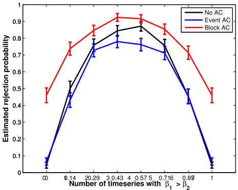
Figure 3 shows the performance of the blocked and the event-related

ex-perimental design in the presence of autocorrelation of the residuals. Inflation

design was similar (slightly more conservative) than a model with no

autocor-relation. This result highlights that correction of autocorrelated noise is an

important step for the proposed statistic (as for many fMRI analyses),

espe-cially for blocked experimental designs. Standard techniques for prewhitening

(Woolrich et al. 2001) non-white noise can be used in conjunction with the

statistics proposed here.

5

Discussion

In this paper, we have presented a measure of multivariate heterogeneity across

multiple timeseries, that is designed to be able to assess the amount of

mul-tivoxel information available in functional MRI datasets. We extended the

univariate GLM to a multivariate case, an example of seemingly unrelated

re-gression, equivalent to a Mahalanobis distance measure previously used with

fMRI. An unrestricted version of the multivariate GLM provides the maximum

likelihood model across timeseries (allowing β values to be different for each timeseries). A restricted model assessed the homogeneous case that all

0 1 2 3 4 5 6 7 0

0.1 0.2 0.3 0.4 0.5 0.6 0.7 0.8 0.9 1

0 0.14 0.29 0.43 0.57 0.71 0.85 1 0

0.1 0.2 0.3 0.4 0.5 0.6 0.7 0.8 0.9 1

Number of timeseries with β 1 > β2

Estimated rejection probability

No AC Event AC Block AC

Figure 3: The effects of autocorrelated residuals on the log-likelihood ratio

statistics. The three lines correspond to either the situation with no

autocor-relation of the residuals, or else realistic error autocorautocor-relation, but with two

different design matrices corresponding to standard experimental paradigms.

Values are the mean estimated rejection probability and standard error of 500

and unrestricted cases measures the amount of heterogeneity across timeseries

and is asymptotically χ2 _distributed.

Many recent and high-profile fMRI studies (Kay et al. 2008, Mitchell et al.

2008, Kriegeskorte et al. 2008) have taken advantage of multivariate pattern

analysis techniques, however, until now, no specific statistical measure has

been formulated to assess whether such approaches are picking up fine-scale

(or distributed) spatial patterns across voxels. The measure of heterogeneity

proposed here fulfils this role, providing a statistically well-grounded

quan-tification of multivoxel spatial heterogeneity. This measure is intended to be

applied in a searchlight approach, whereby patches of cortex (e.g,. spheres

of voxels) are considered in turn, and the spatial heterogeneity of the neural

pattern mapped out. The statistic could also be used to consider

heterogene-ity across multiple peak voxels within a single cluster of activation, to assess

whether it is truly a single cluster.

The spatial distribution of patterns of neural activation has important

the-oretical implications in its own right. Spatially-distributed patterns of

Highly spatially homogeneous patterns of activation suggest underlying

pro-cessing dedicated to a specific task or modality; this feeds into long-standing

debates in cognitive neuroscience about regional neural specialization for a

given task. The proposed heterogeneity statistic is also relevant for better

understanding various neurological conditions. Changing spatial

heterogene-ity may be a hallmark of changing neural processing following neurological

insult (e.g., stroke) or in Alzheimer’s disease and could be useful in

diagno-sis and monitoring of disease and recovery from disease. Spatial heterogenity

may provide a measure of redundancy in a given cortical region, which may in

turn predict resilience from neurological insult. The proposed statistic is

use-ful in conjunction with other multivariate analysis techniques, by providing

evidence for useful heterogeneity across voxels that can be taken advantage

of with, for example, subsequent pattern classification. Finally, the proposed

technique, although designed for functional neuroimaging, may have

applica-tions in other domains where heterogeneity across timeseries (or equivalent) is

important. For example, in economics, it may be important to assess whether

different countries GDP responds to external events in a homogeneous way or

The proposed approach is computationally efficient and potentially

pow-erful; however, as demonstrated in the simulations, there are several potential

limitations to asymptotic use of the log-likelihood ratio measure of

hetero-geneity for inference. First, the presence of autocorrelation of the errors may

result in overrejection of the null hypothesis and/or lack of sensitivity.

How-ever, well-known techniques (e.g., prewhitening) can be used to address this

problem. The increase in the over-rejection rate when estimating larger

covari-ance matrices is a more serious problem. For the 33 voxel case, the number of

timepoints necessary for the log-likelihood ratio statistic to approximate the

chi-square distribution is unrealistically large for many fMRI designs (that

typ-ically have fewer than 500 timepoints). This problem is known in the literature

on multivariate regression with finite sample size and has been addressed using

parametric boostrapping to assess significance (Dufour and Khalaf 2000). An

alternative approach is to use the log-likelihood ratio measure of heterogeneity

as a surrogate descriptive statistic to make comparisons across multiple

par-ticipants, rather than to make formal inference. For example, data from two

groups (patients and controls) could be transformed into a standard space,

and the log-likelihood ratio at a given location could be calculated for each

statistics. This approach is feasible for many fMRI designs and has been used

previously for statistics whose distribution is not known (Filippini et al. 2009).

References

de Beeck, O. and Hans, P. (2009). Probing the mysterious underpinnings of

multi-voxel fMRI analyses. NeuroImage.

de Beeck, O. and Hans, P. (2010). Against hyperacuity in brain reading:

Spatial smoothing does not hurt multivariate fMRI analyses? NeuroImage,

49(3):1943–1948.

Dufour, J. and Khalaf, L. (2000).Simulation-based finite and large sample tests

in multivariate regressions. Universit´e de Montr´eal, Centre de recherche et

d´eveloppement en ´economique.

Filippini, N., MacIntosh, B., Hough, M., Goodwin, G., Frisoni, G., Smith, S.,

Matthews, P., Beckmann, C., and Mackay, C. (2009). Distinct patterns of

brain activity in young carriers of the APOE-ε4 allele. Proceedings of the

National Academy of Sciences, 106(17):7209.

et al. (1994). Statistical parametric maps in functional imaging: a general

linear approach. Human Brain Mapping, 2(4):189–210.

Greene, W. (2003). Econometric analysis. prentice Hall Upper Saddle River,

NJ.

Haxby, J., Gobbini, M., Furey, M., Ishai, A., Schouten, J., and Pietrini, P.

(2001). Distributed and overlapping representations of faces and objects in

ventral temporal cortex. Science, 293(5539):2425–2430.

Haynes, J., Sakai, K., Rees, G., Gilbert, S., Frith, C., and Passingham, R.

(2007). Reading hidden intentions in the human brain. Current Biology,

17(4):323–328.

Kamitani, Y. and Sawahata, Y. (2009). Spatial smoothing hurts localization

but not information: Pitfalls for brain mappers. NeuroImage.

Kamitani, Y. and Tong, F. (2005). Decoding the visual and subjective contents

of the human brain. Nature Neuroscience, 8(5):679–685.

Kay, K., Naselaris, T., Prenger, R., and Gallant, J. (2008). Identifying natural

images from human brain activity. Nature, 452(7185):352–355.

functional brain mapping. Proceedings of the National Academy of Sciences,

103(10):3863.

Kriegeskorte, N., Goebel, R., and Bandettini, P. (2006b). Information-based

functional brain mapping. Proceedings of the National Academy of Sciences,

103(10):3863.

Kriegeskorte, N., Mur, M., Ruff, D., Kiani, R., Bodurka, J., Esteky, H.,

Tanaka, K., and Bandettini, P. (2008). Matching categorical object

represen-tations in inferior temporal cortex of man and monkey. Neuron, 60(6):1126–

1141.

Mahalanobis, P. (1936). On the generalized distance in statistics. 12(1):49–55.

Mitchell, T., Shinkareva, S., Carlson, A., Chang, K., Malave, V., Mason, R.,

and Just, M. (2008). Predicting human brain activity associated with the

meanings of nouns. science, 320(5880):1191.

Rao, C. (1973). Linear statistical inference and its applications.

Serences, J. and Boynton, G. (2007a). Feature-based attentional modulations

Serences, J. and Boynton, G. (2007b). The representation of behavioral choice

for motion in human visual cortex. Journal of Neuroscience, 27(47):12893.

Stokes, M., Thompson, R., Cusack, R., and Duncan, J. (2009). Top-Down

Ac-tivation of Shape-Specific Population Codes in Visual Cortex during Mental

Imagery. Journal of Neuroscience, 29(5):1565.

Woolrich, M., Ripley, B., Brady, M., and Smith, S. (2001). Temporal

au-tocorrelation in univariate linear modeling of FMRI data. Neuroimage,

14(6):1370–1386.

Zellner, A. (1962). An efficient method of estimating seemingly unrelated

re-gressions and tests for aggregation bias. Journal of the American Statistical