The simultaneous diagnosis of malalignment and liner wear in problematic primary total knee prosthesis with low field MRI

1

Orthopedisch Centrum Oost Nederland

ZGT Hengelo

The Simultaneous Diagnosis of

Malalignment and Liner Wear

in Problematic Primary Total Knee

Prosthesis with Low-Field MRI

L. van den Hoven

MSc. Thesis

December 2018

1

Abstract

2

List of acronyms

TKA Total Knee Arthroplasty

UKA Unicompartmental Knee Arthroplasty

TKP Total Knee Prosthesis

PE Polyethylene

cFA Coronal Femoral Angle

cTA Coronal Tibial Angle

sFA Sagittal Femoral Angle

sTA Sagittal Tibial Angle

CBA Component Balance Angle

TFA Tibiofemoral Angle

US Ultrasound

CT Computed Tomography

RSA Radio Stereophotogammetric Analysis

MRI Magnetic Resonance Imaging

MR Magnetic Resonance

RF Radiofrequency

FID Free Induction Decay

OCON Orthopedisch Centrum Oost Nederland (Orthopaedic Centre East Netherlands)

GCS Global Coordinate System

LCS Local Coordinate System

SVD Singular Value Decomposition

CI Confidence Interval

Contents

1 Abstract 2

2 List of acronyms 3

3 Introduction 5

3.1 The Pathological Knee . . . 5

3.1.1 Osteoarthritis . . . 5

3.1.2 Total Knee Arthroplasty . . . 5

3.2 Pathological TKP . . . 7

3.2.1 Malalignment . . . 7

3.2.2 Polyethylene liner wear . . . 9

3.3 Goal of the Study . . . 9

3.4 Study Design . . . 10

4 Theory 12 4.1 Common Orthopaedic Imaging . . . 12

4.2 MRI . . . 12

4.2.1 Susceptibility Artifacts . . . 13

4.2.2 T2 Relaxation . . . 14

4.3 Low-field MRI . . . 15

4.4 Overview . . . 16

5 Data Acquisition and General Analysis 17 5.1 Materials and Methods . . . 17

5.1.1 MRI Data Acquisition . . . 17

5.1.2 3D Scans . . . 18

5.1.3 Segmentation . . . 19

5.1.4 Registration . . . 19

5.2 Results . . . 20

5.2.1 Patients . . . 20

5.2.2 MRI Data Artifacts . . . 20

5.2.3 Segmentation . . . 21

5.2.4 Registration . . . 24

5.3 Discussion . . . 25

5.3.1 MRI Data Acquisition . . . 25

5.3.2 3D Scans . . . 25

5.3.3 Segmentation . . . 26

5.3.4 Registration . . . 26

6 Specific Analysis: Malalignment 27 6.1 Materials and Methods . . . 27

6.2 Results . . . 33

6.3 Discussion . . . 37

7 Specific Analysis: Liner Wear 38 7.1 Materials and Methods . . . 38

7.2 Results . . . 42

7.3 Discussion . . . 45

8 General Discussion 47

3

Introduction

3.1

The Pathological Knee

The knee joint is comprised of the two major bones that constitute the leg, the femur (upper leg bone) and the tibia (lower leg bone) and is accompanied by the patella. As such it is an instrumental part of the walking motion [1]. Figure 1 shows the normal anatomy of the knee, including the muscles and tendons that are involved in maintaining knee mobility and stability. Pathology of the knee undermines the integrity of the normal knee causing dysfunction. One of the most common pathologies of the knee, and the most common joint disorder in the world, is osteoarthritis [2, 3]. Many factors influence the development of osteoarthritis, such as obesity, joint injury, bone alignment and physical activity [2–5]. Furthermore, a strong correlation between increasing age and the prevalence of osteoarthritis has readily been shown, making age a significant benefactor for the development of osteoarthritis [4].

Figure 1: The bony and cartilaginous structures of the knee. (From Gray’s Anatomy [6]).

3.1.1 Osteoarthritis

Osteoarthritis has a major impact on the function of the knee joint. While the normal knee has a full range of motion of 0−160°[7,8], with the normal range between 0−135°[9], it has been shown that osteoarthritis significantly restricts this motion, resulting from the pathological changes in the knee joint [10]. The main symptoms of osteoarthritis are joint pain and stiffness caused by a diverse array of pathologies including focal damage and loss of articular cartilage, osteophytes, ligamentous laxity, periarticular muscle atrophy, and synovial distension and inflammation [11]. The joint pain and stiffness result in decreased knee joint function and overall activity. The treatment for osteoarthritis is not curative and consists initially of non-surgical methods such as physiotherapy and pain control. Surgical intervention is considered only for later stages of osteoarthritis or when the non-surgical options have been exhausted [3].

3.1.2 Total Knee Arthroplasty

performed surgical procedure for the treatment of the osteoarthritic knee, during which the patho-logical biopatho-logical knee is replaced with a total knee prosthesis (TKP). In 2016, a total of 27.918 primary total knee arthroplasties were performed in the Netherlands, of which 96% for osteoarthri-tis [12]. With an ever aging population, the yearly incidence of osteoarthriosteoarthri-tis will continue to rise and it is expected that the current prevalence of TKA procedures will increase by 600% in 2030 [13, 14].

Figure 2: Illustration of how a TKP will look when all components are combined (The patella button is not shown here). From [15].

(a) (b)

(c) (d)

Figure 3: Examples of the individual components that comprise a TKP; The (a) femoral compo-nent, (b) tibial compocompo-nent, (c) patella button, and (d) PE liner.

3.2

Pathological TKP

Despite the efficacy of the TKA procedure for the treatment of osteoarthritis, up to 8.5% of im-plants require revision, more than 25% of which within 5 years [20]. TKP revision surgery is a very complex, demanding and expensive surgery which is ideally avoided. To avoid failure of the revision prosthesis due to similar pathology, the planning of the revision surgery should consider the failure mechanism of the primary TKP [24–26]. Therefore, it is important to correctly diagnose the mechanism of failure of the TKP.

Various pathologies preceding a revision of one or more components of the knee prosthesis have been identified [27]. The main reasons for total knee prosthesis (TKP) revision include: aseptic loosening (23.2-39.9%), infection (16.2-27.4%), instability (7.5-25.1%), patellofemoral complica-tions (21.1%), polyethylene liner (PE) wear (7.4-18.1%), malalignment(2.9-14.0%), arthrofibrosis (4.3-6.9%) and periprosthetic fractures (1.4-4.7%) [12, 28–30]. For this study, the focus is on the diagnosis of polyethylene liner wear and malalignment. These failure mechanisms require surgical prosthesis component or liner revision, which has already been described as being a difficult and time-consuming procedure. Furthermore, these processes are both currently evaluated in the clinic with standard x-ray imaging, which means these pathologies may benefit the most from a new imaging standard [31, 32]. In the following section, the pathology of malalignment and liner wear will be described to provide further understanding of the processes.

Pathology Background

3.2.1 Malalignment

The most common convention during surgery is to align the prosthesis components within 3°of the anatomical axis, as it has been described that an angle beyond 3°of varus or 7°of valgus is associated with a more rapid failure and less adequate results after TKA [35, 36]. A correct align-ment, therefore, is an important parameter and should be considered when determining the origin of residual pain after TKA.

Figure 4: Standing x-ray showing the mechanical and anatomical axes of the femur and tibia as well as the standard values for the angles. The difference between the mechanical femoral axis (MAF) and anatomical femoral axis (AAF) is typically between 5°and 7°(6°in this image). [32] MA: Mechanical axis, AA: anatomical axis, mLDFA: mechanical lateral distal femoral angle, aLDFA: anatomical lateral distal femoral angle, MPTA: medial proximal tibial angle.

Measuring the alignment of a TKP is normally performed based on roentgenographic inspection. The standard methods consist of a set of angle measurements between the anatomical axis of the tibia or femur and the corresponding axis of the tibial or femoral prosthesis component as shown in figure 5.

Figure 5: Angles that are determined with radiography for the assessment of malalignment of the femoral and tibial components of a total knee prosthesis according to the total knee arthroplasty roentgenographic evaluation and scoring system [37]. From left to right, the measured angles are: coronal Femoral Angle (cFA,α), coronal Tibial Angle (cTA,β), sagittal Femoral Angle (sFA,γ), and sagittal Tibial Angle (sTA,δ).(Image source: Leeet al.(2014) [38]. The tibio-femoral angle (TFA) is not shown here.

an-anatomical axis of the tibia and the transverse-plane of the tibial prosthesis (angleβ in figure 5. The angle between the anatomical axis of the femur and the transverse-plane of the femoral pros-thesis component determines the sagittal femoral angle (sFA), and the same approach determines the sagittal tibial angle (sTA)(angle γ and δ in figure 5, respectively). The tibio-femoral angle (TFA) is determined by the sagittal angle between the anatomical axes of the tibia and the femur. Lastly, the balance of the tibial and femoral prosthesis components has been shown to impact the stability and wear pathology [39].

3.2.2 Polyethylene liner wear

Polyethylene (PE) liner wear constitutes the wear of the liner of a prosthesis due to shear stresses re-sulting in periprosthetic osteolysis. This inflammatory process occurs due to excessive PE particles that activate a cascade of biological processes, resulting in bone resorption and osteolysis [40–42]. Liner wear mechanisms such as pitting and burnishing (fig 6) illustrate the damage that can be done to prosthesis liners if left untreated [43, 44].

Figure 6: Result of liner wear mechanisms such as pitting and burnishing. Destruction of the liner due to wear results in loose particles, resulting in osteolytic processes [43].

Considering the significant contribution of liner wear to late-stage TKA failure [45] imaging of the extent of the liner wear is very important. Currently, standing anteroposterior radiographic images are used to determine liner wear, however, practical limitations such as positioning of the knee decrease the clinical relevance of these assessments [32]. Furthermore, while severe liner wear can be indicated by an x-ray, mild to moderate liner wear tends to be difficult to evaluate [31]. As such, various methods have been proposed to more accurately assess the state of the linerin vivo, such as radiostereophotogrammetric analysis based radiographic assessment [31], sonography or ultrasound (US) [46, 47] and more recently, MRI [48]. These methods all determine the thickness of the liner compared to some previously determined parameter, e.g. the knowledge of the liner thickness (from a digital model), an earlier radiographic image, or evaluation of the liner by an expert. In this study the liner wear will be determined by calculating the distance between the tibial and femoral prosthesis componentsin vivo.

3.3

Goal of the Study

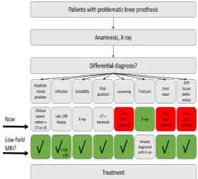
Figure 7: Overview of the methods available for the diagnosis of problematic total knee prosthesis pathologies (from MRIPro voucher request).

Magnetic resonance imaging (MRI) has the ability to image all tissues of the body and low-field MRI is expected to reduce the metal artifacts in MRI data. Therefore, low-field MRI may provide an alternative imaging method for the simultaneous diagnosis of problematic TKA pathologies, and liner wear and malalignment in particular.

The main research question for this study is: Can low-field MRI provide an alternative for the current clinical practice, for the simultaneous diagnosis of malalignment and liner wear for prob-lematic total knee prosthesis patients?

This research question will be divided into the following sub-questions:

Can low-field MRI determine prosthesis component malalignment of the problematic total knee prosthesis?

Can low-field MRI determine the polyethylene liner wear of the problematic total knee prosthesis?

3.4

Study Design

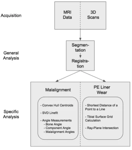
Figure 8: Flowchart of the study.

4

Theory

In this section, the imaging modalities used for the diagnosis of various pathologies of the prob-lematic total knee prosthesis are presented.

4.1

Common Orthopaedic Imaging

Various imaging modalities are used for the diagnosis of problematic total knee arthroplasty (TKA) pathologies. X-ray, ultrasound(US), computed tomography(CT), r¨ontgen stereophotogrammetric analysis (RSA), and magnetic resonance imaging (MRI) can be employed to determine different underlying pathologies of TKA problems. Each imaging method provides advantages and disad-vantages, described here and shown in the overview (table 1) at the end of this section.

X-ray imaging of the knee is routinely used for the assessment of the components of the total knee prosthesis. Some strong advantages for x-ray imaging is that it does not suffer from pro-nounced metal artifacts, is fast, and is widely used in orthopaedics, and clinical and research settings. The major disadvantage of X-ray imaging is that it is a 2D imaging method and it is difficult to correctly position the region of interest to obtain an ideal image for objective measure-ments. Also, performing an X-ray exposes the patient to radiation, which is ideally avoided. [52]

Ultrasound (US) imaging in orthopaedics can be used for the assessment of the prosthesis liner. However, the penetration depth is very low, due to scatter and absorption of the ultrasound waves by various tissues, especially dense tissues. Therefore, US is not very useful for the imaging of structures deep in the knee.

Computed tomography (CT) is a fast and accessible imaging technique for the imaging of the musculoskeletal system, among others. CT is also a R¨ontgen based technique, however, in contrast to the x-ray, CT is a 3D imaging method. A major disadvantage of CT, and R¨ontgen imaging methods in general is that it has low soft tissue contrast. Furthermore, metal artifacts are present

e.g. in the form of streak artifacts near and between metallic objects in the imaged volume. [53]

R¨ontgen stereophotogrammetric analysis (RSA), is an analytical imaging method specifically used for the measurement of prosthetic migration. This method is very accurate and is often used for the measurement of micro-motion to predict and monitor aseptic prosthesis loosening. The major disadvantage of this method is the requirement of per-operatively placing peri-prosthetic tantalum markers, which makes this analysis method available in a research setting only. [54–58].

4.2

MRI

Magnetic resonance imaging (MRI) is an imaging technique widely used in clinical practice. It can image all of the various tissues in the body, making it very suitable for the imaging and diagnosis of musculoskeletal pathologies [59]. The following section provides background information about the MRI technique and an introduction to low-field MRI.

Many molecules in the body have magnetic properties, however, for standard MR imaging, the magnetic properties of bound hydrogen (1_{H) nuclei are used to obtain images. Each hydrogen}

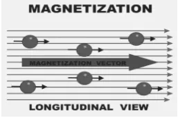
Figure 9: The figure above shows the direction of the magnetization vector, parallel to the main magnetic field lines from theB0 field. [61]

WhileM is a three-dimensional vector consisting of x-, y-, and z-directional components, when a homogeneous external magnetic field is present, the x-, and y-components are 0 and only its z-component is present and at its maximum,Mz=M0. After excitation by a radio-frequency (RF)

pulse the x-, and y-components of Mbecome larger. During an MRI scan,Mis excited by an RF pulse, causing it to rotate away from its original orientation,Mz, by an angleα, known as the flip

angle, toMxy. The initially coherent spins of Mwill then start to rotate or precess aroundB0 by

angleαand with frequency:

flarmor =γB0 (1)

whereγis the gyromagnetic ratio of a proton, which is equal to γ= 42.58M Hz/T.

4.2.1 Susceptibility Artifacts

For many MRI applications, it is crucial to supply spatial information of the volume. To provide this spatial encoding, gradients are used. When applying a gradient to the B0 field, the field

strength increases fromB0−zGz to B0+zGz, with Gz the change in field strength per unit of

length (e.g. 1mT/cm), z the distance from the center of the gradient. In MRI, an individual slice can be excited by an RF-pulse that corresponds to the specific resonance frequency of the protons in that slice:

f =γ(B0±zGz) (2)

However, the presence of metallic objects can cause problems with this method, due to the intrinsic properties of metallic objects and MRI itself.

When metals are placed in a magnetic field, in this case the homogeneousB0 field, they induce

an internal magnetic field that disturbs theB0field lines. This causes a change in the strength of

the magnetic field around the metal and consequently alters the resonance frequency of the spins in that area. The corresponding resonance frequency of the affected spins becomes

f =γ(B0+Blocal) (3)

which differs from the original larmor frequency from equation 1. The spins around a metallic object are subject to both the field gradient (B0 and the magnetic field distortion (Blocal) of the

Figure 10: Effect of metal objects on the spatial encoding of a volume. The excitation profiles show the positions of the excited spins for the resonance frequency of several slices resulting from a scan with a metallic ball, viewed from above. Due to susceptibility, the white bands representing the excited spins, are not a straight line, which is expected when exciting a single slice. Furthermore, other spins not expected in the slice are also excited. [62]

The strength of the magnetic susceptibility artifact caused by the presence of a metallic object is proportional to the strength of the main magnetic field by the relation:

∆r∝k∆χB0

G (4)

where ∆r is the pixel shift in the imaging plane, k is some proportionality constant depending on the shape of the object, ∆χ is the difference in susceptibility between the material and the surrounding tissue, B0 is the strength of the main magnetic field, and G is the strength of the

readout gradient [63].

4.2.2 T2 Relaxation

Apart from the above relation between metallic objects and a magnetic field, another mechanism causes artifacts due to the presence of metallic objects. This mechanism is embedded in the relaxation parameter T2, that determines much of the signal measured with MRI.

It has previously been stated that an RF-pulse rotatesMand causes it to precess aroundB0with

resonance frequencyf. To detect a signal from this precession we must turn to Faraday’s law of induction which states that a change in magnetic flux generates an equally large, but oppositely charged electromagnetic force in a nearby conductor:

ε=−δφB

δt (5)

whereεis electromagnetic force,φB is magnetic flux, andt is time. The measurable precession of

MaroundB0, however, does not maintain its strength infinitely due toMreturning to its original

alignment along the B0 field lines. This process is called relaxation and is determined by two

parameters, T1 and T2, and results in a free induction decay (FID) signal. The relation between magnetization, T1 and T2 is given by:

Mxy=M e−t/T2 (6)

Mz=M0(1−e−t/T1) (7)

caused by molecular interactions and are random by nature due toe.g.Brownian motion, electron shielding, and other mechanisms [64]. The resulting magnetic field inhomogeneities are very small, yet cause the individual spins ofMxy to lose phase coherence and therefore causes T2 relaxation.

During an MRI scan, however, signal decay is normally much faster than the expected T2 would predict. This is due to field inhomogeneities on a larger scale. The presence of an object, such as a hand, in the scanner, will disturb the main magnetic field, causing changes in local magnetic field strengthBlocal. This type of T2 relaxation is called T2*-relaxation and is defined as:

1

T2∗ = 1

T2+γ(B0±Blocal) (8) While T2 relaxation based on the molecular interactions is random and cannot be corrected, these larger local changes are static and can be corrected. This is done by introducing a 180°RF-pulse, which flips the spins and the phase differences. The flipping of the spins and phase differences causes the spins to re-phase and create an echo. This echo is the signal that would be measured if only T2 relaxation was present. Figure 11 illustrates this principle, where the red arrow represents the magnetization vectorM.

Figure 11: The illustration above shows the principle of a Spin Echo (SE). After a 90 degree RF-pulse,Mrotates and its spins start to de-phase. After a subsequent 180 degree RF-pulse, the spins re-phase and create an echo.(from [65])

When considering the disturbances of the B0 field by a metallic object, the difference of the

susceptibility between the metallic object and the surrounding tissue must be taken into account. From Schenket al. [66] it can be seen that this difference is up to 103 _{larger than the differences}

between water based tissues in the body. As such, the metallic objects in standard clinical 1.5T MRI have a large effect on the T2* relaxation of the signal as well as the spatial encoding of the volume. To provide lower metallic artifacts in the image data, low-field MRI was used in this study. Below, further information on low-field MRI is provided.

4.3

Low-field MRI

Standard clinical MRI scanners work with main magnetic fields in the range of 1.5−3.0 tesla [64]. Low-field MRI is defined as having a main magnetic field below 0.3 tesla. To see what a lower magnetic field does to the strength of the signal, the Boltzmann equation can provide some insight [60]:

M0=B0

γ2h2Ns

4kT (9)

When disregarding the other terms, we can instantly see that M0 ∝ B0. For a 0.25T scanner,

such as the one considered in this study, the expected M0 will be at least six times smaller than

arthroscopic findings [68].

One resulting advantage of the lower magnetic field strength of low-field MRI is its effect on susceptibility artifacts. From the relation between the strength of susceptibility artifacts and main magnetic field strength in equation 7, we can also derive that the strength of the artifact in low-field MRI should be lower than that of standard MRI. Indeed, Farahaniet al.(1990) [69] have also shown this is the case.

Furthermore, one of the main advantages of the low-field MRI present at the University of Twente is the availability of weight-bearing scanning. The clinical imaging for malalignment and liner wear is performed in standing position. Low-field MRI can mimic the standard radiology exams for total knee prosthesis imaging as described in literature [31, 46].

Beyond the advantage of lower strength susceptibility artifacts, low-field MRI can have several other advantages depending on specific designs:

• Open design

• Cheaper

• Lower energy deposition in tissues

4.4

Overview

In the paragraphs above, a theoretical background is provided to show how low-field MRI may affect MR image data. While MRI can image all tissues In the paragraphs above, an intuition of how MRI and specifically low-field MRI can aid the analysis ofin vivoprimary total knee prosthesis is presented. Furthermore, several other available diagnostic imaging methods have been discussed. Here, an overview of the advantages and disadvantages of the available imaging methods is given.

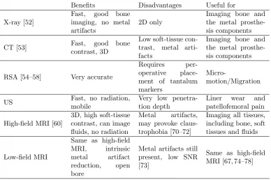
Table 1: A summary of the advantages and disadvantages of CT, X-ray, high-field MRI and low-field MRI for imaging TKPin vivo.

Benefits Disadvantages Useful for

X-ray [52]

Fast, good bone imaging, no metal artifacts

2D only

Imaging bone and the metal prosthe-sis components

CT [53] Fast, good bone

contrast, 3D

Low soft-tissue con-trast, metal arti-facts

Imaging bone and the metal prosthe-sis components

RSA [54–58] Very accurate

Requires per-operative place-ment of tantalum markers

Micro-motion/Migration

US Fast, no radiation,

mobile

Very low penetra-tion depth

Liner wear and patellofemoral pain

High-field MRI [60]

3D, high soft-tissue contrast, can image fluids, no radiation

Metal artifacts, may provoke claus-trophobia [70–72]

Imaging all tissues, including bone, soft tissues and fluids

Low-field MRI

Same as high-field MRI, intrinsic metal artifact reduction, open bore

Metal artifacts still present, low SNR [73]

5

Data Acquisition and General Analysis

This section will describe the materials and methods and results for the Data Acquisition and General Analysis parts of the study as well as provide a section specific discussion. The data acquisition and general analysis consist of the MRI data acquisition, the acquisition of the 3D optical scans, the segmentation and registration segments of this study.

5.1

Materials and Methods

5.1.1 MRI Data Acquisition

Primary Dataset

A primary dataset of a scanned patient with a primary total knee prosthesis was available and used as a template to determine the intra-observer variability of the image segmentation and to de-velop the malalignment and liner wear workflow and measurements. This dataset was not created following the protocol described below but was previously available as a sample for the purpose of development. This data is denoted as Pt. 101.

Patients

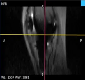
For this study, data was obtained from patients all under care at OCON Hengelo who have given informed consent for the use of their low-field MRI data to be used for this study. One patient with and six without residual pain are included. Excluded are patients with a contra-lateral TKP, an inability to stand for 15 minutes, or a contra-indication for undergoing an MRI scan. The included patients are scanned at the University of Twente at the Esaote low-field (0.25T) scanner (Esaote G-scan brio, Esaote SpA ©2017, fig12). Scans are made with knee coil 1 with the patient in a vertical position (81.0° angle). This is done to mimic the current clinical practice for radiology examination of the knee, which is a standing, load-bearing radiograph. Furthermore, patients are scanned in supine position as well. For comparison, one of the patients’ supine data set is used for analysis. Patients are numbered 102-107a for the patients without complaints of the knee, 201 for the patient with complaints of the knee, and 107b for the patient data acquired in supine position.

Figure 12: Low-field MRI scanner at the University of Twente (Esaote G-scan brio, Esaote SpA

©2017). Shown orientation not known, however, the figure illustrates the possibility of different angles of the scanner to allow for weight-bearing positions. (From Esaote documentation [79]

MRI Scan Protocol

Images were acquired using a T1 spin-echo sequence. Sagittal images of the data were used for further analysis with dimensions: 256×256 voxels per slice, 0.89×0.89mm2_{pixel size and a pixel}

(a) Transverse plane in the planning stage of the low-field MRI scanner. The pink line represents the global x-axis and the blue line representes the global y-axis.

(b) Sagittal plane in the planning stage of the low-field MRI scanner. The pink line represents the global z-axis and the yellow line represents the global y-axis.

Figure 13: Alignment phase of the planning of an MRI scan.

5.1.2 3D Scans

Optical Scanning of Components

3-Dimensional models of the tibial and fibular components of the total knee prosthesis have been made with an optical 3D scanner at the University of Twente (Konica Minolta Vivid 910) and processed in Meshmixer 3.3 (©2017 Autodesk, Inc.). The total knee prosthesis components that were scanned and used for this study are the Smith and Nephew GENESIS II components. The scanned models were femur size E right and tibia size 5. Because only one set of components was available for the optical scan, the obtained femoral and tibial component scans were linearly scaled to also estimate models of the other possible sizes, using the values given in [80]. During the processing step, the prosthesis components (both femoral and tibial) are aligned with the global coordinate system as defined in the MRI data acquisition section. The resulting models are used during the registration step.

(a) Example of a femoral component of a TKP.

(b) Example of a tibial component of a TKP

Figure 14: 3-Dimensional models of the tibia and femur components of the total knee prosthesis obtained from the 3D optical scanner.

3D Model Alignment

Resulting from this alignment are femoral and tibial components in the ideal alignment. This alignment of the 3D models results in a separate set of components for each component and liner size combination. Alignment of the components was performed in Meshmixer and 3-Matic. This alignment and positioning is performed in order for the registration to work correctly. The 3D model and the segmented data must be in each others proximity, and, ideally, aligned similarly, which is achieved in this step. If the segmented data and the 3D models are not near each other when loaded into Mimics, the registration algorithm fails.

5.1.3 Segmentation

After data acquisition, but prior to image analysis or measurements, image segmentation must be performed. It is a crucial step towards further image analysis, however a difficult task due to the metal artifacts present in the MRI data. While many (semi-)automatic segmentation algorithms exist, manual segmentation remains the gold standard for image segmentation [81, 82]. There-fore, manual image segmentation will be performed to obtain segmentation models of the relevant structures from the MRI data. Segmentation will be performed in Mimics Innovation Suite 19 ( Copyright Materialise 2017). During the segmentation step, the tibia, femur, tibial prosthesis component, and femoral prosthesis component are segmented. The resulting segmentations will be rendered as 3-dimensional models to be used for later registration and analysis.

To determine the variability of manual segmentation with Mimics for segmenting the femur, tibia, femoral prosthesis component, and tibial prosthesis component, three separate segmentations were performed and analyzed. The intra-observer variability was determined by calculating the DICE and Jaccard similarity coefficients. This provides segmentation similarity measures for the manual segmentation of the femur, tibia, femoral prosthesis component and tibial prosthesis component in low-field MRI data sets with a total knee prosthesis.

The DICE score is determined by the pixels present in both segmentations (|A∩B|) and the pixels in each segmentation (|A|and|B|). The DICE coefficient is calculated as follows:

DICE= 2|A∩B|

|A|+|B| (10)

From this, the Jaccard score can be calculated as:

J accard=DICE/(2−DICE) (11)

While both the DICE and Jaccard coefficients describe the similarity of two segmentations based on the overlap of voxels in the segmentations, the main difference between the DICE and the Jaccard scores is the rate at which they grow. The DICE score will become larger faster than the Jaccard. which may provide more promising results than may actually be the case. A DICE or Jaccard alone does not say too much about the agreement between the datasets, while examining both simultaneously provides more insight in he similarity of the segmentation results.

5.1.4 Registration

5.2

Results

5.2.1 Patients

All patients in this study gave informed consent for the use of their low-field MRI data for this study. Included were seven patients without symptomatic total knee prosthesis and one with symp-tomatic total knee prosthesis. Age, sex and prosthesis age are shown in table 2. Prosthesis age is time between the date of the TKA procedure and the date of scanning the patient with the low-field MRI scanner. The average age of the patients included in this study is 67 years. There are 4 women and 3 men in the non-symptomatic total knee prosthesis group, with an average prosthesis age of 493 days. The patient with symptomatic total knee prosthesis, however, has a prosthesis age of more than 9 years.

Patient Age(years) Sex Prosthesis Age(days)

101 62 F Unknown

102 62 M 374

103 66 M 422

104 58 M 497

105 78 F 637

106 61 F 454

107 78 F 573

201 67 F 3387

Table 2: The age, sex and prosthesis age for the patients included in this study. Note the large difference in prosthesis age for patient 201(with symptomatic knee prosthesis) compared with the other patients).

The femoral component, tibial component and PE liner sizes of each individual patient is shown in table 3. This information is crucial for the registration step, as well as for the interpretation of the liner wear results. As can be seen from the table, the femoral components range from E to F, whereas the tibial component size range is from 3 to 7. The liner size is the same for all patients except patient 104.

Patient Number Femoral Component Size Tibial Component Size Liner Size (mm)

Pt 101 E-R 3 10

Pt 102 G-L 6 10

Pt 103 F-R 5 14

Pt 104 G-L 7 10

Pt 105 F-R 4 10

Pt 106 E-R 3 10

Pt 107a E-R 6 10

Pt. 201 F-R 4 10

Pt. 107b E-R 6 10

Table 3: Size of the knee prosthesis components for the patients included in this study. Femur size is denoted as the component size followed by an L or R for left or right. This data is important for the registration step, as it is of crucial importance to register the correctly sized 3D models to the segmentation. Also, it provides insight in the liner wear measurements. The pre-registration models that are used for the ideally aligned measurement are of sizes: Femur E-R, Tibia 5, Liner 10.

(a) (b) (c)

Figure 15: Several of the images retrieved from the low-field MRI scans performed on the patients. These images present a few of the major difficulties of imaging a total knee prosthesis with low-field MRI. a) shows a very short femur (red arrow), b) shows a movement artifact(blue arrows), and c) presents an example of the artifacts present in each data set(green arrowheads) as well as a wraparound artifact (white arrowhead). While these artifacts are also present in standard clinical MRI, the artifacts in the low-field MRI data was not expected to be this large.

5.2.3 Segmentation

(a) (b)

(c) (d)

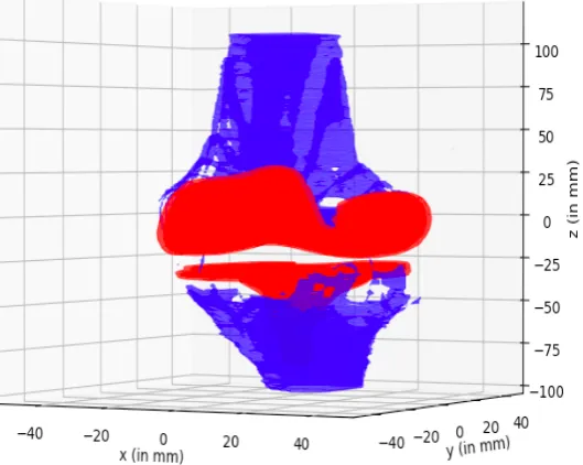
Figure 17: A complete segmentation of a single MRI dataset. All relevant bony and prosthesis structures have been segmented: femur and tibia (blue), and the femoral and tibial components (red).

Seg1 v Seg2 Seg1 v Seg3 Seg2 v Seg3

Complete segmentation

DICE 0.63 0.57 0.76

Jaccard 0.46 0.40 0.61

Bone Segmentations

Femur

DICE 0.67 0.66 0.72

Jaccard 0.51 0.49 0.56

Tibia

DICE 0.61 0.63 0.73

Jaccard 0.44 0.46 0.57

Component Segmentations

Femur

DICE 0.80 0.80 0.87

Jaccard 0.67 0.67 0.76

Tibia

DICE 0.69 0.79 0.80

Jaccard 0.53 0.65 0.67

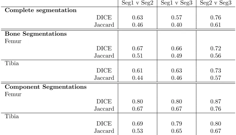
Table 4: DICE and Jaccard scores of the three manual segmentations made with the primary low-field MRI dataset. A higher value indicates a better agreement between datasets. The component segmentations show a higher agreement between segmentations than the bone segmentations for all three segmentations. Seg1 is the first segmentation, Seg2 the second, and Seg3 the third segmentation.

5.2.4 Registration

Table 5 shows the results of the registration algorithm applied in Mimics to register the 3D models from the optical scanner to the segmentation models obtained from the previous segmentation step. The numbers presented are the remaining least squares error distance inmm, and a higher error indicates a less accurate registration, where the most accurate registration provides no remaining error.

Femoral Component Registration (mm) Tibial Component Registration (mm)

Pt 101 1.7127 2.3497

Pt 102 2.0617 2.3634

Pt 103 2.6073 2.5391

Pt 104 2.1047 1.8896

Pt 105 2.5613 2.5110

Pt 106 2.6772 2.2738

Pt 107a 2.0715 2.5625

Pt 201 2.3090 2.3224

Pt 107b 2.6361 2.1214

5.3

Discussion

5.3.1 MRI Data Acquisition

As the results in figure 15 of the MRI data acquisition show, the data contains many artifacts. It was hypothesized that the use of low-field MRI would diminish the susceptibility artifacts caused by the presence of metals, such as that the shape of the metallic prosthesis components would be better visible than with a standard MRI exam. However, as can be seen from figure 15c, the susceptibility artifacts are still present, and it remains difficult to distinguish the individual components and identify the correct shape of the components. Standard MRI of a total knee prosthesis also shows significant artifacts (figure 18). The images from this study show similar artifacts shown in figure 10, indicating that the image quality with respect to metal artifacts of low-field MRI is not as good as expected.

Figure 18: Sagittal MR images of a TKR in a healthy volunteer. Metal-induced artifact including distortion (wedge-shaped arrow) and signal loss (curved arrow) severely limit the diagnostic value of Fast Spin Echo (FSE) images. (image from Chenet al. [83])

Furthermore, the pixel spacing, or slice thickness, of 4.4mm between slices is very large, which increases the strength of the partial volume effect when compared to smaller voxels. This may be of importance when considering susceptibility artifacts. A smaller slice thickness means that the artifact does not provide as much of a pixel shift (∆r in equation 7) in the image. Therefore, decreasing the pixel spacing between slices, may provide more spatial resolution and could possibly decrease the size and intensity of the susceptibility artifacts present in the current images. The use of promising magnetic artifact reduction sequences such as MAVRIC and SEMAC-VAT [84, 85], has been shown decrease metal induced susceptibility artifacts and increase the image quality. In this study, these sequences were not used as these specific sequences are not available on the low-field MRI at the University of Twente. Other sequences are available, such as X-MAR sequences, however, during the selection of the sequences that will be used for the imaging protocol, the X-MAR sequences were deemed of low quality compared to the images used currently. Considering the extent of the susceptibility artifacts in the data, the current images do not provide the artifact reduction that was expected from using low-field MRI. As such, a more artifact reducing sequence should be considered in the future if low-field MRI is to be used.

5.3.2 3D Scans

3D optical scans were obtained with an optical scanner at the University of Twente. These models are representations of the real-world prosthesis components. The component scans contain upwards of 15000 faces for a femoral or tibial component scan. After reduction of the faces, upwards of 7500 faces are still present. This is extremely large and partly causes the malalignment and liner wear measurements in which these models are used, to be fairly slow (several hours for 15000 faces, 45 minutes for 7500 faces).

As described in the above methods section, only one size of each prosthesis component was scanned, while the other size models were scaled from the scanned data. This does provide the correct medio-lateral and antero-posterior dimension, however, the scaling is uniform. The actual prosthesis components are not uniformly scaled from one size to another [86].

in the clinical practice of OCON. Ideally, the CAD-models from the manufacturer would provide more accurate registration results and possibly provide more accurate liner wear and malalignment results as well.

5.3.3 Segmentation

For the data in this study, a high score of 0.76 and 0.61 in the DICE and Jaccard scores, re-spectively, were found for the similarity of the complete segmentation of segmentation 2 and 3. These scores can be attributed to the lower scores found for the bone segmentation than for the component segmentation. As table 4 shows, the bone segmentations for both the tibia and the femur have a lower similarity than the component segmentations for all of the segmentations. This indicates that the bone is more difficult to segment than the component, while this would not necessarily be expected, given the presence of artifacts at the expected position of the components in the images.

The average similarity of the segmentations falls below the 0.70 threshold, above which is con-sidered good agreement [87], for both the DICE and Jaccard scores, indicating the segmentation method is not very reproducible. This finding further supports studies showing manual segmenta-tion has a high intra-observer variability [81, 82].

While manual segmentation remains the gold standard for segmentation methods [81, 82], studies have shown that the intra-observer variability is significantly lower for semi-automatic segmenta-tion than for manual segmentasegmenta-tion of distinct structures [88, 89]. Due to the remaining presence of artifacts in the low-field MRI data, accurate (semi-)automatic segmentation of the prosthesis components is difficult. The absence of defined contours of the prosthesis components and the bone segments, makes automatic algorithms based on thresholding or shape matching difficult to implement. As such, manual segmentation was performed for the segmentation task in this study. The use of (semi-)automatic segmentation may provide faster and more robust segmentation of the data, however image quality must improve. Metal artifact reduction sequences have shown to improve image quality of MRI exams of metallic objects [84, 85, 90]. Applying these sequences may provide a basis for the application of (semi-)automatic segmentation algorithms.

The segmentation results also show higher similarity coefficients of the component segmentations. This implies that the segmentation of the components in not necessarily the biggest issue with the method, whereas that was initially expected. The component segmentations even reach a good agreement or better (above the 0.70 threshold) for both the DICE and Jaccard coefficients for both the femoral and tibial component segmentations.

Other similarity coefficients, such as the Hausdorff distance were also considered, however, they were not expected to provide interesting information in addition to the DICE and Jaccard coeffi-cients. The Hausdorff distance measure determines the closest distance of erroneous segmentation voxels from the ground truth segmentation. Here, a manual segmentation method was applied where singular outlying voxels can easily be spotted and removed from the segmentation during the manual segmentation step in Mimics. The Hausdorff distance was therefore not considered to provide interesting information about the similarity of the segmentations. [91]

5.3.4 Registration

6

Specific Analysis: Malalignment

This section will describe the materials and methods and results for the malalignment part of this study, as well as provide a measurement specific discussion of the method and results. The malalignment measurement is part of the specific analysis segment of this study.

6.1

Materials and Methods

Malalignment is measured in several steps. First, the anatomical axis or mid-shaft line of the bone is determined using a convex hull measurement. Then, the corresponding axis of the registered prosthesis is calculated. Lastly, the angle between the two axes is determined, which provides the relevant angles to determine the cFA, cTA, sFA, sTA, and TFA. The method described below is performed for both the femur and the tibia, for sagittal and coronal orientations.

Convex Hull Centroids

To determine the relevant angles as shown in figure 5, the anatomical axis of the bone should be calculated. To provide the anatomical axis, a similar approach to Stanet al.(2013) [39] and Mirandaet al.(2010) [92] is taken, where the convex hull is used to calculate the central points of the bone and a line through the central points is determined. The convex hull is an algorithm to determine the smallest convex set of points that contains all the points in the respective slice. An analogy is shown in figure 19, where an ”elastic band” is stretched around a set of nails/points. Then the band is let loose, the form and position of which then represents the convex hull of the set of points.

Figure 19: Example of the convex hull calculation. Here, the wide circle represents the stretched elastic band and the dotted line represents the resulting convex hull when the band is released. The points are random points in 2D space. (From [93])

After the convex hull is determined, the respective surface area and centroids can be calculated. The surface area is an important parameter to determine which slices will be taken into account for further analysis. The centroids of the convex hull surfaces combine to create the set of centroids that will be used to approximate the anatomical axis of the bone.

Convex Hull Surface Area

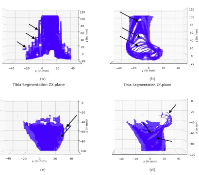
(a) Surface area of the convex hulls calculated along the femur.

(b) Surface area of the convex hulls calculated along the tibia.

Figure 20: Convex hull surface area for each slice along the z-axis of the segmentation. Furthermore, the black line shows the slices that are taken into account for determining the mid-shaft of the bone,i.e. up to 1/4th _{of the maximum convex hull surface area.}

This is done to account for outliers that can occur due to segmentation issues. Furthermore, dur-ing TKA surgery, a large part of the femur is removed, rejectdur-ing the assumption in Miranda et al.(2010) [92] that the distal part of the femur has the largest surface area by default. Hence, all data above 1/4th_{of the maximum convex hull surface area is used for further analysis and}

measure-ments. Examples are shown in figure 16, where the blue mesh represents the bone segmentation.

Centroid Calculation

The convex hull centroid coordinates Cx and Cy are calculated by [95]: Cx = 61A N−1

P

i=0

(xi + xi+1)(xiyi+1−xi+1yi)

Cy =₆1_A

N−1

P

i=0

(yi+yi+1)(xiyi+1−xi+1yi) where A is the convex hull surface area, N is the amount of

vertices contributing to the convex hull andxiandyi are thexandycoordinates of theithvertex

of the convex hull. The z-coordinate of the convex hull centroid corresponds to the z-coordinate of the slice for which the convex hull is calculated. The collection of centroids is used for further analysis and approximation of the anatomical axis of the bone.

SVD Line fit

Figure 22: Corrected set of centroids of the z-slices of the femur and tibia segmentation in the coronal and sagittal planes. The line in each figure is the SVD fit of the data. The upper two images are femoral and the lower two are tibial centroid data fits. As can be seen, the outliers highlighted in the previous uncorrected data are no longer present.

Angle Measurements

The angles that are calculated as described below, are calculated with respect to the unit circle shown here. A negative angle, therefore, means that the angle between the calculated axis and the global Z-axis is in a clockwise direction. As such, an angle in counterclockwise direction is a positive angle.

Figure 23: Unit circle indicating the direction of a positive angle [96].

(a) (b)

Figure 24: Results of the angle calculation of a testing cylinder when varying the convex hull surface area cutoff value. The cylinder was placed at a set angle (blue) in the ZX-plane, then the central axis was determined and the angle in the ZX-plane was calculated (red).

Due to the MRI scanning method, it is not expected that the angles measured in this study will not be very large, therefore, a more accurate measurement for the lower angles is important. As such, the 1/4thconvex hull surface area cutoff value is used for the analysis.

Bone Angle

The angles of the bone with respect to the global z-axis are calculated by determining the pro-jection of the line provided by the SVD linefit on the zx- and zy-planes. From here, the inherent calculation using the dot product results in the angle between two lines:

θ=|A||B|cos−1 (12) where A is the projection of the linefit on the plane, B is the global z-axis and Φ is the angle between A and B in radians. The angles that are calculated for the sagittal and coronal planes are

θsagboneandθcorbone respectively.

Component Angle

The prosthesis component is aligned to the global coordinate system, as described previously in the methods section,i.e. the x-, y-, and z-axes of the prosthesis component LCS are the same as the GCS. During the registration step, the prosthesis component is registered to the 3D segmentation in Mimics Innovation Suite 19. This provides a 4x4 registration matrixT, that includes a transla-tion (t) and a rotatransla-tion (R). The registered prosthesis component axes are calculated by applying the registration matrix Tobtained in the registration step, to the GCS. In a similar manner as above, the angles between the z-axis of the registered prosthesis component and the x- and y- axes of the GCS (θcorprotandθsagprot, respectively) are calculated.

Malalignment Angles

Figure 25: The angles cFA, sFA, cTA and sTA will be calculated as shown in the above image. Here, the sFA parameter has a positive angle. In this figure, the CBA and TFA are not shown. (Image adjusted from [38]

Expected Results

From Stan et al. [39], the recommendation is to balance the components to minimize the forces on the tibial plate and tibia. A component balance angle (CBA) of 180°is recommended by Stan

6.2

Results

For the malalignment measurement, a line was required to be fit to the centroid data. In this study, an SVD linefit was used for determining the straight line through the centroids. A least squares algorithm was also considered, however, it was deemed that the resulting line did not match the data as well as the SVD line fit did considering the results shown in figure 26. From these figures it was considered that the SVD line fit performed superior to the least squares algorithm and was therefore used for the calculation.

Figure 26: The above figures show the line fits of femoral centroids made with the SVD and least squares methods. As can be seen, the SVD fits the data better than the least squares estimation.

The results of the malalignment measurement for each dataset are given in table 6. Figure 27 provides a reference for the calculated angles.

Figure 27: Malalignment angles calculated in the malalignment measurement. The cFA, cTA, sFA and sTA are shown in this image. It should be noted, in this figure, the sFA parameter is positive. The TFA is not shown but is calculated as the angle between the tibial and femoral anatomical axes. Furthermore, the CBA is also not shown here, however is simply calculated as: cF A+cT A. (Image adjusted from [98])

cFA(°) cTA(°) sFA(°) sTA(°) CBA(°) TFA(°)

Clinical Range 84-94 87 0 90 176 177-187

Pt. 101 88.41 101.63 -5.32 84.69 190.04 176.29

Pt. 102 87.56 101.96 -12.77 92.21 189.52 180.09

Pt. 103 88.78 96.39 -7.60 80.59 174.83 176.82

Pt. 104 94.50 91.67 -2.66 92.96 186.17 192.19

Pt. 105 94.21 87.66 -5.65 87.15 178.13 167.11

Pt. 106 89.72 97.41 -12.87 87.80 172.87 179.96

Pt. 107a 93.35 90.81 3.11 89.16 175.84 174.21

Pt. 201 83.64 99.17 -7.50 88.93 177.19 183.26

Pt. 107b 103.04 83.31 -0.08 84.02 173.65 156.01

Table 6: Calculated values of the malalignment angles. cFA = coronal femoral angle, cTA = coronal tibial angle, sFA = sagittal femoral angle, sTA = sagittal tibial angle, TFA = tibiofemoral angle, CBA = component balance angle. The bold values are within the clinical reference range (or within 5 degrees of a single clinical reference value).

The figure28 shows the boxplots of the healthy patient data with the scanner in vertical (standing) position (Pt. 101-107a). It should be noted that the whiskers of the boxplot reach to 5% and 95% of the dataset, whereas the boundaries of the box are the second and third quartile of the data. Also, the clinically expected values for the cFA, sFA, TFA and CBA (green values in the plot) fall (at least partly), within the 95% CI range of the data. For the cTA and sTA, the reference values fall outside of the 95%CI of the values found in this study.

Figure 29: Boxplots with 95% CI of the malalignment angles calculated in the malalignment measurement. The red data indicates the values found for the patient with symptomatic total knee prosthesis.

Figure 30: Boxplots with 95% CI of the malalignment angles calculated in the malalignment measurement. The blue data indicates the values found for the data scanned with the patient in supine position (scanner in horizontal position).

The figures (29 and 30) show the results of the measurements made with the scanner in horizontal position (30), and with a patient with symptomatic total knee prosthesis(29). Figure 29 shows that the values calculated for the patient with symptomatic total knee prosthesis are within the 95% CI ranges of the sFA, sTA, TFA and CBA found in this study. For the cFA and cTA the values calculated for the symptomatic patient fall outside of the 95%CI range as well as the clinical reference value ranges. It should be noted however, that except for the cFA, the results for the symptomatic total knee prosthesis patient are within the ranges of the healthy controls.

6.3

Discussion

As indicated earlier, the cTA and sTA angles are higher and lower, respectively, than the values that have been indicated in literature [99]. However, other research shows directly post-operative angles of 87 and 84 for cTA and sTA, respectively [98], which more closely resemble the values found in this study. Furthermore, Kilincogluet al. also reported sFA values of 6.6±2.4, whereas other studies do not disclose or determine these values. These reported values are measured di-rectly post-operatively, whereas in this study the average age of the prosthesis components is 493 days. A reason for the differences in values may be due to possible micro-motion that takes place over time.

The differences in the values found with the method presented in this study compared to the clin-ical reference values, imply that the method is currently not accurate enough to provide reliable measurements for clinical application. As stated above however, the differences in these values may be due to the prosthesis age of the patients in this study, which may explain the large variance in the results shown in figure 28. However, from the same figure, as well as table 6 it can also be seen that a large part of the values do correspond with the clincally relevant reference values. This implies that the method does have the capacity to determine the malalignment values for the clinical ranges. As such the method does show promise for future applications.

Another finding is that the results of the patient with remaining complaints of the total knee prosthesis, pt. 201, are not very different from the other results. When inspecting the results, it can be seen that the results for pt. 201 only differ from the non-symptomatic total knee prosthe-sis patients results in the calculated cFA. This lack of dissimilarity between the results may be caused by the inaccuracies of the segmentation that subsequently influence the registration and the malalignment measurement. However, it could also be that the pathology of the patient is not caused by the malalignment of the prosthesis components and complaints originate from other pathology.

Lastly, it is interesting to note that the femoral measurement for pt. 102, does not differ in the coronal direction but does in the sagittal direction. Due to the short femur in the image data of pt. 102, the malalignment measurement for the femoral variables is expected to possibly differ from the other measurements in the study. However, this does not seem to be the case for the coronal femoral angle. As such, it seems that the measurement is robust in the coronal plane. This may imply that the minimum length of the femur required in the image for adequate anatomical axis approximation may not be 5.5mm as suggested by Mirandaet al.(2010) [92] for the coronal plane.

For the malalignment measurement, only the data of slices with a convex hull surface area of more than 1/4th _{of the maximum convex hull surface area were taken into account for further}

7

Specific Analysis: Liner Wear

This section will describe the materials and methods and results for the liner wear part of this study, as well as provide a measurement specific discussion of the method and results. The liner wear measurement is part of the specific analysis segment of this study.

7.1

Materials and Methods

Tibial Surface Grid Calculation

To measure the thickness of the PE liner of the prosthesi, it is assumed the liner is the only thing between the prosthesis components [15, 100]. Thus, the distance between the tibial and femoral components is the thickness of the liner. To calculate the distance from the surface of the tibial component that surface must first be defined. The tibial component mesh is split in various bins of vertices by dividing the surface in 1mm slices. As the tibial component surface is a flat structure, it can be assumed that in the pre-registration step the slice containing the surface of the tibial component will have the most vertices. This slice then provides the z-component of the tibial component surface in GCS coordinates.

Figure 31: Several points of grid G. The distance between the points in each perpendicular direction is 2mm.

Figure 32: Calculation of gridG of the original tibial component. From the registration matrix the new position of the tibial component as well as the new position of the grid is determined, providing the new gridGr. The blue arrow indicates that the registration matrix is applied to the

green grid and red component.

Shortest Distance of Point to Line

The shortest distance between a point P and a line l1 is the perpendicular line l2 from point P

to line l1 (see figure 33). The points representing grid G, are the initial starting points of the

perpendicular line in figure 33. The orientation of G is such that the global z-axis is its normal,n. By providing, for each point on G, a second point along the global z-axis above G, a ray can be defined by:

ray=P0 +k·P1 (13)

where P0 is the starting point of the ray on grid G and

P1 =P0 +n (14)

withn the unit vector normal of grid G. To obtain the positions and orientations ofray on the registered tibial component, the registration matrix resulting from the registration step is applied to G, resulting inGr. From this multiplication with the registration matrix, theray vectors also

rotate and translate and remain perpendicular to the defined grid.

Figure 33: Example showing the concept of the perpendicular line from a point to a line. Here, three lines are drawn from point P to line L. The minimum distance from P to L is the perpendicular line (5). (from [101])

Line Plane Intersection

p3, each of which are 3-dimensional, and determining the output of the following equation

F acenormal=a2b3−a3b2−(a1b3−a3b1)a1b2−a2b1 (15)

where a = p2−p1 and b = p3−p1. To calculate the intersection of the line and the face, an arbitrary point on the face is used, in this case the center of the face. From here, to calculate the position of the intersection, the equationP0 +k∗v must be satisfied for the parameter k, a scalar number determining the length of the line. Calculating the parameter k is achieved by again applying the dot product

k=knumerator/kdenominator (16)

where knumerator= (p1−P0)·normal

kdenominator=v·normalEnteringkinto the ray equation: P0 +k∗vprovides the 3-dimensional

position of the intersection between the line and the face. The intersection calculation is performed for eachray vector on the gridGr and for each face separately. Performing this calculation will

result in the same amount of intersections for each ray as there are faces in the mesh. Many of these intersections, however, are not relevant, as they are not within the boundary of the mesh, which is determined by the faces of the mesh. To determine whether the intersection is on a face, the face boundaries are used to determine a valid intersection. If the intersection falls within the face boundaries, an intersection is deemed valid, otherwise it is not.

The results of the liner wear measurement are provided as a heatmap, where the measured length is set out against the position of the respective measurement. A higher measured length corresponds to a darker color, and a smaller distance corresponds to a lighter color (see figure 34).

Figure 34: Presentation method of the liner wear measurement. Here, the result of a testing data set is shown where the distance from a 40mm x 40mm grid to a spherical object 10mm above the grid was calculated.

The thickness of the liner at the articulating surface is shown in table 7 for the range of liner sizes available. This information is crucial for the analysis of the measurement results. The articulating surface is the surface between the tibial plate and the femoral condyle(s) and represents the expected lowest value of the measurement for patients without liner wear.

Liner Size (mm) 10 12 14 17 20 Art. Surface Thickness(mm) 6 8 10 14 16

1mm and 2mm measurements. The high increase in distance near the posterior edge of the mea-surement can be seen in both meamea-surements as well as the ’v’-shape at the anterior side, however, increasing the distance between the points further may remove these important details from the result. For this study, the 2mm distance between points will be used.

(a) (b)

Figure 35: Measurement result for patient 107a with 1mm distance between the points a), and the measurement results for patient 107a with 2mm distance between the points b).

(a)

7.2

Results

Liner Wear Measurement Results

The measurement of the liner wear is represented as a distance heatmap. The result shown in figure 37 is the result from a liner wear measurement with the tibial and femoral components ideally aligned, i.e. directly above each other and without flexion/extension and varus/valgus. Here a right femoral component of size E, tibial plate of size 5 and a liner of size 10mm (articulating surface 6mm) are used. The darker the color, the higher the distance from tibial component surface to the femoral component.

Mean(mm) SD(mm) Minimum(mm)

Ideal Alignment 11.31 5.18 4.28

Pt. 101 39.15 5.33 32.29

Pt. 102 9.80 4.34 3.45

Pt. 103 14.47 6.75 4.98

Pt. 104 8.21 4.73 0.58

Pt. 105 11.56 4.56 5.34

Pt. 106 11.20 4.05 5.33

Pt. 107a 14.28 4.42 7.92

Pt. 201 15.47 5.97 4.94

Pt. 107b 18.42 4.85 11.06

Table 8: Calculated mean, standard deviation and minimum values of the liner wear measurement for all patients in the study. All values are inmm. Note the very large mean and minimum of Pt. 101 compared to the other measurements.

Note that this initial measurement shows that the distance is expected to be lowest in the center, at the articulating surfaces, and highest near the anterior-posterior edges of the component (Ideal Alignment results in table 8). Furthermore, it must be noted that the measurement does not rep-resent the shape of the liner. The actual shape of the liner is shown as an overlay in blue/green in figure 37. The liner wear measurement represents the distance from the tibial plate to the femoral component. At the grid points where the measurement does not determine a distance, the value is set to very high and is represented as black in the image. Due to the shape of the femoral prosthesis component, the measurement seems to show a hole in the center bottom of the heatmap, between the posterior edges of the condyles of the femoral prosthesis component. The results were analyzed with respect to two aspects, the visual appearance and their mean and standard deviation. In the visual appearance, the shape of the measurement should be similar to the expected result shown in the figure below. The ”v”-shape at the gradient from high to low distances at the anterior should be present, as well as the pronounced notch between the condyles. Furthermore, the higher distances should be at the anterior and posterior edges of the measurement, whereas the lower distances are located more centrally in the condyles. Note also the slightly larger area of seemingly lower distance at the lateral condyle in figure 37 compared to the medial condyle. These features are typically expected for the mesaurement.

Figure 37: Result of the liner wear measurement when the femoral and tibial components are ideally aligned. Here a femoral component of size E, a tibial plate of size 6 and a liner of size 10mm are used for the measurement. This result will be referred to in the remainder of the report as the ideal alignment result. The black arrows point to the ”v-shape” showing the increasing gradient toward the anterior edge of the measurement. The white hexagon shows the ”hole” between the femoral condyles where no distance is measured.

The quantitative results for the liner wear measurements for patient 101 to 107 are shown in table 8. The mean, standard deviation (sd) and minimum value for each measurement is given, for the patients as well as the values for the ideally aligned measurement. Note the large values for Pt. 101 for the mean and minimum result of the measurement, when compared to the other results. Also, the resulting mean and minimum values for pt. 102 and pt. 104 are lower than the other values. These are also the only patients with a left-sided total knee prosthesis.

Figure 38 shows the results of the liner wear measurements for patient 102, 103, 104 and 106. The top left image, the result for patient 102, shows the result for the liner wear measurement in the left knee of the patient. The result seems like it is cropped, cut off at the anterior and medial sides of the measurement. This indicates that the femoral component is not aligned with the tibial component in the axial plane. There seems to be rotation and translation of the femoral component compared to the tibial component. Secondly, the ”v”-shape at the gradient between high and low distances near the anterior part of the measurement in figure 37 appears more pro-nounced for the ideally aligned measurement, than for the result for patient 102. This can be attributed to the lower mean and sd of the results for patient 102 compared to the ideally aligned measurement. Lastly, due to the prosthesis being on a left knee in patient 102 instead of a right knee as in the ideally aligned measurement, the higher amount of lower values is still at the lateral condyle, however, the lateral and medial sides are switched compared to the ideally aligned result shown above.

For the result of patient 104, a similar result to patient 102 is obtained, however, it appears that only a rotation has occurred. Furthermore, the lateral condyle in this patient shows a far stronger difference with the medial condyle than the other results. This is also reflected in the large com-ponent balance angle value of 186.17°from the malalignment measurement.

(a) (b)

(c) (d)

Figure 38: The above figures show examples of the liner wear measurements. In order, a) pt. 102, b) pt. 201, c) pt. 104, d) pt. 106.

Figures 39 show the liner wear results for data sets 107a and 107b. As is expected, the shape of the result of data set 107b is similar as for data set 107a, which is expected as it concerns the same patient and the position of the patient in the scanner has not changed, only the orientation of the scanner has changed, from upright to horizontal. The results are visually similar, except for the overall higher values in the result for data set 107b. This overall higher value is reflected in the mean and minimum values of the two data sets, while the standard deviations remain fairly similar. Pt. 107a: 14.28±4.42mm, minimum7.92mm, pt. 107b: 18.71±5.02mm, minimum11.06mm.

(a) (b)

7.3

Discussion

When viewing the results from the liner wear measurements, it is clear that the ideally aligned result (figure 37) has the same visual features, such as the ”v-shape” and the hole between the condyles, as the other results. The major difference between the ideally aligned measurement and the rest of the data is that the ideally aligned measurement result is performed with the com-ponents directly above each other and ideally aligned in coronal, sagittal and transverse planes. Considering the slight flex of the knee of the patient when in the scanner, the components will most likely not be exactly aligned with each other accounting for part of the different appearances of the two measurements. Furthermore, translation and rotation of the femoral component is likely due to other pathological processes such as malalignment, liner wear or prosthetic migration. The difference is mostly positional, however, because the average values and standard deviations for the ideally aligned measurement and the other results are fairly similar, 11.31±5.18mmand 11.75±4.68mm, respectively.

(a) (b)

Figure 40: a)The ideally aligned result , and b) the measurement result for patient 107a .

It should be noted that the patients with the left-sided total knee prostheses both have lower mean and minimum values than the other patients, suggesting these patients have more wear than the right-sided patients. It is not clear what may cause this difference, as the prosthesis age, liner size and patient age do not differ from the other healthy controls. The increased liner wear may be due to increased activity of the patient, however patient activity was not determined, so this remains unclear. Furthermore, both are male patients, while only pt. 103 is also male in this patient data set. These are singular findings, however, and to determine whether this holds true more data needs to be analyzed.

Another observation can be made from the results of the measurement for data sets 107a and 107b. As can be seen from figure 39, the measurements for 107a and 107b show the same shape of the liner. The standard deviation of the data is also similar, however the average value of the data is 4.5mmhigher for the results of 107b than for 107a. This can also be seen in the image, that the result of 107b has more points with a higher value than 107a. This suggests a difference between the vertical and supine measurements. This may play a role in clinical measurements, because in clinical practice MRI exams in supine position is the standard, while the clinical standard imaging is a standing long-leg radiograph. It may provide more insight in the comparisons between standard clinical x-ray imaging and supine imaging methods such as MRI and CT. The indicated difference between supine and upright scanning positions in this study should be investigated further and standardized to allow better comparison between upright and supine imaging results.