A Thesis Submitted for the Degree of PhD at the University of Warwick
http://go.warwick.ac.uk/wrap/874
This thesis is made available online and is protected by original copyright. Please scroll down to view the document itself.
effects in recognition memory
Luciano Grüdtner Buratto
Submitted for the degree of Doctor of Philosophy
University of Warwick
Department of Psychology
TABLE OF CONTENTS... I LIST OF FIGURES ... V LIST OF TABLES ... VII LIST OF ABBREVIATIONS ... VIII DECLARATION... IX ACKNOWLEDGMENTS ... X ABSTRACT ... XI
CHAPTER 1. REVIEW AND OBJECTIVES ... 1
1.1. INTRODUCTION... 1
1.2. EARLY GLOBAL MATCHING MEMORY MODELS... 2
1.2.1. SAM (Gillund & Shiffrin, 1984) ... 5
1.2.2. MINERVA2 (Hintzman, 1988) ... 6
1.2.3. TODAM (Murdock, 1982)... 7
1.3. EMPIRICAL EVIDENCE:EARLY STUDIES... 8
1.3.1. Evidence for list-length effect... 8
1.3.2. Evidence against list-strength effect ... 10
1.3.3. Other challenges to global matching models... 14
1.4. RECENT GLOBAL MATCHING MEMORY MODELS... 15
1.4.1. SAM and the differentiation assumption ... 15
1.4.2. TODAM and the continuous memory assumption ... 16
1.4.3. REM (Shiffrin & Steyvers, 1997) ... 17
1.5. EMPIRICAL EVIDENCE:RECENT STUDIES... 20
1.5.1. Evidence against list-length effects... 21
1.5.2. Evidence for list-strength effects... 25
1.5.3. Recent challenges to global matching models: the role of recall ....28
1.6. ALTERNATIVES:CONTEXT-NOISE AND DUAL-PROCESS MODELS...37
1.6.1. BCDMEM (Dennis & Humphreys, 2001) ...37
1.7.1. Empirical objectives... 56
1.7.2. Theoretical objectives ... 59
CHAPTER 2. GENERAL METHODOLOGY ... 62
2.1. INTRODUCTION... 62
2.2. SIGNALDETECTIONTHEORY... 63
2.2.1. Familiarity distribution... 64
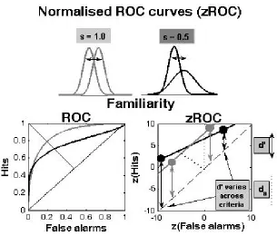
2.2.2. Receiver Operating Characteristic ... 68
2.2.3. Sensitivity measures (d’, da, Az) ... 75
2.2.4. Bias measures (Xi,c,ca)... 78
2.3. DATA ANALYSIS... 80
2.3.1. Raw measures ... 80
2.3.2. Derived measures... 82
2.3.3. Power analysis ... 89
2.3.4. Regressions (zROC) ... 92
CHAPTER 3. EXPERIMENTS 1-4 ... 94
3.1. INTRODUCTION... 94
3.2. EXPERIMENT1: ENCODING TASK,LONG INTERVAL, 3X... 95
3.2.1. Methods ... 95
3.2.2. Results ... 99
3.2.3. Discussion ... 103
3.3. EXPERIMENT2: LURE TYPE,LONG INTERVAL, 3X... 105
3.3.1. Methods ... 106
3.3.2. Results ... 108
3.3.3. Discussion ... 113
3.4. EXPERIMENT3: LURE TYPE,SHORT INTERVAL, 3X,ENC.TASK... 113
3.4.1. Methods ... 114
3.4.2. Results ... 115
3.4.3. Discussion ...122
3.5. EXPERIMENT4: LURE TYPE,RETENTION INTERVAL, 6X...124
3.6. DISCUSSION OFEXPERIMENTS1TO4... 138
3.6.1. Empirical summary ... 138
3.6.2. Relation to other length and strength studies ... 140
3.6.3. Implications for memory models... 142
3.6.4. Limitations ... 145
CHAPTER 4. EXPERIMENTS 5-7 ... 147
4.1. INTRODUCTION... 147
4.2. EXPERIMENT5A: RETENTION INTERVAL,WITHOUT NEW, 3X,ONE... 148
4.2.1. Methods ... 150
4.2.2. Results ... 154
4.2.3. Discussion ... 159
4.3. EXPERIMENT5B: RETENTION INTERVAL,WITHOUT NEW, 3X,TWO... 160
4.3.1. Methods ... 161
4.3.2. Results ... 161
4.3.3. Discussion ... 171
4.4. EXPERIMENT6: RETENTION INTERVAL,WITHOUT NEW, 6X,TWO... 174
4.4.2. Methods ... 177
4.4.3. Results ... 178
4.4.4. Discussion ... 188
4.5. EXPERIMENT7: RETENTION INTERVAL,LURE TYPE,WITH NEW, 6X... 193
4.5.1. Methods ... 195
4.5.2. Results ... 196
4.5.3. Discussion ... 204
4.6. DISCUSSION OFEXPERIMENTS5TO7... 207
4.6.1. Empirical summary ... 207
4.6.2. Relation to other experiments ... 210
4.6.3. Implications for memory models... 214
4.6.4. Limitations ...234
CHAPTER 5. GENERAL DISCUSSION ...238
5.2. THE ROLE OF RETRIEVAL PRACTICE... 242
5.3. FURTHERDIRECTIONS... 244
5.3.1. Cued recall ... 244
5.3.2. Associative recognition ... 249
REFERENCES... 251
APPENDIX 1 ... 269
EXPERIMENT1 ... 269
EXPERIMENT2 ... 271
EXPERIMENT3 ... 272
EXPERIMENT4 ... 275
EXPERIMENT5A... 278
EXPERIMENT5B... 281
EXPERIMENT6 ... 284
EXPERIMENT7 ... 287
APPENDIX 2 ... 290
EXPERIMENT1 ... 290
EXPERIMENT2 ... 291
EXPERIMENT3 ... 291
EXPERIMENT4 ... 291
EXPERIMENT5A... 292
EXPERIMENT5B... 293
EXPERIMENT6 ... 295
EXPERIMENT7 ... 296
FIGURE1.1. SIGNAL DETECTION INTERPRETATION OF RECOGNITION MEMORY... 4
FIGURE1.2. BINDCUEDECIDEMODEL OFEPISODICMEMORY(BCDMEM). ... 39
FIGURE1.3. SOUCE OFACTIVATIONCONFUSION(SAC)MODEL. ... 44
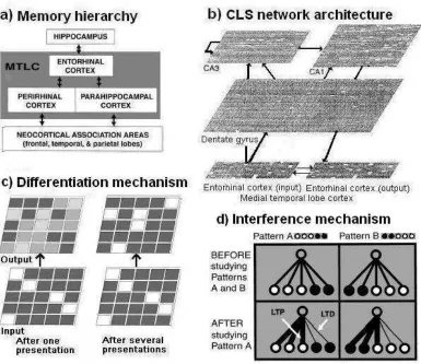
FIGURE1.4. COMPLEMENTARYLEARNINGSYSTEMS(CLS)MODEL. ... 50
FIGURE2.1. UNEQUAL VARIANCESDTMODEL AND SENSITIVITY MEASURE. ... 67
FIGURE2.2. EQUAL VARIANCESDTMODEL AND THEROCCURVE. ... 69
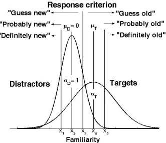
FIGURE2.3. EQUAL VARIANCESDTMODEL WITH FIVE RESPONSE CRITERIA... 71
FIGURE2.4. CONSTRUCTION OFROCCURVE FROM FREQUENCY DATA... 73
FIGURE2.5. EFFECT OF CRITERION SHIFTS ON SINGLE-POINT SENSITIVITY. ... 77
FIGURE2.6. UNEQUAL-VARIANCESDTMODEL ESTIMATED BYRSCOREPLUS. ... 84
FIGURE3.1. DESIGN OFEXPERIMENT1. ... 97
FIGURE3.2. WORD-FREQUENCY EFFECT ACROSS LIST TYPES(EXP. 1). ... 101
FIGURE3.3. ROCCURVES FOREXPERIMENT1... 103
FIGURE3.4. DESIGN OFEXPERIMENT2. ... 107
FIGURE3.5. WORD-FREQUENCY EFFECT ACROSS LIST TYPES(EXP. 2). ... 109
FIGURE3.6. ROCCURVES FOREXP. 2... 111
FIGURE3.7. DESIGN OFEXPERIMENT3. ... 115
FIGURE3.8. ROCCURVES FOREXP. 3... 119
FIGURE3.9. SENSITIVITY ACROSS RETENTION INTERVALS(EXPS. 2 / 3). ... 122
FIGURE3.10. DESIGN OFEXPERIMENT4. ... 126
FIGURE3.11. SENSITIVITY ACROSS COMPARISON TYPES(EXP. 4)... 129
FIGURE3.12. ROCCURVES ACROSS RETENTION INTERVALS(EXP. 4). ... 130
FIGURE3.13. SENSITIVITY ACROSS NUMBER OF REPETITIONS(EXPS. 3 / 4). ... 133
FIGURE4.1. DESIGN OFEXPERIMENT5. ... 152
FIGURE4.2. ROCCURVES FORAANDBITEMS(EXP. 5A)... 158
FIGURE4.3. ROCANDZROCCURVES FORAANDBITEMS(EXP. 5B). ... 166
FIGURE4.4. SENSITIVITY ACROSS NUMBER OF SESSIONS(EXPS. 5A/ 5B). ... 169
FIGURE4.5. DESIGN OFEXPERIMENT6. ...177
FIGURE4.6. ROCCURVES ACROSS RETENTION INTERVALS(EXP. 6). ...184
FIGURE4.7. SENSITIVITY ACROSS REPETITIONS AND ITEM TYPES(EXPS. 5B/ 6)..187
FIGURE4.11. SENSITIVITY ACROSS RETENTION INTERVALS(EXPS. 6-A/ 7-SSP).204
TABLE3.1. HITS AND FALSE ALARMS(EXP. 1). ... 100
TABLE3.2. SENSITIVITY(AZ)AND BIAS(CA) (EXP. 1). ... 102
TABLE3.3. HITS AND FALSE ALARMS(EXP. 2). ... 108
TABLE3.4. SENSITIVITY(AZ)ACROSS DISCRIMINATION TYPES(EXP. 2). ... 110
TABLE3.5. BIAS(CA)ACROSS DISCRIMINATION TYPES(EXP. 2). ... 112
TABLE3.6. HITS AND FALSE ALARMS ACROSS ENCODING TASKS(EXP. 3)... 116
TABLE3.7. SENSITIVITY(AZ)ACROSS DISCRIMINATION TYPES(EXP. 3). ... 118
TABLE3.8. BIAS(CA)ACROSS DISCRIMINATION TYPES(EXP. 3). ... 121
TABLE3.9. HITS AND FALSE ALARMS(EXP. 4). ... 127
TABLE3.10. SENSITIVITY(AZ)ACROSS DISCRIMINATION TYPES(EXP. 4). ... 128
TABLE3.11. BIAS(CA)ACROSS DISCRIMINATION TYPES(EXP. 4). ... 132
TABLE4.1. HITS AND FALSE ALARMS ACROSS ITEM TYPES(EXP. 5A)... 155
TABLE4.2. SENSITIVITY(AZ; SSPCOMPARISON)ACROSS ITEM TYPES(EXP. 5A).157 TABLE4.3. BIAS ACROSS ITEM TYPES(CA) (EXP. 5A)... 159
TABLE4.4. HITS AND FALSE ALARMS ACROSS ITEM TYPES(EXP. 5B)... 162
TABLE4.5. SENSITIVITY(AZ; SSPCOMPARISON)ACROSS ITEM TYPES(EXP. 5B).165 TABLE4.6. BIAS ACROSS ITEM TYPES(CA) (EXP. 5B)... 167
TABLE4.7. HITS AND FALSE ALARMS ACROSS ITEM TYPES(EXP. 6). ... 181
TABLE4.8. SENSITIVITY(AZ; SSPCOMPARISON)ACROSS ITEM TYPES(EXP. 6). . 183
TABLE4.9. BIAS ACROSS ITEM TYPES(CA) (EXP. 6). ... 185
TABLE4.10. SENSITIVITY(D’)INCARY ANDREDER(2003). ... 189
TABLE4.11. HITS AND FALSE ALARMS INNORMAN(1999)... 190
TABLE4.12. HITS AND FALSE ALARMS(EXP. 7). ... 197
TABLE4.13. SENSITIVITY(AZ)ACROSS RETENTION INTERVALS(EXP. 7). ... 199
TABLE4.14. BIAS(CA)ACROSS DISCRIMINATION TYPES(EXP. 7). ... 203
TABLE4.15. EFFECT SIZES OFLLES ANDLSES(EXP. 7)... 205
LLE List-Length Effect
LSE List-Strength Effect
Short Short list (all weak items; presented once)
Long Long list (all weak items)
Strong Strong list (half weak items; half strong items)
H Hit rate (proportion of correct “old” responses)
F False-alarm rate (proportion of incorrect “old” responses)
μ Mean familiarity for target (μT)and distractor (μD) distributions
σ Standard deviation for target (σT) and distractor (σD) distributions
M Sample mean
SD Sample standard deviation
N Number of participants
SEM Standard error of the mean (= SD/ N )
d’ Discriminability (when distributions have equal variance)
da Discriminability (when distributions have unequal variance)
Xi Decision criterion (i= 1 to 6)
c Decision criterion (equal variance)
ca Decision criterion (unequal variance)
Φ(X) Cumulative normal distribution (X= value of random variable)
z(P) Inverse cumulative normal distribution (P= proportion)
ROC Receiver Operating Characteristic curve (y= hits,x= false alarms)
zROC Normalised ROC [y=z(H),x=z(F)]
Az Area under ROC, normal distribution assumed
BCDMEM Bind Cue Decide Model of Episodic Memory
CLS Complementary Learning Systems model
SAC Source of Activation Confusion model
SAM Search of Associative Memory model
REM Retrieving Effectively from Memory model
This thesis is the work of the author and has not been submitted for a degree at
another university. Portions of Chapter 3 (Experiment 3 in section 3.4) have been
published in Buratto, L. & Lamberts, K. (2008). List-strength effect without
list-length effect in recognition memory.Quarterly Journal of Experimental
There are many people who have helped me immensely at different stages of this
project. I would like to thank Nick Chater for bringing me to Warwick and Koen
Lamberts for “adopting” me after Nick left for University College London. Koen
has been a constant source of support and wise advice throughout this period and
I consider myself lucky to have inadvertently ended up under his supervision.
I would like to thank Menelaos Apostolou, Elizabeth Blagrove, Duncan Guest,
William Jimenez-Leal, Chris Kent, William Matthews, Kerry McColgan, Joanne
Myers, Erika Nurmsoo, Maria Sapouna, Christoph Ungemach, and Theodora
Zarkadi for making my stay at Warwick a much more enjoyable experience.
I also would like to thank the British government and Warwick University’s
Department of Psychology for providing me with funding (Overseas Research
Students Award Scheme and Warwick Postgraduate Research Fellowship,
respectively), which allowed me to work during these three-and-a-half years
without financial worries.
Finally, I am greatly indebted to my parents, Paulo and Julieta, who always
encouraged me to study (in good faith, I would say, as they have only a vague
idea of what I am up to!), my brother, Gabriel, for his friendship and for
providing me with constant motivation for spelling out clearly any ideas I might
have, and my wife, Noeli, who has been by my side through it all, for her
The study of interference effects is important to constrain models of memory.
List-length manipulations test how adding new information to memory affects
memory for the other stored information (list-length effect; LLE). List-strength
manipulations test how strengthening some information in memory affects
memory for the other non-strengthened information (list-strength effect; LSE).
Whereas LLE and LSE are generally found in recall tasks, their empirical status
in recognition tasks is less well established. In this thesis, we investigated some
boundary conditions for both list-length and list-strength effects. The results
provided evidence for the following claims:i) LLE and LSE are real effects in
recognition (the effects were obtained after controlling for several confounds);ii)
LLE and LSE are modulated by the relative contribution of recall-like processes
operating at test (more recollection at test yielded larger effects);iii) LLE and
LSE can be modulated by the number of study-test blocks in an experimental
session (fewer study-test blocks resulted in larger effects); iv) LLE and LSE can
be modulated by the time interval between study and test (shorter intervals
produced larger effects) and iv) LLE and LSE may not be strongly modulated by
the magnitude of length and strength manipulations (stronger manipulations did
not result in larger effects). Taken together, the results support memory models
that attribute forgetting in recognition to competition between memory traces
during either encoding or retrieval. The results provide little support for models
that attribute forgetting solely to interference between the contexts in which a
Chapter 1.
Review and objectives
How is education supposed to make me feel smarter? Every time I learn something new, it pushes some old stuff out of my brain. Remember when I took that home winemaking course, and I forgot how to drive? Homer Simpson
1.1. Introduction
The study of interference is an important element of memory research. Is it the
case that the more one learns, the more one forgets? Is it the case that learning
something well comes at the cost of forgetting something else? In this thesis, we
focus on how memories interact when people undergo recognition tests, where
the task is to distinguish whether or not a given piece of information has been
previously seen. In particular, we are interested in what happens to the memory
of a given piece of information when many new pieces of information are learned
once or when few new pieces of information are learned over and over again.
In this type of research, “piece of information” is usually represented by a
“word” and the “contents of memory” are represented by a “list of words”. Two
manipulations have been commonly used to assess interference in memory:
list-length and list-strength manipulations. List-list-length manipulations test how adding
items to a list of words affects memory for the other words on the list. A
list-length effect (LLE) involves better performance on short lists than on long lists.
List-strength manipulations, on the other hand, test how strengthening items
(e.g., by repetition or study time) affects memory for the other, non-strengthened
items on the list. A list-strength effect (LSE) occurs when performance on
non-strengthened items is better inpure weaklists (where all items have the same
strength) than inmixedlists (where some items have been strengthened).
Length and strength manipulations areempiricallyinteresting because they allow
us to evaluate how stored items affect each other during memory tasks. Those
manipulations are alsotheoreticallyimportant because they test core assumptions
of several computational memory models. Indeed, a whole class of models – the
items stored in memory interfere with each other during storage or retrieval. This
type of interference could potentially explain why forgetting occurs.
Although global matching models predict LLE and LSE, and although the
existence of such effects could be almost taken for granted (i.e., it is intuitive to
think that adding items to a list should impair the memory of any one item),
empirical results in recognition studies have been mixed. Both positive and null
LLEs and positive and null LSEs have been reported. Those findings represent a
challenge to established memory models. Indeed, new memory models have been
developed in recent years trying to explain the mixed pattern of results.
Given the uncertain status of length and strength effects in recognition and given
their theoretical importance, it is crucial to carefully investigate the boundary
conditions underlying those effects. The main aim of this thesis is to present
evidence bearing on such boundary conditions. In this chapter, we describe why
length and strength manipulations are theoretically important. Next, we introduce
the list-length and list-strength paradigms (and their variations) and review the
main empirical findings, discussing some limitations of previous research.
1.2. Early global matching memory models
In the 1980s, several process models were developed that were able to account
for findings in a wide range of experimental paradigms, including categorisation,
recall and recognition (hence the nameglobal models). We will focus on the
three most investigated models from that generation: Search of Associative
Memory (SAM; Gillund & Shiffrin, 1984), MINERVA2 (Hintzman, 1988) and
TODAM (Theory of Distributed Associative Memory; Murdock, 1982).
Although differing in many respects, those models share two common
assumptions when applied to recognition memory: they assume that all items
stored in memory contribute information to the recognition decision and that the
information contributed by each item in memory is evaluated in parallel. In other
words, when an item is presented at test, the information used to assess whether
from all items stored in memory. This information signal can be interpreted as an
index of thematchbetween the test items and the contents of memory (hence the
namematching models), or alternatively, as an index of thefamiliarityof the test
item. Thus the more familiar a test item, the higher the familiarity signal.
The matching assumption allows SAM, MINERVA2 and TODAM to explain
phenomena that were difficult for previous models to account for, namely, the
speed of recognition decisions and similarity effects. High confidence memory
decisions are made fast (Glucksberg & McCloskey, 1981); matching models can
account for that through the parallelism of the matching process. Matching
models can also account for similarity effects – the finding that false recognitions
are high when the items stored in memory are similar to each other and to the test
item (e.g., Posner & Keele, 1970) – because they take into account all stored
items during the recognition process.
The familiarity signal produced by the matching process can then be analysed
within the framework of Signal Detection Theory (SDT; Macmillan & Creelman,
2005). The familiarity of a given class of items (e.g., high-frequency words,
concrete words) is assumed to follow a normal distribution with meanμand
standard deviationσ(a more detailed description of SDT applied to recognition
memory is given in Chapter 2). The familiarity distribution of studied items (also
calledtargetorolditems)is assumed to have higher mean and standard
deviation than the distribution of unstudied items (also calleddistractor,new,foil
orlureitems). Performance at this level of analysis is thus a function of the
means and standard deviations oftarget(μT,σT) anddistractor(μD,σD)
distributions. Global matching models are able to produce estimates of means
and standard deviations, and those estimates are used to predict recognition
performance. One commonly used measure of discriminability is given by:
' T D
T
d
(1.1)
In other words, the ability to discriminate studied from unstudied items is
proportional to the difference between the means oftargetsandluresand
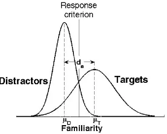
inversely proportional to the standard deviation of thetargetdistribution. Figure
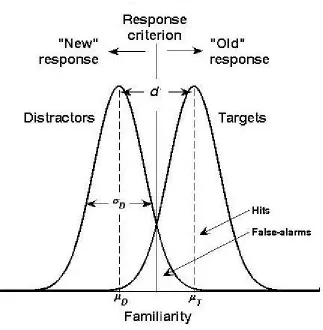
Figure 1.1. Signal detection interpretation of recognition memory.
The decision axis represents the familiarity scale, ranging from low to high. The two Gaussian distributions represent familiarities associated with targets (meanμT) and distractors (meanμD;
standard deviationσD). Standard deviations are assumed to be equal. Discriminabilityd’is the
standardised difference between the means of targets and distractors. The vertical bar (criterion) separates the decision space between “old” responses (i.e., “I have seen the item”) and “new” responses (i.e., “I have not seen the item”). Hits represent the proportion of “old” responses given to targets; false alarms represent the proportion of “old” responses given to distractors.
Because global matching models take into account information about other items
in memory during the matching process, it is possible that the memory of a given
target item is impaired by manipulations affecting the remaining items in
memory (e.g., adding items to memory or strengthening some items in memory).
SAM, MINERVA2 and TODAM all predict a decrease in discriminability (d’) as
a result of list-length and list-strength manipulations. In the following, we briefly
describe those models and explain why they predict LLE and LSE (for a review
1.2.1. SAM (Gillund & Shiffrin, 1984)
In this model, memory is represented as a matrix of association strengths
between memory traces and the cues used to activate those traces. Associations
are generated during learning through a rehearsal process modulated by four
parameters:amodulates the association strength between study context and
study item (contextual association);bmodulates the association between items
that were studied together (inter-item association);cmodulates the association
between a studied item and its own trace; anddmodulates the association
between a studied and a non-studied item (i.e., pre-experimental association).
Because traces in SAM are stored separately from each other, interference does
not occur at storage. Instead, forgetting is due to events unfolding at the time of
retrieval. During the retrieval process, a familiarity signal is produced through
the activation of all stored memories by the cues available at test (i.e., the test
context and the test item). IfCrepresents the test context cue andIrepresents the
item cue, then the familiarity signal elicited by a test itemIis given by
1
( , ) ( , ) C ( , ) I
N
W W
j j
j
F C I S C I S I I
(1.2)whereNis the number of traces in memory,WCandWIare attention weights
(e.g.,WC=WI= 0.5) andS(X,Y) are the association strengths between cueXand
memory traceY. To illustrate, if the cueCis the test context, thenS(C,Ij) =a, and
if cueI represents traceIj stored in memory, thenS(I,Ij) =c. Equation 1.2
implements the matching assumption, since familiarity is obtained by summing
over all traces stored in memory. To produce a response, the model compares the
familiarity signal to a decision criterion: if the signal is higher than the criterion,
then an “old” response is produced. Otherwise, a “new” response is produced.
In order to avoid perfect performance, variability is added to the association
strengthsa,b,candd. The assumption adopted by Gillund and Shiffrin (1984)
involved replacing each strengthXin the memory matrix with a value taken from
a 3-point uniform distribution given by 0.5XorXor 1.5X. As a result, the means
and variances of associative strength distributions are tied in the SAM model: the
List-length and list-strength effects follow from SAM’s variability assumptions.
As shown in Equation 1.1, discriminability is a function of two factors: the
difference in the mean familiarity values of targets and distractors (numerator);
the size of the distractor variance (denominator). The numerator is not affected
by length or strength: adding items or strengthening some items increments the
mean familiarity of both targets and distractors by the same amount (see Clark &
Gronlund, 1996, p. 41, for an example). The denominator, however, is predicted
to increase. The terms in the summation in Equation 1.2 are independent (by
assumption) and it is known from probability theory that the variance of the sum
of independent variables is the sum of their variances. Thus adding more items to
a list increases both target and distractor variances (moreS(C,Ij)×S(I,Ij) =ad
terms are added to the familiarity of both distributions). Similarly, strengthening
some items increases the values of parameterafor those items (the association
between strong items and context is higher than the association between weak
items and context), and higheraimplies higher variance. The increase in
variability (denominator in Equation 1.1) causes performance (d’) to decrease. In
sum, the SAM model predicts both list-length and list-strength effects in
recognition, and these predictions follow from core assumptions of the model.
1.2.2. MINERVA2 (Hintzman, 1988)
Memory traces are represented as separate vectors containingMfeatures. Each
feature can assume values +1, 0 or -1. Features of study items are correctly stored
with probabilityL(0 is stored with probability 1 –L). Variability in the matching
process comes from the probabilistic nature of feature encoding. The familiarity
signal produced by a test item is obtained by taking the dot product of the test
item with each vector stored in memory. IfTrepresents a stored vector andP
represents the test vector, then the familiarity elicited byPat test is given by
3
1 1 ,
( )
N M
ij j
i j i
T P F P
N
(1.3)whereNis the number of traces in memory,Tijis the value of featurejin tracei,
Pjis the value of featurejin the test item andN±,jis the number of non-zero
the model to boost the signal produced by test cues that are similar to stored
traces and shrink the signal from cues that are dissimilar to stored traces. The
familiarity signal is then compared to a criterion in order to output a response.
Like SAM, MINERVA2 predicts the occurrence of list-length and list-strength
effects at retrieval due to an increase in the variance of familiarity distributions.
The mean difference between targets and distractors does not change because, for
each non-target trace activated by an old test item, there is an equivalent
activation of that trace by a new test item. By contrast, the variance increases
with longer and stronger lists because each stored trace is an independent and
additive source of variance to the familiarity signal (the encoding probabilityLis
applied independently to each feature of each trace). Thus MINERVA2 also
predicts both list-length and list-strength effects in recognition.
1.2.3. TODAM (Murdock, 1982)
In TODAM, each item is represented by a vector ofNfeatures. Features are
either encoded (probabilityp) or not encoded (set to 0 with probability 1 –p).
Each feature value is chosen from a distribution with mean 0 and variance 1/N.
All items are stored in a common vector. Thus, unlike SAM and MINERVA2,
where traces are stored separately, representation in TODAM is composite.
Consequently, forgetting is assumed to occur at storage.
IfMi-1is the composite vector containingi–1 traces andfiis a new trace, then the
updated version ofMi-1is given byMi=αMi-1+ pfi, whereα(< 1) is a forgetting
parameter (i.e., before encodingfi,Mis decremented byα). The familiarity signal
associated with test itemgis produced in TODAM by taking the dot product
between test itemgand the memory vectorM, such that:
1 ( )
N
i i
i
F g g M g M
(1.4)Ifgmatches a trace in memory (i.e., a vector that was added to the composite
vectorM), then the mean familiarity of that match ispαL-i, whereLis the list
length andiis the serial position where itemgwas studied. If the test item does
not match any trace encoded inM, then the mean familiarity is 0. The variance of
Weber, 1988, Table 1). Thus higher encoding probabilityp(obtained by item
repetition, for example) entails higher variance. Like SAM and MINERVA2, the
outcome of the matching process is compared to a decision criterion in order to
emit an old-new response.
TODAM predicts LLE because the familiarity of each item is decreased for
every new item added to the list (i.e., match =pαL-i). Moreover, every extra item
adds another source of variance. Thus the numerator of Equation 1.1 decreases
and the denominator increases, resulting in a decrease ind’. TODAM predicts
LSE because stronger lists have higher mean variances than weaker lists.
1.3. Empirical evidence: early studies
The global matching models discussed in the previous section predict list-length
and list-strength effects in recognition. But what is the evidence supporting those
predictions? Here we review some early studies suggesting that LLE is a real
phenomenon in recognition whereas LSE is not.
1.3.1. Evidence for list-length effect
List-length effect has long been observed in recall (e.g., Ebbinghaus, 1885/1964;
Murdock, 1962) and recognition (e.g., Strong, 1912) and has thus been treated as
a standard phenomenon to be explained by any memory model.
In his seminal study, Strong (1912) asked participants to study sequences of
full-page advertisements. The sequences contained 5 to 150 advertisements. At test,
old and new items were presented and participants had to sort each advertisement
into piles according to confidence. The results showed thathit rates(proportion
of correct “old” responses) decreased with list length andfalse alarm rates
(proportion of incorrect “old” responses) increased with list length.
Strong’s (1912) study, however, confounded list length with study-test lag.1The test was carried out immediately after study in both the short and long conditions.
As a consequence, the average study-test lag per item was shorter in the short list
than in the long list. Because recognition drops with longer lags (e.g., Shepard,
1967; Strong, 1913), either list length or study-test lag could have accounted for
the results. Another confound refers to the size of the test list. Longer study lists
were followed by longer test lists. But it is known that discrimination on the
latter part of a long list is impaired relative to discrimination at the beginning of
the list (Schulman, 1974). Thus average performance in a long test list is worse
than in a short test list, regardless of the length of the study list. Finally, Strong’s
(1912) study did not control for serial position effects. Items at the beginning and
at the end of a list are better recognised than items in the middle (Neath, 1993;
Schulman, 1974). This primacy and recency advantage would benefit short lists
more than long lists because a higher proportion of items in the short list would
partake of the gain.
Several subsequent studies continued to confound list length with other variables
(e.g., length of test list in Murnane & Shiffrin, 1991a; study-test lag in Yonelinas,
1994). But the effect was still observed even when most of those confounds were
eliminated. Gronlund and Elam (1994), for example, found a strong and reliable
LLE when using aretroactive design. This experimental design addressed early
criticisms because it equated study-test lag between short and long conditions
(the period after the presentation of study items was filled with a distractor task)
and because it controlled for serial position effects (only items studied at the
beginning of both lists were compared).2
Despite the apparent reality of LLE in recognition, Murdock and Kahana (1993a,
1993b) argued that the effect should disappear when the number of items
intervening between study of an item and its test is controlled. This prediction
was derived from a modified version of TODAM proposed to account for the
absence of LSE in recognition (see 1.3.2 and 1.4.2). In most studies, targets on
the study list and targets and distractors on the test list are randomly mixed. Thus
it is usually not possible to assess directly the effect of the number of intervening
2The fact that only early items in both study lists enter the analysis suggests that any ensuing
items on memory. To address this issue, Ohrt and Gronlund (1999, Exp. 1)
conducted an experiment using aproactive design. In this design, study-test lag
is equated (the period after the end of both lists is filled with a distractor task),
serial position effects are controlled (only items studied at the end of both lists
are compared) and the number of intervening items is taken into account (items
studied early are tested early; items studied late are tested late).3Unlike the retroactive design, where the distractor task is longer in the short list than in the
long list, the proactive design requires equal distractor times for both list lengths.
Ohrt and Gronlund (1999) found a significant LLE. The effect was replicated in a
second experiment where category length was manipulated and study-test
positions were controlled. These results, together with the results of similar
studies (e.g., Ratcliff, McKoon, & Tindall, 1994, Exp. 3), suggest that the LLE is
not an experimental artifact; apparently it represents a real phenomenon.
1.3.2. Evidence against list-strength effect
Unlike list-length manipulations, which have been studied since Ebbinghaus in
the late 1800s, list-strength manipulations have attracted attention only during
the last 30 years. Tulving and Hastie (1972), the first to investigate the issue,
found an LSE in free recall (see also Malmberg & Shiffrin, 2005; Ratcliff, Clark,
& Shiffrin, 1990, Exp. 6; Rose & Sutton, 1996; Wixted, Ghadisha, & Vera,
1997). Most studies up until the end of the 1990s, however, have found only a
small LSE in cued recall (Ratcliff, Clark, & Shiffrin, 1990, Exps. 3 and 6) and no
effect in recognition at all (Hirshman, 1995; Murnane & Shiffrin, 1991a, 1991b;
Ratcliff et al., 1990; Ratcliff, Gronlund, & Sheu, 1992; Ratcliff et al., 1994;
Yonelinas, Murdock, & Hockley, 1992).
Strength manipulations have usually been implemented using themixed-pure
paradigm(Ratcliff et al., 1990). Participants are presented withmixed lists
containing weak items (e.g., presented once or for a short time) and strong items
(e.g., presented more than once or for a longer time). As the goal is to assess the
impact strengthening some items has on non-strengthened items, it is necessary
3As only late items in both study lists enter the analysis, any forgetting is likely to have been
to create appropriate controls against which to compare the performance of weak
and strong items in the mixed lists. There are two possible controls:pure weak
listsare lists containing only weak items andpure strong listscontain only strong
items. The number of unique items in each list is held constant to control for
list-length effects. A list-strength effect occurs if:i) weak item discrimination is
better inpure weaklists than inmixedlists;ii) strong item discrimination is
better inmixedlists than inpure stronglists.
Ratcliff et al. (1990) conducted 7 experiments, none of which showed the
predicted differences between pure and mixed lists. Moreover, in their
Experiment 6, list length was manipulated along with list strength and the results
yielded a dissociation whereby LLE was observed and LSE was not. Null results
are difficult to interpret in general (Frick, 1996) and because this particular result
(null LSE) has serious implications for global matching models, it is important to
make every possible effort to rule out confounds in the experimental design.
One important confound in designs using mixed lists isrehearsal redistribution,
which occurs when participants take effort or rehearsal time away from strong
items in a mixed list and redistribute that effort or time to weak items in the same
list. This may occur because after a few presentations of the same word,
participants may feel they already know the item well enough and that they
should spend some time practicing other less-well-learned items. To the extent
that this rehearsal redistribution occurs, it works against the possibility of finding
an LSE, as weak items would receive more rehearsal time (and become stronger)
and strong items would receive less rehearsal time (and become weaker).
Therefore, any differences between weak and strong items across pure and mixed
lists would be reduced and could potentially disappear. Although rehearsal
redistribution can occur in pure lists (either weak or strong), it does not work
against finding an LSE in those lists because any rehearsal taken away from an
item is reallocated to another item of the same class.
Several studies converged on the conclusion that rehearsal redistribution was not
the reason behind the null LSE. For example, Ratcliff et al. (1990) blocked weak
occurred at the block boundaries); Murnane and Shiffrin (1991b) analysed their
data as a function of the strength of a given item’s neighbours (assuming that
redistribution occurs mainly between adjacent items); Yonelinas et al. (1992)
presented words for very short periods of time (50 ms for weak items; 200 ms for
strong items), under the assumption that rehearsal strategies take time and that
during such short presentation times participants would not have enough time to
read the word and simultaneously adopt a redistribution strategy. In all these
studies, where rehearsal redistribution was unlikely to operate, no LSE emerged.4
The experimental confounds present in early list-length experiments (see 1.3.1)
were also present in early list-strength experiments (e.g., study-test lag in
Yonelinas et al., 1992). Stronger lists are also longer in total presentation time.
Therefore, a study-test lag confound should work towards finding an LSE
because weak items in weak lists would have a shorter study-test lag, on average,
than weak items in mixed lists and strong items in pure lists would have a longer
study-test lag than strong items in mixed lists. The fact that an LSE was not
found even in experiments containing study-test lag confounds can be interpreted
as support for the null finding. In any case, when study-test lag was controlled
for, the results unsurprisingly showed no sign of an LSE (e.g., Murnane &
Shiffrin, 1991a, Exps. 3 and 6).
The only visible effect of the list-strength manipulation on mixed-list items was
observed in the setting of thedecision criterion. The criterion corresponds to the
cut-off value in familiarity space that separates “old” from “new” responses. It
represents the minimum degree of familiarity elicited by a test item that a
participant deems sufficient to emit an “old” response. Hirshman (1995) found
that criterion placement varied systematically with list strength: it increased from
pure weaktomixedtopure stronglists, indicating that participants became more
and more conservative in their output of “old” responses as average item strength
4Murnane and Shiffrin (1991b) found an LSE only when items were likely to be stored
increased. Hirshman (1995) found this pattern not only in his experiments but
also in most previously published list-strength studies (the pattern held in 75 out
of 92 comparisons between conditions).
Criterion can be estimated by observing the behaviour of hits and false alarms
across conditions. If hits and false alarms move in the same direction (i.e., they
increase or decrease in tandem), then one may claim a criterion shift occurred.5 Criterion setting is assumed to be under the participants’ strategic control. But
because no instructions expected to affect criterion setting are usually given to
participants in list-strength experiments, criterion has been treated by global
matching models simply as a parameter to be estimated, without any real
mechanism accounting for its behaviour. For our present purposes, it suffices to
say that, unlike list-length manipulations, where criterion setting rarely changes
between conditions (hits and false alarms move in opposite directions),
list-strength manipulations tend to cause criterion shifts across pure and mixed list
conditions (hits and false alarms decrease in tandem).
Because list-strength manipulations affect criterion setting across conditions, and
because criterion setting may have an effect in discriminability measures such as
d’(see Van Zandt, 2000, for recent evidence), it is important to control criterion
placement in any demonstration of a null LSE. To address this issue, Shiffrin,
Huber and Marinelli (1995) used long lists of categorised items. Participants are
reluctant to change the decision criterion within the same list, especially when no
feedback is provided after each trial (Stretch & Wixted, 1998b; Verde & Rotello,
2007). Length was manipulated by increasing the number of items in a category
and strength was manipulated by increasing the number of presentations of an
item in a category. As expected, criterion did not change across conditions (false
alarms for weak and strong items were the same for pure and mixed categories).
More importantly, the results revealed a positive LLE but no LSE.
In short, the results of several studies carried out up until the end of the 1990s
were consistent with the idea that there is no list-strength effect in recognition.
5Unidirectional changes in hits and false alarms can also be caused by a shift in the underlying
Those results represented a challenge to global matching models, since they all
predicted the existence of an LSE directly from their basic assumptions.
1.3.3. Other challenges to global matching models
The null LSE was not the only challenge faced by global matching models at that
time. Other results also started to cast doubt on some of the models assumptions.
Here we discuss a series of results that went counter to the predictions made by
the global models SAM, MINERVA2 and TODAM.
As discussed in 1.2, global matching models predict that the variance of old and
new items should increase with increases in list length and list strength. In
particular, SAM and MINERVA2 predicted that item strength should increase
the variance of the old-item distribution more than the variance of the new-item
distribution. That should occur because the match value of an old test item
depends on how strongly that item was encoded in memory: the higher the
strength in memory, the higher the match value.
An old test item matches one trace in memory and mismatches all the other
traces, whereas a new test item mismatches all traces in memory. When the
match value of an old item increases, the contribution to the overall old-item
variance starts to be dominated by the value of the strong match over the values
of all the mismatches. The variance of new-item distribution, on the other hand,
contains only the contribution of mismatches. Therefore, the variance of old
items should increase relative to the variance of new items when strength is
manipulated. In TODAM, by contrast, the variances of old and new distributions
should not appreciably change, as the variance of a match is about twice the
variance of a mismatch, regardless of strength. Thus the new-to-old variance
ratio should either decrease with list strength (ratio less than 1, according to
SAM and MINERVA2) or remain constant (ratio equal to 1, according to
TODAM). Ratcliff, Gronlund and Sheu (1992) found a constant variance ratio,
disconfirming the predictions of the three models.6
6Ratcliff et al.’s (1992) estimate of the new-to-old standard deviation ratio was 0.8. In Chapter 2,
we describe how standard deviation ratios (s=σD/σT) and, consequently, variance ratios can be
Subsequent studies confirmed the finding and extended it to list-length
manipulations. When list length increases, the number of traces encoded in
memory also increases. This leads to an increase in the variance of old and new
item distributions as there are more independent terms added to the familiarity
sum. As the list length increases, the contribution of mismatches to the overall
variance of the old distribution starts to dominate the contribution of matches.
Similarly, the new-item variance is made up exclusively of mismatches. Thus, as
list length increases, the new-to-old variance ratio should approach 1. This
prediction is shared by SAM, MINERVA2 and TODAM. Contrary to the
prediction, Gronlund and Elam (1994, Exp. 1) and Ratcliff et al. (1994, Exp. 3)
found that the variance ratio was constant across list lengths and set around 1.
The fact that the estimated new-to-old variance ratios were constant across
list-length and list-strength manipulations contradicted core assumptions of the
global matching models. Because those assumptions underlay most of the
published predictions for those models, major revisions became necessary.
1.4. Recent global matching memory models
The challenges presented to global matching models following their failure to
predict several patterns of results led to changes in some of their basic
assumptions and led to the development of a new generation of matching models,
including REM (Shiffrin & Steyvers, 1997) and SLiM (McClelland & Chappell,
1998). In the following, we describe the modifications implemented in the early
matching models to account for the null LSE, how those modifications were
incorporated into REM and how they affected the predictions for LLE and LSE.
1.4.1. SAM and the differentiation assumption
In SAM, the strength parameterdrepresenting the association between a lure test
item and a trace in memory (i.e., a form of pre-experimental associative strength)
is assumed to be constant, regardless of trace strength. The parametera
(contextual strength), on the other hand, increases with trace strength. Thus
strength is increased. If insteaddis assumed to decrease when the strength of the
memory traces increases, then a form ofdifferentiationhas been implemented: as
a trace becomes stronger, it becomes more connected to the study context
(increase ina) and less connected to unstudied items (decrease ind). In other
words, strong items become increasingly distinct from weak items. And because
the new-item variance remains largely unchanged, an LSE is not predicted (see
Shiffrin, Ratcliff, & Clark, 1990, for a detailed discussion). Conversely, an LLE
is still predicted because the differentiation assumption does not apply for
list-length manipulations, as all added items are equally strong.
Although the differentiation assumption allows SAM correctly to predict a null
LSE, it does so through a careful balance between context (a) and residual (d)
strengths. Positive, null or negative LSE can be predicted depending on the
relationship between trace strength anddand on the relative weights assigned to
context (WC) and item (WI) cues (see Shiffrin et al., 1990, Fig. 1). Moreover,
although the differentiation assumption correctly predicts an LLE, it still
incorrectly predicts that the new-to-old variance ratio should approach 1 with
increasing length (Gronlund & Elam, 1994). Thus, despite the differentiation
assumption’s ability to fix some of the problems faced by global matching
models, it is not able alone to account for the whole pattern of empirical data.
1.4.2. TODAM and the continuous memory assumption
In TODAM, the composite vectorMcontaining the traces of all studied items
was usually reinitialised at the beginning of each study list, as if the memory
system were able to forget all previously learned items. This assumption predicts
LLE and LSE because longer and stronger lists add variability to the decision
process. Murdock and Kahana (1993a, 1993b) suggested that a more plausible
assumption isnotto reinitialise the composite vector at beginning of each list.
The vector should also contain traces encoded prior to the experiment, as people
have previous experience with the items being presented in the laboratory.
Thiscontinuous memoryassumption readily explains the null LSE: the variance
added by a few strong items during an experiment is simply not large enough to
words, because there is so much variability from previous memories accumulated
during a lifetime, the increase in variance during an experiment is negligible.
Hence, no LSE is expected. The same argument applies to length manipulations
and no LLE is expected either. But TODAM can still predict an LLE through its
forgetting parameterα(< 1): the higher the number of items between an item’s
study and its subsequent test, the lower the discriminability at test. However, if
the number of intervening items between study and test is the same across lists of
different sizes, then no LLE should be observed. Put another way, an LLE could
only occur if long lists have a larger number of intervening items between study
and test, on average, than short lists. This prediction, however, was disconfirmed
(Ohrt & Gronlund, 1999; see also 1.3.1). Thus, TODAM with the continuous
memory assumption cannot account for both a positive LLE and a null LSE.
1.4.3. REM (Shiffrin & Steyvers, 1997)
The many problems facing global matching models called for a change in
approach. A model named Retrieving Effectively from Memory (REM; Shiffrin
& Steyvers, 1997) was proposed that could tackle most of those thorny issues.
REM borrowed several elements from SAM, MINERVA2 and TODAM. Here
we concentrate on a simplified version of REM (for a detailed description, with
examples, see Shiffrin & Steyvers, 1997).7
In REM, items in memory are represented as vectors of features whose values
range from 0 to. Each non-zero, feature value is independently drawn from a
geometric distribution; the probability that a feature takes valuevis given by
1
( ) (1 )v
P v g g , where 0 <g≤1 andv >0. For a fixedg, low feature values
are more likely than high values.8Variance is introduced in the model through a noisy encoding process. Each memory trace is initialised with all features set to
0. During study, an incomplete copy of the item is stored. For each feature, there
is a probabilityuthat a value is stored and a probability 1 –uthat the feature
remains at 0. For each stored value, there is a probabilitycthat it is the same as
7A model similar to REM, called Subjective Likelihood Model (SLiM; McClelland & Chappell,
the corresponding feature value in the study item and a probability 1 –cthat the
value is chosen at random from the geometric distribution. Thus, there are two
sources of noise during encoding, as a feature may be either not stored or stored
with the wrong value. Once a feature value is stored, however, it does not
change. As a result, strengthening an item causes more values to be stored
(replacing the zeroes of the remaining features) but does not alter the values of
previously stored features. The assumption that the same trace is updated with
every additional presentation of an item contrasts with the assumption of
previous models (e.g. SAM, MINERVA2), where additional study entailed the
encoding of a new copy of the item.
The test item (vector) is matched in parallel to all traces stored during study.
REM is thus a global matching model. Each feature of the test item is
independently matched to the corresponding feature of a trace in memory. Trace
feature values can match the features of the test item either because the trace in
fact corresponds to the test item or simply by chance. Conversely, trace feature
values can mismatch the features of the test item either because the trace does not
correspond to the test item or because the trace does correspond to the test item
but the value of that particular feature was wrongly stored at study.
It is possible to formalise this probabilistic matching process with the concept of
likelihood (the probability of observing the data given a hypothesis). In this case,
“data” are the feature values of the test item and “hypothesis” can be either “the
test item was studied” or “the test item was not studied”. By taking the ratio of
the likelihood that the item was studied to the likelihood that it was not, one can
obtain an index of which hypothesis is more likely to be true for a given test
item. This likelihood ratio (match) of a test itemjto a stored traceiis given by:
( ) 1
1 1
(1 ) (1 )
(1 ) (1 ) ij ij nm v v nq ij v v
c c g g
c g g
(1.5)wherenqijis the number of non-zero mismatches between traceiand test itemj
andnmij(v) is the number of non-zero matches with valuev(features with a value
of zero do not contribute to the matching process). Note that the higher the
less common feature values (i.e., highvvalues, present in low-frequency words,
for example) are more diagnostic during the matching process than more
common feature values (i.e., lowvvalues, present in high-frequency words). To
combine the matching information from each trace into a single index, one can
take the average of the likelihood ratios corresponding to theNstored traces:9
1
1 N
j ij
i
N
(1.6)This index corresponds to theoddsthat the test item is old versus new (see
Shiffrin & Steyvers, 1997, for a derivation). If the odds are greater than a
criterion (e.g., criterion = 1) then an “old” response is produced. Note that, unlike
previous global matching models, where decisions were made over a familiarity
scale, the decisions in REM are made over an odds scale.
REM incorporates the concept of differentiation, which was useful in accounting
for the null LSE (see 1.4.1), because it treats every additional presentations of a
study item as another opportunity to encode a feature not previously encoded.
This means that stronger items have a more complete and accurate representation
in memory (more zero features) than weak items. The presence of more
non-zero features has two consequences: first, the match (λ) between a test item and
itsownrepresentation in memory is stronger, as there are more features
contributing to the matching process and their values are likely to match; second,
the match between a test item and anyotheritem in memory is weaker, as there
are more features contributing to the matching process and their values are likely
to mismatch. For strong targets, matching dominates mismatching and the overall
odds (Λ) increase, resulting in an increase in hits. For distractors, mismatching
dominates and the overall odds decrease, resulting in a decrease in false alarms.10
Differentiation can account for the null LSE because both hits and false alarms
decrease in tandem with the strength of other list items without any change in
9In REM papers, odds are represented by the letterΦ. In this thesis, we represent odds with the letter Λ and reserve Φ to symbolise the cumulative normal distribution function (see Chapter 2). 10
overall discrimination (d’). In a mixed list, some items are strengthened at study
(strong items) and some are not (weak items). The decrease in hits for weak
items in amixedlist compared to items in apure weaklist occurs because the
average match of a weak target to the strong traces in memory shrinks (strong
items are more distinct). The decrease in false alarms occurs for the same reason:
the match between distractors and strong traces drops. Thus, no difference in
discrimination is expected for weak items between pure and mixed lists. The
same applies to the comparison of strong items between mixed and pure lists.
However, REM predicts a positive LLE. Hits decrease and false alarms increase
in the long list condition. Hits decrease because more items on the list reduce the
odds elicited by atargettest item. False alarms increase because each new stored
item raises the possibility of an accidental match with adistractortest item. In
addition, REM predicts a constant new-to-old variance ratio across list lengths
and strengths, which is consistent with previous findings (Ratcliff et al., 1992;
Ratcliff et al., 1994). The reasons behind this constancy of ratios are less clear
(see Shiffrin & Steyvers, 1997, p. 150-151, for a discussion).
To summarise, REM represented a new breed of global matching models capable
of addressing some of the difficulties facing previous models. It incorporated
differentiation (by assuming that repetitions update the same trace in memory)
and a Bayesian decision process (by assuming that recognition is based on the
odds that and item is old rather than on the strength of its familiarity signal).
1.5. Empirical evidence: recent studies
In the previous session, we briefly described a model designed to account for,
among other things, the positive LLE and null LSE. To the dismay of memory
theorists, however, two recent studies have cast fresh doubts on the status of
list-length and list-strength effects in recognition. Dennis and Humphreys (2001)
found neither an LLE nor an LSE when several confounding variables (e.g.,
study-test lag, attention level, rehearsal redistribution and context reinstatement)
were controlled at the same time. In addition, Norman (2002) found a reliable
encoding task, strength level and lure type were used. Here we present those two
studies in some detail, as they form the basis of the research reported in this
thesis, and discuss some additional evidence that further challenges the
assumptions behind global matching models.
1.5.1. Evidence against list-length effects
Dennis and Humphreys (2001) reviewed the literature on list-length effects in
recognition and concluded that many results previously interpreted as evidence
for an LLE were marred by confounds that could lead to artifactual effects. An
artifactual LLE occurs when the LLE is caused by the confounding variable, not
by the presence of additional items on the list.
The first confound pointed out by Dennis and Humphreys (2001) is study-test
lag. This confound can be controlled by using either a proactive or a retroactive
design (see 1.3.1). Studies using retroactive design tend to show smaller LLEs.
For example, Murnane and Shiffrin (1991a) found highly significant LLEs in
most of their experiments when using a proactive design but only a marginal
LLE when using a retroactive design (Exp. 3).
The second confound is attention level: participants may pay less attention to
items at the end of a list than to items at the beginning of the list. To the extent
that this happens, it affects long lists more heavily than short lists, especially in
proactive designs, where the items of interest are located at the end of the long
list. Moreover, differences in attention between short and long lists should be
more pronounced when there is no encoding task requiring participant’s
engagement during item presentation. Dennis and Humphreys (2001) argued that
the LLE observed by Ohrt and Gronlund (1999, Exp. 1), may have fallen prey to
such problem (even though Ohrt and Gronlund did control study-test lag).
The third confound pointed out by Dennis and Humphreys (2001) is rehearsal
redistribution (for a discussion of redistribution in the context of list-strength
manipulations, see 1.3.2). Rehearsal redistribution occurs when participants use
the retention interval to rehearse previously studied items. This may happen in
short lists because there are a greater proportion of items in a short list prone to
receive the additional rehearsal time than in a long list. This, coupled with the
fact that only a fraction of the long list is tested (to avoid test length effects;
Schulman, 1974) can harm performance in long lists. Dennis and Humphreys
(2001) suggested that redistribution can be reduced by using a retroactive design,
by testing only a fraction of the items studied earlier on the list and by adopting
an engaging distractor task. Testing a fraction of early items should reduce the
advantage of short lists, as some of the rehearsed items will not be tested.
Adopting an engaging distractor task should discourage rehearsal, especially in
the short condition where retention interval is longer, because it would
presumably keep participants mentally busy.
The final confound pointed out by Dennis and Humphreys (2001) is contextual
reinstatement. This refers to the theoretical notion that recognition judgements
may involve not only the matching of the test item to the traces of studied items
but also the matching of thetest contextto thestudy contextencoded when the
item was stored. Context is a broad concept that includes both internal states
(e.g., body temperature, transitory thoughts, cognitive strategies) and external
states (e.g., illumination in experimental room, colour of item’s font, properties
of adjacent items on a list). Context is also assumed to gradually change over
time, as internal and external states change. Dennis and Humphreys (2001)
argued that, when the retention interval is short (e.g., 10 s), an LLE can be
generated by a form of context inertia. An LLE generated by such inertia would
be artifactual as it would not be caused by interference from the other list items.
When retention interval is short, there is little time for the study context
experienced by the participants to change. Consequently, participants may
continue to use at test the same type of internal information they were using
during study. This context inertia is beneficial to items studied late on the list, as
test and study context are somewhat similar. Context inertia, however, is harmful
to items studied early, as test and study contexts are dissimilar.
When retention interval is long (e.g., > 60 s), participants are obliged toreinstate
the study context from the cues at hand (i.e., test item, test instructions), as the
benefit performance. Context reinstatement is beneficial to items studied early on
the list, as they profit the most from a break in the test context, and it can also
benefit late items if there is a long filled interval allowing context to change.
Context inertia (or lack of context reinstatement) can cause an artifactual LLE
because it is more harmful to long lists than short lists, especially in studies using
a retroactive design. Short lists are followed by a long interval; the context at test
is therefore different, forcing participants to reinstate the original study context.
Long lists, on the other hand, are followed by a short retention interval; the
context at test is therefore similar to the context associated to items studies later
on the list, harming recognition of early items. Dennis and Humphreys (2001)
argued that such context inertia could explain the LLE observed by Gronlund and
Elam (1994) because they used a retroactive design and a short retention interval
(9 s in the long condition; 69 s in the short condition). Adopting a proactive
design does not solve the problem. Although retention interval in the proactive
design is the same for short and long lists (eliminating differences in context
reinstatement), there is still the problem of attention loss (i.e., poor encoding) of
late items following the study of a long list.
Following those considerations, Dennis and Humphreys (2001) undertook to test
whether an LLE would still be observed afterallconfounds were controlled at
the same time. They carried out two experiments neither of which showed any
hint of an LLE; their Experiment 2 also showed no LSE. Both a null LLE and a
null LSE are direct predictions from their model called BCDMEM. We describe
Dennis and Humphreys’ (2001, Exp. 2) findings here and their model in 1.6.1.
Dennis and Humphreys (2001, Exp. 2) carried out a study where short lists
contained 40 items and long lists contained 80 items. Moreover, the experiment
included a mixed-strength list containing 10 items presented once and 30 items
presented three times. Study-test lag was controlled with a retroactive design.
Attention loss was controlled, since only early items were tested in both lists.
Rehearsal redistribution was controlled because they adopted an engaging puzzle
task as filler and tested only a fraction of the items studied in the first half of the


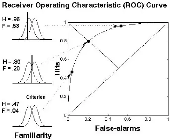

![Figure 2.4. Construction of ROC curve from frequency data.Receiver Operating Characteristic (ROC) curves can be constructed from participants’ data byplotting hits [P(“old”|old)] against false alarms [P(“old”|new)] across different confidence levels.Probab](https://thumb-us.123doks.com/thumbv2/123dok_us/9746114.475628/86.595.108.466.70.531/construction-operating-characteristic-constructed-participants-byplotting-different-confidence.webp)