Testing time invariance of process parameters in serious games : measured and applied in the application game Leo’s Pad

(1)

1

Bachelor thesis Psychology

Testing time invariance of process

parameters in serious games

Measured and applied in the application game Leo’s Pad

Name

Cornelieke van Steenbeek

Student ID

s1369644

Faculty

Faculty of Behavioural, Management

and Social Sciences

Department

Department of Research

Methodology, Measurement and Data

Analysis

Supervisor

prof. dr. ir. J.P. Fox

(2)

2

children are joining young Leonardo da Vinci on adventures through which they will learn concepts like problem solving, creative thinking, social emotional awareness and other. The purpose of the application is to learn children about the world through games. This concept is part of another concept called serious gaming: gaming for a primary purpose other than pure entertainment.

Giving feedback has an important role in serious gaming. Burgers, Eden, van Engelenburg and Buningh (2015) point out that this is important when it comes to staying motivated to play a game. Players that receive negative feedback feel less competent and are more willing to play the serious game to improve their performance. Players that receive positive feedback felt more competent and autonomous which made them desire to play a higher level in the game which may lead to long-term play. An important question that comes to mind is how to integrate this feedback in serious games like Leo’s Pad and how to detect whether or not players need feedback and in what form.

The children that are playing Leo’s Pad are getting feedback about whether they are giving the right or wrong answer. And there lies an opportunity to get some insight in their learning process for parents and teachers. However, it is not yet possible to give direct feedback about their learning process while they are playing the game. One way to do this is to personalize the game as much as possible (Kickmeier-Rust, Augustin & Albert, 2011). Gamers who get immediate feedback by intelligent and adaptive tutoring, get more involved and motivated to play the game. For example, when a child completes a level far more quickly than he/she

normally does or than his/her peers do, a different type of feedback should be given than when a child is much slower.

[image:3.612.151.461.507.699.2]

Firstly, it was necessary to have a look at the game itself. This thesis will focus on the first part of the game, which is available for free in the appstore for Apple users (iPhone and iPad). In this part, gamers have to click on the right shapes in a room with different objects as shown in Figure 1 (Kidaptive, n.d.).

(4)

4

How long it takes to find the object (response time) is the most important data observation that will be used in this thesis. Höhle (2010) points out how change point detection can help to obtain information about the time sensitivity of the model describing the data. It can be useful to see if parameters of the different items/assignments of an underlying statistical model are invariant over time. Parameters of game levels are often assumed to be time invariant. Scores, according to the statistical model of a gamer (furthermore referred to as items), can be used to give reliable feedback such as information about the performance. When scores are used from a model with time-variant parameters, the time-specific model parameters are needed each time when feedback is given.

Therefore, it is important to test the invariance assumption of the parameters of the statistical model describing the data. This is done to find out if the mean parameter representing the item’s difficulty and the variance parameter representing the variability in response time given the item’s difficulty are consistent over time and are not sensitive to time-correlated variables like knowledge or impact of technology. This leads to the research question: how can variations over time in item characteristics of a statistical model describing the data be

identified? The developed tests will be applied to data of the learning game Leo’s Pad to test the time-invariant properties of the model describing the game’s items with respect to the response times. The idea is that a user can be flagged for performing significantly different on an item with respect to time, followed by a consequence yet to be devised. The gamer (in this case, the child) will then have to perform more seriously and will give the parents insight in how their child performs compared to a certain average (for example the average performance of other children of the same age). The game Leo’s Pad, and games in general, usually need to process a lot of data at once. To find a model fitting to this type of data selection it should be taken into account that it is not desirable to come up with a model that has to make a lot of calculations before it can be stated whether or not the model is fitting to the new data. It should therefore be kept in mind that this thesis will focus on finding a model for which it is only necessary to put in new data, which will result in a fitting or non-fitting model as the outcome (thus, without having to make a lot of calculations in advance).

Data description

The statistical model describing the data which is used to answer the research question is a data sample of the game ‘Leo’s Pad’. It is collected from 2013-03-20 to 2014-01-23 and contains several variables. Important variables for this thesis are ‘timestamp’, ‘item’ and ‘response time’. Those variables will now be explained individually.

Timestamp

Timestamp is the date and time of the registration of the data. It is given in seconds. This data is important for the research question of this thesis; to know if the parameters of response times are invariant over time, it is necessary to know at what time the data has been measured. To work with the variable timestamp, it is transformed to a new variable where the first registered response observation (2013-03-20) is regarded as the zero time point. The function POSIXlt in the statistical software R is used to construct the new variable. Subsequently, for each

observation the difference in time is computed with the first observation. This new variable will be used to identify change of parameters of the model for response times.

Item

(5)

5

is a factor variable which contains 127 different levels. So, the game contains a total of 127 items.

Response time

The response time is the time gamers need to finish an item. It is the time a child uses from the moment it is given the item until the moment the child clicks or taps on an object (regardless of whether the item is done correctly). The response time is registered in thousandths of a second accuracy. The response time data is distorted because of some extreme outliers. The maximum measured time is 28,392.570 seconds while the median is 4.660. The cause of those extremes could be an error in the game’s system or a gamer who lost its concentration and stopped playing the game without closing it. Because the cause is unknown, it is important to be careful with correcting the data. The maximum could be cut off at a time that is long enough to do the

assignment (like 50 seconds should be long enough). However, this decision will maybe exclude non-concentrated gamers, which are part of the target group of this study. Therefore, the

maximum response time is cut off at 200 seconds, which allows some extreme scores to be flagged, but also brings the mean of the response times closer to its median, as shown in Figure 2. It also doesn’t exclude much of the observations. At first there were 228,576 observations, after correction there were 228,050 left (an exclusion of less than 0,3% of all observations). The response time is considered to be an outcome variable of the statistical model. Extreme outliers will seriously influence the estimates of the model parameters. To avoid the influence of such unlikely observations, they have been discarded in the analysis.

[image:5.612.335.538.268.385.2]

The response times are transformed to a lognormal distribution to get the most complete and relevant information. By doing this, there is no limitation at 0 anymore because negative values are also a possibility (Figure 3). Another positive effect is that the logarithm of the response times are correcting outliers of the data which makes it more normally distributed and less positive skew (Figure 4). Figure 5 supports this by showing the results in Q-Qplots. The x-axes

Figure 2 Responsetime parameters comparison before and after assigning a maximum of 200 seconds

[image:5.612.49.567.501.726.2]

(6)

6

show the quantiles that are theoretically expected for the data when a normal distribution is assumed. The y-axes show what the quantiles of the sample group are. As shown, the ordered logarithm of response times show a better resemblance with the theoretical quantiles of the normal distribution, and, therefore, the normal distribution better applies to the log response times than the response times.

A statistical model is used to describe the logarithm of the response times (RTip, the indices

[image:6.612.49.568.100.373.2]

refer to (i)tem and (p)erson). The response time is distributed with an average time that is needed

Figure 4 Comparison of normal distribution of original responsetime (left) and logresponsetime (right) of item 1

[image:6.612.50.569.157.585.2]

(7)

7

to complete an item. This parameter is referred to as time intensity (λi). The parameter speed is

the work speed of a person when he/she makes an assignment (speedp). In addition, there is a

certain scattering (error: eip) around λ. When time intensity is reduced by work speed and the

error is added it will give the response times as formulated in this formula:

𝑅𝑇𝑖𝑝= 𝜆𝑖 − 𝑠𝑝𝑒𝑒𝑑𝑝+ 𝑒𝑖𝑝

In this model, eip is normally distributed with mean = 0 and σ1 is the variation in the working

speed of a person and σ2 can be explained as random error variance (noise) that occurs because

of interfering external factors. Because the focus of this research is on the parameters of a statistical model describing the items, all parameters that say something about individuals (a person) should be left out of the model distribution. This results in the following model in which eip is distributed with N(0, σ1+σ2):

𝑅𝑇_𝑖𝑝= 𝜆_𝑖+ 𝑒_𝑖𝑝

The parameters of this model that can be used for testing are time intensity (λ) and the variance of e (σ= σ1+σ2).

Statistical process control

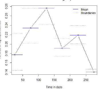
Sometimes a certain process has to be monitored and controlled to give feedback to a user. When statistical analyses are involved, this phenomenon is called statistical process control. A lot of processes can be expressed in quantitative measurements like time, distance, height and so forth. When it is desired to control a process variable, it is a common practice to control both the mean and the variance of the variable. When a data sample is taken from a population, the mean and the variance of the variable of the population (µ and σ) can be estimated by using the sample mean and the sample variance of the sample group. With the sample data, the range of the mean of the population can be estimated with an upper boundary and a lower boundary (the same goes for the variance). For example, for a sample of 100 observations, the mean response time of the population of all gamers will be estimated between 1 and 8 seconds (the lower and upper boundary of a confidence interval of time intensity). This statement can be made with different reliability percentages. This goes with the rule that when you want to be less sure (like 90%), the range will be smaller than when you want to be more sure (like 99%) that the range contains the mean of the population.

(8)

[image:8.612.115.477.74.378.2]

8

Figure 6 Controlchart for the mean of the logresponsetime of item 1 in timeframes of 50 days

[image:8.612.129.471.435.746.2]

(9)

9

With all this information, three types of models can be described. The first type of model that can be used, is a model that tests the two parameters separately. This results in a model whereby new data of new timeframes will be tested to be in or out of control with the parameters of the first timeframe. λ2, λ3, λ4 (the indices refer to the timeframes) and so on will be tested to be

in control with λ1. And σ2, σ3, σ4 and so on will be tested to be in control with σ1. The second

model can combine these two parameters and see if (λ2, σ2), (λ3, σ3), (λ4, σ4) is in control with the

model’s parameters (λ1, σ1). The last model option consists of λ1 andσ1 and the upper and lower

boundary these parameters. When new data comes in, it is only important to see if the new data is in control between these boundaries. The next paragraph will describe ways to design and test the different types of models.

Testing the parameters of the log response time using different timeframes

To test whether the parameters of the log response time are invariant over time, it is necessary to test the parameters with the proper statistical test. Here, time intensity (λ) will be tested on time invariance. Then, the variance will be tested on time invariance. Subsequently, time intensity and variance will be tested in one comprehensive test together. In all tests 3 items will be tested: item 1, 3 and 7. The items are mainly picked randomly, the only condition is that the item has enough observations.

Testing Lambda with an independent 2-group t-test

A fitting statistical test should be found to test the parameter time intensity (λ) on time

invariance. One of the statistical tests that can be used is the "independent samples" t-test. It’s formula is written as follows:

t = 𝜆1− λ2

√s12

n₁ + s2

2

n₂

This test will compare the time intensity of two timeframes with each other to see how much they are correlated. The outcome will consist a p-value that will indicate whether or not the samples significantly differ (p<0.05 refers to a significant difference).

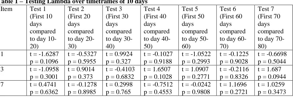
[image:9.612.77.569.535.701.2]

To see how much of a difference the width of a timeframe makes, there are test results shown for three different timeframe sizes: 10 days, 50 days and 80 days shown in Table 1, 2 and 3, respectively.

Table 1 – Testing Lambda over timeframes of 10 days

Item Test 1 (First 10 days compared to day 10-20)

Test 2 (First 20 days compared to day 20-30)

1 t = -1.6287

p = 0.1096

t = -0.5327 p = 0.5955

t = 0.9924 p = 0.327

t = -0.1027 p = 0.9188

t = -1.0522 p = 0.2993

t = -0.1225 p = 0.9028

t = -0.6698 p = 0.5044

3 t = -1.0958

p = 0.3001

t = 0.9014 p = 0.373

t = -0.4103 p = 0.6832

t = 1.6507 p = 0.1028

t = 1.0907 p = 0.2771

t = -0.2116 p = 0.8326

t = 1.687 p = 0.0944

7 t = 0.4741

p = 0.6362

t = -0.1278 p = 0.8985

t = 0.2998 p = 0.765

t = -0.7512 p = 0.4553

t = -0.0242 p = 0.9808

t = 1.1696 p = 0.2721

(10)

[image:10.612.74.578.96.229.2]

10 Table 2 - Testing Lambda over timeframes of 50 days

Item Test 1 (First 50 days compared to day 50-100)

Test 5 (First 250 days compared to day 250 and later)

1 t = -1.8132

p = 0.0706

t = -2.3271 p = 0.02021

t = -1.0321 p = 0.3022

t = -1.2874 p = 0.1981

t = 1.0298 p = 0.3031

3 t = -0.2069

p = 0.8364

t = -1.7678 p = 0.07724

t = -0.0447 p = 0.9644

t = 1.6251 p = 0.1042

t = 0.7154 p = 0.4744

7 t = 0.7294

p = 0.4663

t = 0.7739 p = 0.4436

t = 1.3293 p = 0.1976

t = -0.8256 p = 0.4464

[image:10.612.73.576.260.385.2]

t = 0.1447 p = 0.8939

Table 3 - Testing Lambda over timeframes of 80 days

Item Test 1 (First 80 days

compared to day 80-160)

Test 5 (First 240 days compared to day 240 and later)

1 t = -2.7944

p = 0.005361

t = -1.0063 p = 0.3144

t = 0.6878 p = 0.4916

3 t = -3.151

p = 0.001755

t = 0.7715 p = 0.4405

t = 1.168 p = 0.2428

7 t = 1.0078

p = 0.3143

t = 0.934 p = 0.3623

t = -0.9059 p = 0.4063

Testing variance with the chi-square test

For the variance of the log response time another test should be used. A chi-square test is a good choice to see if the variances of the log response times are significantly different from each other in the several timeframes,. The formula for the chi-square test is:

2 ₌(n − 1)s12

s₂2

The outcomes given in Table 4 for item 1, 3 and 5 are p-values following from the chi-square test. This outcome indicates how much the variance of a timeframe deviates from the variance of the first timeframe. When 2is close to 1, then s2 (estimated sample variance following from data

of a new timeframe) is smaller than s1 (sample variance computed in first timeframe). And when

it is close to 0, s2 is greater than s1. When this difference is significant (more than 0.95 or less

[image:10.612.62.580.608.679.2]

than 0.05) the next test with the next timeframe will be carried out with the data of the last timeframe (s2 as new s1).

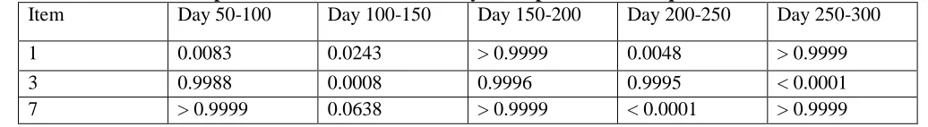
Table 4 - Variance comparison in timeframes of 50 days with p-value of chi-square test

Item Day 50-100 Day 100-150 Day 150-200 Day 200-250 Day 250-300

1 0.0083 0.0243 > 0.9999 0.0048 > 0.9999

3 0.9988 0.0008 0.9996 0.9995 < 0.0001

(11)

11

Testing Lambda and the variance with the likelihood-ratio test

Now it is known how the different Lambda’s compare to one another and how the different variances compare to one another. But this is actually not completely what is needed to know. It would be more convenient to test Lambda and the variance with the same test. The likelihood-ratio test can be used for this purpose. With a likelihood likelihood-ratio test, the goodness of fit of two models can be compared. The formula of this test is:

𝐿𝑅 = 𝐿(𝛺0) 𝐿(𝛺₁)

In this formula, the largest value of the likelihood of H0 is called the likelihood function L(Ωo).

The largest value of the likelihood of H1 is called the likelihood function L(Ω1). When L(Ω1) is

much larger than L(Ω0), hypothesis H0 should be rejected.

To test if the variance of different timeframes of a specific item do significantly differ from each other, the likelihood ratio of the variance of timeframe 1 and the data of timeframe 2 are compared. In order to do this, this test compares the old parameters of timeframe 1 (Ωo) with

the best fitting parameters to timeframe 2 (Ω1). This will always give a negative test outcome,

steering to the parameters of Ω1. When Ω1 is close to Ωo,the test outcome will be close to 0,

because the data has a lognormal distribution. This is in favor of Ωo when the p-value of the

likelihood-ratio test is 0.05 or higher. When this is the case, the parameters of the new data are considered fitting to the parameters of the model and are not rejected. When the test value significantly deflects from 0 (the p-value of the likelihood-ratio test is less than 0,05), the new data is considered out of control. In this case the new data of timeframe 2 will be used to

[image:11.612.79.573.433.560.2]

calculate the parameters for the next null hypothesis, to which the data of the next timeframe (3) shall be tested. Table 5 shows the results of this testing method for item 1, 3 and 5.

Table 5 – Likelihood ratio test of the variance comparing old timeframe parameters with best fitting parameters of the data of a later timeframe

Item Test 1 (input: data day 50-100)

Test 2 (input: data day 100-150)

Test 5 (input: data day 250 and later)

1 LR = -6.8514

p = 0.0002

LR = -2.7722 p = 0.0185

LR = -22.9186 p < 0.0001

LR = -4.7849 p = 0.0020

LR = -179.9553 p < 0.0001

3 LR = -32.3156

p < 0.0001

LR = -8.5748 p < 0.0001

LR = -8.0784 p < 0.0001

LR = -7.0790 p < 0.0001

LR = -65.7770 p < 0.0001

7 LR = -3.5514

p = 0.0077

LR = -0.3400 p = 0.4096

LR = -4.8792 p = 0.0018

LR = -42.8224 p < 0.0001

LR = -2.132492 p = 0.0389

Another way of using the likelihood-ratio test is by using the boundaries of a confidence interval of a parameter. In this case, in examining the variance of the response time, Ωo is still the

variance of the first timeframe. Ω1 however is now the upper or lower boundary of the 95%

confidence interval of the estimated variance of the first timeframe. When the data of a new timeframe is tested and the LR value is positive, the process is in control since there is no change detected in the sample variance. When the LR value is significantly negative, the process is out of control and a significant change in the variance parameter is detected. This gives information about the direction the new data is going and how steep this shift is. When the outcome of LR has no significant p-value, the model’s parameters can still be used for testing the other

(12)

12

[image:12.612.75.593.142.275.2]

be taken into account (depending on the purpose of testing). Table 6 shows the test results of this way of testing. This time, item 106 is tested.

Table 6 – Likelihood-ratio test comparing timeframes with the variance of the first timeframe and its boundaries

All data is compared to the parameters of the first timeframe (day 0-50)

Test 1 (Data day 50-100)

𝐿(𝛺_{𝑉𝑎𝑟𝑖𝑎𝑛𝑐𝑒}) 𝐿(𝛺_{𝑈𝑝𝑝𝑒𝑟 𝐵𝑜𝑢𝑛𝑑𝑎𝑟𝑦})

LR = 19.3864 p < 0.0001

LR = 29.8663 p < 0.0001

LR = 46.9374 p < 0.0001

LR = 94.5212 p < 0.0001

LR = 199.2003 p < 0.0001

𝐿(𝛺_{𝑉𝑎𝑟𝑖𝑎𝑛𝑐𝑒}) 𝐿(𝛺_{𝐿𝑜𝑤𝑒𝑟 𝐵𝑜𝑢𝑛𝑑𝑎𝑟𝑦})

LR = 6.1800 p = 0.0004

LR = 7.43444 p = 0.0001

LR = 10.0074 p < 0.0001

LR = -12.8328 p < 0.0001

LR = 5.9049 p = 0.0006

With this outcome it can be said whether or not the process is in or out of control, in this case it is clearly in control. For a comparison, Figure 8 shows a graph with the variances of all

timeframes and the boundaries of the variance of the first timeframe. The likelihood ratio-test gives this information already without having to calculate all the parameters of the different timeframes.

Conclusion

This research started with the question: how can variations over time in item characteristics of a statistical model describing the data be identified? A few conclusions can be drawn based on the results of the three tests for the response time models for the application game Leo’s Pad.

The two parameters that are used to describe the response times are time intensity (λ) and the variance of the response times (σ). Time intensity has been tested on time invariance using an

[image:12.612.80.517.341.568.2]

(13)

13

independent sample t-test. For this purpose, the response time is divided into different

timeframes of 10, 50 and 80 days. The results of these tests show only a few significant results, even in the table with timeframes of 80 days. Dependent on these results it can be stated that the mean of the variable response times is fairly consistent over time. In this case and only with this dataset, λ of the response times of the items is invariant over time. This means that this test is useful for testing the time invariance of the response times of this application game.

The error variance parameter of the model for the response times is tested with the chi-square test. This test gives information about which variance of two different timeframes is bigger and whether this difference is significant. The test results show almost exclusively significant results, which means that the error variance of the analyzed response time changed over time data. The chi-square test is therefore also useful to test the time invariance of the response times of the application game.

The parameters are tested with two different likelihood-ratio tests. The first test used the best fitting parameters of the new data as the alternative hypothesis. The null hypothesis is calculated with the parameters of the response time model of the first timeframe. The likelihood-ratio test had, because of testing the same items, the same outcome as the chi-square test but also includes the parameter time intensity. The second likelihood-ratio test, provided even more information. This test shows the results of a different item. Even though the results show almost exclusively significant results in favor of the null hypothesis, the outcome still tells something about the direction of evidence of the new data. The results are a quantitative visualization of how much the data deviates from the variance of the first timeframe and if it stays and is expected to stay within the boundaries of the 95% confidence interval of this variance. This second likelihood-ratio test does this without having to calculate all the parameters for every new timeframe. The second likelihood-ratio model therefore seems the most efficient way to identify variations in item characteristics over time.

Discussion

The likelihood-ratio test using the lower and upper boundaries of the variance as alternative hypothesis is a very efficient test to use in process control. The test only requires the parameters of the first timeframe. After that, new data is used see if the model fits to the new data. It is just a matter of sampling new data and see if the model still fits to it. When there is a shifting to one of the boundaries it can be noted in an early stadium and dealt with. The greatest benefit of this method is that is doesn’t require a calculation of the parameters for every new timeframe.

Another benefit of this test is that it can be used for any quantitative parameter of any variable of any process control data. This research could have been more generalized when it include a likelihood-ratio examination of λ instead of only examining σ. And this test could have been used for far more other purposes. Setting up a similar test situation for λ with the

(14)

14 References

Burgers, C., Eden, A., Van Engelenburg, M.D., Buningh, S. (2015). How feedback boosts motivation and play in a brain-training game. Computers in Human Behavior, 48, 94-103. doi: 10.1016/j.chb.2015.01.038

Höhle, M. (2010). Online Change-Point Detection in Categorical Time Series. Statistical Modelling and Regression Structures, 377-397. doi: 10.1007/978-3-7908-2413-1 20 Kickmeier-Rust, M.D., Augustin, T. & Albert, D. (2011). Personalized storytelling for

educational computer games. Lecture Notes in Computer Science,6944, 13-22. doi: 10.1007/978-3-642-23834-5_2

(15)

15 Appendix

R-code used designing this research

data <- #data input from Leo’s Pad

N <- nrow(data)

nll <- tapply(rep(1,N),data$item,sum)

data1 <- data[data$item == 106,]

N <- nrow(data1)

out <- lm(responsetime ~ 1+outcome, data=data1) summary(out)

set1 <- which(data1$responsetime > 200)

set <- which(data1$responsetime < 200 & data1$responsetime > 0) data11 <- data1[set,]

N <- nrow(data11)

out <- lm(responsetime ~ 1 + outcome, data=data11)

data11$timediff <- difftime(data11$time,min(as.POSIXlt(data11$timestamp)),unit="days") data11$logresponsetime <- log(data11$responsetime)

oo <- order(data11$timediff)

data11o <- data11[oo,] #new data frame ordered by timediff

N=10000

testdata <- rnorm(N, (mean(data11o$responsetime)), (var(data11o$responsetime)))

set1 <- which(data11o$timediff <= 50)

set2 <- which(data11o$timediff > 50 & data11o$timediff <= 100) set3 <- which(data11o$timediff > 100 & data11o$timediff <= 150) set4 <- which(data11o$timediff > 150 & data11o$timediff <= 200) set5 <- which(data11o$timediff > 200 & data11o$timediff <= 250) set6 <- which(data11o$timediff > 250)

RT1 <- data11o$logresponsetime[set1] RT2 <- data11o$logresponsetime[set2] RT3 <- data11o$logresponsetime[set3] RT4 <- data11o$logresponsetime[set4] RT5 <- data11o$logresponsetime[set5] RT6 <- data11o$logresponsetime[set6]

(16)

16

t.test(RT3,RT4) t.test(RT4,RT5) t.test(RT5,RT6)

N=sum(complete.cases(data11o$logresponsetime[set2])) sigma20 <- var(RT4)

varstat <- (N-1)*var(RT2)/sigma20 pchisq(varstat,df=N-1)

TestSigma <- function(RT,sigma,N){

RT <- matrix(RT,nrow=N) if(ncol(RT) > 1){

sigmahat <- apply(RT,2,var)

varstat <- (N-1)*apply(RT,2,var)/sigma

LRatio <- (N/2)*(1 + log(sigmahat/sigma) - (sigmahat/sigma)) }else{

sigmahat <- var(RT)

varstat <- (N-1)*var(RT)/sigma

LRatio <- (N/2)*(1 + log(sigmahat/sigma) - (sigmahat/sigma)) }

pvaluec <- pchisq(varstat,df=N-1) # H1 versus H0 pvalueLR <- 1-pchisq(-2*LRatio,df=1) # H1 versus H0

LowUpp <- c(qchisq(.025,df=N-1),qchisq(.975,df=N-1))

return(list(varstat=varstat,pvaluec=pvaluec,pvalueLR=pvalueLR,LowUpp=LowUpp,LRatio=LR atio))

}

TestSigma(RT=RT6,sigma=var(RT5),N=sum(complete.cases(data11o$logresponsetime[set6])))

par3 <- '0.95' par2 <- var(RT1)

par1 <- sum(complete.cases(data11o$logresponsetime[set1])) par1<-as.numeric(par1)

par2<-as.numeric(par2) par3<-as.numeric(par3) df <- par1 - 1

halfalpha <- (1 - par3) / 2

right <- par2 * df / qchisq(halfalpha,df) left <- par2 * df / qchisq(1-halfalpha,df)

(17)

17

LRatio <- sum(dnorm(RT,mean=mean(RT),sd=sqrt(sigma),log=T)) - sum(dnorm(RT,mean=mean(RT),sd=sqrt(sigmahat),log=T))

pvalueLR <- 1-pchisq(abs(-2*LRatio),df=1) # H1 versus H0

return(list(pvalueLR=pvalueLR,LRatio=LRatio)) }

TestSigmaLR(RT=RT6,sigma=var(RT1),sigmahat=right,N=sum(complete.cases(data11o$logres ponsetime[set6])))

TestSigmaLR(RT=RT6,sigma=var(RT1),sigmahat=left,N=sum(complete.cases(data11o$logresp onsetime[set6])))

x <- data11o$timediffgraph

y <- data11o$logresponsetimegraph

plot(x, y, xlim = c(0,300), ylim = c(0.21, 0.32), type="b", xlab="Time in days", ylab="Variance of logresponsetimes", main="Controlchart for variance of the logresponsetime of item 6")

segments(x=0, y=(var(RT1)), x1=300, y1=(var(RT1)),col=4,lty=1) par3 <- '0.95'

par2 <- var(RT1)

par1 <- sum(complete.cases(data11o$logresponsetimegraph[set1])) par1<-as.numeric(par1)

segments(x=0,y=left,x1=300,y1=left,col=4,lty=3)

x <- data11o$responsetime

h<-hist(x, breaks=15, col="cadetblue", xlab="Responsetime in seconds", main="Histogram of original responsetime with Normal Curve")

xfit<-seq(min(x),max(x),length=100) yfit<-dnorm(xfit,mean=mean(x),sd=sd(x)) yfit <- yfit*diff(h$mids[1:2])*length(x) lines(xfit, yfit, col="darkred", lwd=2)

x <- data11o$logresponsetime

h<-hist(x, breaks=15, col="cadetblue", xlab="Logresponsetime", main="Histogram of logresponsetime with Normal Curve")

xfit<-seq(min(x),max(x),length=100) yfit<-dnorm(xfit,mean=mean(x),sd=sd(x)) yfit <- yfit*diff(h$mids[1:2])*length(x) lines(xfit, yfit, col="darkred", lwd=2)

(18)

18

plot(x,y,type="l", xlab="Time in days (day 0 = first day of data sampling)", ylab="Responsetime in seconds")

y <- data11o$logresponsetime

plot(x,y,type="l", xlab="Time in days (day 0 = first day of data sampling)", ylab="Logresponsetime")

#qplots

qqnorm(data11o$responsetime, ylab="Quantiles original responsetime") qqnorm(data11o$logresponsetime, ylab="Quantiles logresponsetime")

data11o$timediffgraph <- data11o$timediff

data11o$timediffgraph[data11o$timediffgraph <= 50] <- 25

data11o$timediffgraph[data11o$timediffgraph > 50 & data11o$timediffgraph <= 100] <- 75 data11o$timediffgraph[data11o$timediffgraph > 100 & data11o$timediffgraph <= 150] <- 125 data11o$timediffgraph[data11o$timediffgraph > 150 & data11o$timediffgraph <= 200] <- 175 data11o$timediffgraph[data11o$timediffgraph > 200 & data11o$timediffgraph <= 250] <- 225 data11o$timediffgraph[data11o$timediffgraph > 250] <- 275

data11o$logresponsetimegraph <- data11o$logresponsetime data11o$logresponsetimegraph[set1] <- mean(RT1)

data11o$logresponsetimegraph[set2] <- mean(RT2) data11o$logresponsetimegraph[set3] <- mean(RT3) data11o$logresponsetimegraph[set4] <- mean(RT4) data11o$logresponsetimegraph[set5] <- mean(RT5) data11o$logresponsetimegraph[set6] <- mean(RT6)

#Graph mean:

plot(x, y, type="b", xlab="Time in days", ylab="Mean of logresponsetimes", main="Controlchart for mean of the logresponsetime of item 1")

segments(x=0, y=(mean(data11o$logresponsetime[set1])), x1=50, y1=(mean(data11o$logresponsetime[set1])),col=4,lty=1)

error <-

qt(0.975,df=length(data11o$logresponsetime[set1])-1)*sd(data11o$logresponsetime[set1])/sqrt(length(data11o$logresponsetime[set1])) left <- mean(data11o$logresponsetime[set1])-error

right <- mean(data11o$logresponsetime[set1])+error segments(x=0,y=left,x1=50,y1=left,col=4,lty=3) segments(x=0,y=right,x1=50,y1=right,col=4,lty=3)

segments(x=50, y=(mean(data11o$logresponsetime[set2])), x1=300, y1=(mean(data11o$logresponsetime[set2])),col=4,lty=1)

error <-

qt(0.975,df=length(data11o$logresponsetime[set2])-1)*sd(data11o$logresponsetime[set2])/sqrt(length(data11o$logresponsetime[set2])) left <- mean(data11o$logresponsetime[set2])-error

right <- mean(data11o$logresponsetime[set2])+error segments(x=50,y=left,x1=300,y1=left,col=4,lty=3) segments(x=50,y=right,x1=300,y1=right,col=4,lty=3)

legend("bottomright",col=4,lty=c(1,3), lwd=1,legend=c("Mean", "Boundaries"), bty="n")

(19)

19

data11o$logresponsetimegraph[set1] <- var(RT1) data11o$logresponsetimegraph[set2] <- var(RT2) data11o$logresponsetimegraph[set3] <- var(RT3) data11o$logresponsetimegraph[set4] <- var(RT4) data11o$logresponsetimegraph[set5] <- var(RT5) data11o$logresponsetimegraph[set6] <- var(RT6)

#Graph variance:

plot(x, y, type="b", xlab="Time in days", ylab="Variance of logresponsetimes", main="Controlchart for variance of the logresponsetime of item 1")

par2 <- var(RT1)

segments(x=0,y=left,x1=50,y1=left,col=4,lty=3) segments(x=0,y=right,x1=50,y1=right,col=4,lty=3)

par2 <- var(RT2)

segments(x=100, y=(var(RT3)), x1=150, y1=(var(RT3)),col=4,lty=1) rrpar3 <- '0.95'

par2 <- var(RT3)

(20)

20

left <- par2 * df / qchisq(1-halfalpha,df)

par2 <- var(RT4)

par2 <- var(RT5)